Energy-Feedback Load Simulation Algorithm Based on Fuzzy Control

Abstract

In order to solve the problem that the traditional Proportional Integral (PI) controller cannot take into account both response speed and input current overshoot and cannot adapt to complex working conditions, an energy-feedback DC load simulation control algorithm based on fuzzy control was proposed. By adding a fuzzy adaptive PI setting to the traditional load simulation control algorithm, the dynamic response performance of the system and the accuracy of load simulation were improved. A small-signal model of a load analog boost circuit was established based on the state average method. Based on the phase margin, the PI parameter setting of series correction was completed, and the corresponding fuzzy control rules were formulated to identify the response state. Simulation results show that the regulation time of constant current load simulation based on a fuzzy control strategy is shortened by 75.2%, the steady-state error is reduced by 60%, and the overshoot is reduced from 28.3% to 7.47%. The prototype test results show that the maximum relative error of input current load simulation is only 4.50%, and the system response speed can meet the requirements of variable load simulation. The results show that the load simulation control algorithm based on fuzzy control has the characteristics of high precision and excellent dynamic characteristics.

1. Introduction

Uninterruptible power supply, power battery, and charging pile, such as power equipment in the process of manufacturing, require a series of strict product testing. Load can be traditional and electronic. The energy consumption in the process of load simulation, the output energy by measuring equipment on the load resistance, and power components such as heat dissipation assist the cooling device. The energy-fed electronic load does not have energy dissipation devices, and the test energy is conveyed to the public grid or the input end of the tested equipment through the switching circuit, thus forming an energy loop, which not only completes the load simulation function but also realizes the energy recovery.

The front stage of the energy-fed AC electronic load is the load simulation unit, which not only realizes the high-precision load simulation but also undertakes the function of rectifier and voltage boost. The PI parameters of a traditional load simulation PI control algorithm are fixed values, which cannot adapt to complex load simulation conditions [1]. It is easy to cause system overshoot and steady-state errors, and there are certain limitations on the stability and response speed of the system. Therefore, the accuracy of load simulation and steady-state precision of overload are a great test. At the same time, when the load analog boost circuit only adopts the traditional PI control, it cannot give good consideration to the problem of response speed and current overshoot. In order to obtain faster dynamic response, the input current overshoot will be larger [2]. In light of this, the over-current protection of the triggered system will lead to the restart of the energy-fed DC electronic load, which will lead to the damage of components and increase the cost of operation and maintenance. Therefore, an efficient and high-precision control algorithm is very important for simulating load cells.

The load simulation algorithm in Reference [3] adopts voltage single-closed-loop PI control, compares input voltage with the reference voltage, passes through a PI controller, and finally outputs the control signal used to control the phase-shifted full-bridge load analog circuit. Reference [4] adopted an integrated automatic control single-cycle controller chip and reconfigurable field-programmable analog array. With its simple interface structure, it does not need to adopt DSP to design a control algorithm, which saves the cost of research and development. In Reference [5], the former load analog circuit adopted the repetitive control algorithm based on the internal model principle and improved the robustness of the control system by introducing historical deviation information. The steady-state performance of the system was good. Recent works [6,7] used the recharging structure of the converter circuit; that is, using the proposed resonant load with a wide variety of speeds and continuous loading function, the feasibility of the tested battery was verified, and the energy recycling was realized in the test process.

Aiming at the problem that PI control depends on the system model, a load simulation control strategy was proposed in Reference [8], which combines single-cycle control with PI control. The control algorithm switcher can switch between PI control and single-cycle control according to the given quantity and feedback quantity. Therefore, it has the advantages of the fast dynamic response of single-cycle control and high steady-state precision of PI control. In References [9,10], a load analog control algorithm of the digital outer loop and analog inner loop was proposed. The given current reference value was obtained by the digital outer loop and then converted to the analog inner loop. The analog inner loop is a special analog control chip for the power circuit. The algorithm has a fast response speed and can realize cycle-by-cycle current control, but there is a temperature drift problem, which affects the control accuracy.

In addition to PI control, other basic control algorithms are often applied to the power feed grid control, such as deadbeat control, PR (Proportional Resonance) control, single period control, and so on. According to the circuit equation, the duty-cycle mathematical model is established for the beat-free control. By sampling the circuit parameters of the current cycle, the duty cycle of the full-bridge driver in the next cycle is calculated. It belongs to precise control, and the principle is simple and easy to understand and easy to design [11]. PR controller can achieve high gain without static error tracking near the resonant point and can greatly suppress signals of other frequencies. However, its bandwidth depends on the stability of power grid frequency, and thus it is not suitable for the power feed [12].

None of the above control algorithms can achieve fast and efficient control. Aiming at the key technical problems such as transient performance, steady-state accuracy, power feedback quality, and overall efficiency of energy-fed DC electronic load, this paper focuses on a kind of high-efficiency energy-fed DC electronic load with medium and high voltage input and its control strategy. In this paper, the high-efficiency regenerative DC electronic load adopts the “boost+ full bridge” as the power circuit topology. Aiming at the transient performance and steady-state accuracy of the energy-regenerative DC electronic load, an input-current-tracking algorithm based on fuzzy control is proposed. In this paper, the control strategy of high-efficiency feed-DC electronic load is studied systematically, and the correctness of the theoretical analysis and feasibility of the scheme are verified by relevant simulation experiments.

2. Load Simulation Small-Signal Modeling

According to the test requirements and power feature of the DC power supply, only resistive loads are required during testing. Therefore, DC electronic load just has to simulate pure resistance load, not the capacitive load and inductive load. Moreover, only the three basic modes of constant power, constant current, and constant resistance are needed for load simulation [13], which can be respectively completed by making the DC electronic load’s input current I_IN, equivalent resistance R_L, and power output P_IN equal to the set value. The control objects of different load simulation modes are different and are not conducive to the subsequent control algorithm design and control loop compensation. Among them, the current control not only has fast dynamic response but can also realize the limitation of the peak current of each cycle. Therefore, the core idea of control object normalization is to convert the control of different load simulation modes into the tracking of input current I_IN. The normalized calculation formula of the control object is:

$$\{\begin{array}{l}{I}_{\mathrm{IN}\_\mathrm{Ref}}=\frac{P_{\mathrm{SET}}}{u_{\mathrm{IN}}}\left(\mathrm{C}\text{-}\mathrm{P}\mathrm{mode}\right)\\ I_{\mathrm{IN}\_\mathrm{Ref}}=\frac{u_{\mathrm{IN}}}{R_{\mathrm{SET}}}\left(\mathrm{C}\text{-}\mathrm{R}\mathrm{mode}\right)\\ I_{\mathrm{IN}\_\mathrm{Ref}}=I_{\mathrm{SET}}\left(\mathrm{C}\text{-}\mathrm{I}\mathrm{mode}\right)\end{array}$$

(1)

where I_{IN_REF} is the reference value of input-current-tracking instruction for high-efficiency feed-type DC electronic load, P_SET is the set power, R_SET is the set resistance, I_SET is the set current, and u_IN is the input voltage.

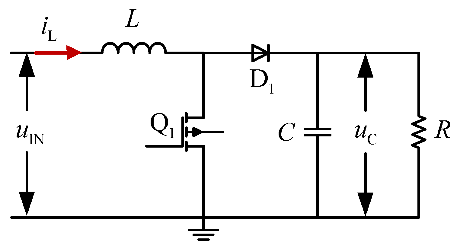
Load simulation boost circuit adopts closed-loop control; thus the dynamic model and transfer function of the boost circuit are needed to design the feedback loop so as to improve the steady-state precision and dynamic performance of the system. Since the load analog circuit contains boost switch tubes and diodes and other nonlinear devices, which are nonlinear systems [14,15], the state average method is adopted for modeling. Load simulation boost circuit diagram and component parameters are shown in Figure 1; i_L is the current through the inductor, u_IN is the input voltage, and u_C is the voltage at both ends of the capacitor.

It is assumed that the boost is in continuous on–off mode when working normally. The on–off voltage drop is ignored when the switch tube is on, which can be regarded as a short-circuit state. Similarly, it can be regarded as a cut-off state when the switch tube is turned off. In addition, the diode D1 conduction voltage drop is only 0.7 V, far less than boost input and output voltage, and thus can be ignored. According to the analysis in Section 2, the boost circuit has two operating modes, and when it operates in the on mode, the matrix equation describing the current circuit state is:

$$\left[\begin{array}{c}\frac{\mathrm{d}{i}_{\mathrm{L}}}{\mathrm{d}t}\\ \frac{\mathrm{d}{u}_{\mathrm{C}}}{\mathrm{d}t}\end{array}\right]=\left[\begin{array}{cc}0& 0\\ 0& \frac{-1}{RC}\end{array}\right]\left[\begin{array}{c}{i}_{\mathrm{L}}\\ u_{\mathrm{C}}\end{array}\right]+\left[\begin{array}{c}\frac{1}{L}\\ 0\end{array}\right]u_{\mathrm{IN}}$$

(2)

where t is the response time.

When the boost circuit operates in off mode, the matrix equation describing the current circuit state is:

$$\left[\begin{array}{c}\frac{\mathrm{d}{i}_{\mathrm{L}}}{\mathrm{d}t}\\ \frac{\mathrm{d}{u}_{\mathrm{C}}}{\mathrm{d}t}\end{array}\right]=\left[\begin{array}{cc}0& \frac{-1}{L}\\ \frac{1}{C}& \frac{-1}{RC}\end{array}\right]\left[\begin{array}{c}{i}_{\mathrm{L}}\\ u_{\mathrm{C}}\end{array}\right]+\left[\begin{array}{c}\frac{1}{L}\\ 0\end{array}\right]u_{\mathrm{IN}}$$

(3)

According to the concept of state-space average, the average switching period of the state variable is defined as:

$$<x(t){>}_{T_{\mathrm{S}}}=\frac{1}{T_S}{\displaystyle {\int }_t^{t+T_S}x(\tau )}\mathrm{d}\tau$$

(4)

where T_S is the average switching period, and τ is the response time.

Inductance current and capacitance voltage vary less in boost circuit operating modes, and their rate of change is approximately constant. Firstly, the values of the state variables at the end of the on mode and off mode are solved and then obtained by combining with Euler’s formula:

$$\left[\begin{array}{c}\frac{\mathrm{d}<i_{\mathrm{L}}{>}_{T_{\mathrm{S}}}}{\mathrm{d}t}\\ \frac{\mathrm{d}<u_{\mathrm{C}}{>}_{T_{\mathrm{S}}}}{\mathrm{d}t}\end{array}\right]=\left[\begin{array}{c}\frac{1}{L}\\ 0\end{array}\right]<u_{\mathrm{IN}}{>}_{T_{\mathrm{S}}}+\left[\begin{array}{cc}0& \frac{-d\prime }{L}\\ \frac{d\prime }{C}& \frac{-1}{RC}\end{array}\right]\left[\begin{array}{c}<i_{\mathrm{L}}{>}_{T_{\mathrm{S}}}\\ <u_{\mathrm{C}}{>}_{T_{\mathrm{S}}}\end{array}\right]$$

(5)

where $d\prime =1-d$,$d$ is boost driver duty cycle [16].

When the boost circuit operates stably, the average switching period of the state variable is constant, and thus Formula (5) can be solved to obtain:

$$\left[\begin{array}{c}{I}_{\mathrm{L}}\\ U_{\mathrm{C}}\end{array}\right]=\frac{-LC}{{\left(1-D\right)}^2}\left[\begin{array}{cc}\frac{-1}{RC}& \frac{1-D}{C}\\ \frac{-\left(1-D\right)}{L}& 0\end{array}\right]\left[\begin{array}{c}\frac{1}{L}\\ 0\end{array}\right]U_{\mathrm{IN}}$$

(6)

where $I_{\mathrm{L}}$, $U_{\mathrm{IN}}$, $U_{\mathrm{C}}$, $D$ are, respectively, the switching cycle average values of $i_{\mathrm{L}}$, $u_{\mathrm{IN}}$, $u_{\mathrm{C}}$, $d$ in the boost circuit at the static operating point.

Since the boost converter is a nonlinear system, its state-space average Equation (5) is a nonlinear equation, and thus it needs to be solved by the perturbation method. The core idea of the perturbation method is to make small perturbations of $i_{\mathrm{L}}$, $u_{\mathrm{IN}}$, $u_{\mathrm{C}}$, $d$ around the static operating point, which is the process of slightly changing the average switching period of each parameter after perturbation, compared with the average switching period of the state variable at the static operating point, as shown in Equation (7).

$$\{\begin{array}{l}<i_{\mathrm{L}}{>}_{T_{\mathrm{S}}}=I_{\mathrm{L}}+{\stackrel{⌢}{i}}_{\mathrm{L}}(t)\\ <u_{\mathrm{C}}{>}_{T_{\mathrm{S}}}=U_{\mathrm{C}}+{\stackrel{⌢}{u}}_{\mathrm{C}}(t)\\ <u_{\mathrm{IN}}{>}_{T_{\mathrm{S}}}=U_{\mathrm{IN}}+{\stackrel{⌢}{u}}_{\mathrm{IN}}(t)\\ d=D+\stackrel{⌢}{d}(t)\end{array}$$

(7)

After substituting Equation (7) into the nonlinear Equation (5), it is directly connected with Equation (6) and solved by ignoring the second-order AC term:

$$\left[\begin{array}{c}\frac{d{\stackrel{⌢}{i}}_{\mathrm{L}}(t)}{\mathrm{d}t}\\ \frac{d{\stackrel{⌢}{u}}_{\mathrm{C}}(t)}{\mathrm{d}t}\end{array}\right]=\left[\begin{array}{c}\frac{1}{L}\\ 0\end{array}\right]{\stackrel{⌢}{u}}_{\mathrm{IN}}(t)+\left[\begin{array}{c}\frac{U_{\mathrm{C}}}{L}\\ -\frac{I_{\mathrm{L}}}{C}\end{array}\right]\stackrel{⌢}{d}(t)+\left[\begin{array}{cc}0& \frac{-(1-D)}{L}\\ \frac{1-D}{C}& \frac{-1}{RC}\end{array}\right]\left[\begin{array}{c}{\stackrel{⌢}{i}}_{\mathrm{L}}(t)\\ {\stackrel{⌢}{u}}_{\mathrm{C}}(t)\end{array}\right]$$

(8)

Equation (8) is Laplace transformed with the initial condition of ${\stackrel{⌢}{i}}_{\mathrm{L}}(t)=0$ into:

$$\{\begin{array}{l}s{\stackrel{⌢}{i}}_{\mathrm{L}}(s)=\frac{1}{L}{\stackrel{⌢}{u}}_{\mathrm{IN}}(s)-\frac{\left(1-D\right)}{L}{\stackrel{⌢}{u}}_{\mathrm{C}}(s)+\frac{U_{\mathrm{C}}}{L}\stackrel{⌢}{d}(s)\\ s{\stackrel{⌢}{u}}_{\mathrm{C}}(s)=\frac{1-D}{C}{\stackrel{⌢}{i}}_{\mathrm{L}}(s)-\frac{1}{RC}{\stackrel{⌢}{u}}_{\mathrm{C}}(s)-\frac{I_{\mathrm{L}}}{C}\stackrel{⌢}{d}(s)\end{array}$$

(9)

Furthermore, the transfer function of inductance current to duty cycle can be obtained:

$$G_{i_{\mathrm{L}}d}=\frac{{\stackrel{⌢}{i}}_{\mathrm{L}}(s)}{\stackrel{⌢}{d}(s)}{|}_{{\stackrel{⌢}{u}}_{\mathrm{IN}}(s)}=\frac{U_{\mathrm{IN}}}{1-D}\times \frac{RCs+2}{RLC{s}^2+Ls+{(1-D)}^{2}R}$$

(10)

Since the zero and pole of the transfer function are in the left half-plane of the s-plane, the boost adopts current control as the minimum phase system [17].

3. Load Simulation PI Parameter Setting

When the energy-feedback DC electronic load works in the normal load simulation mode, the main control DSP replaces the current operating parameters such as input current, input voltage, and other load modes and parameters that need to be simulated into Equation (1) to calculate the reference value I_{IN_Ref} of the energy-feedback DC electronic load input current. Then, the main control DSP chip runs the software algorithm to switch to the input current PI control, and the boost drive duty cycle is obtained, and thus the input current of the load analog circuit can track its reference value I_{IN_Ref}. The block diagram of the load analog control algorithm based on the input current tracking is shown in Figure 2.

This paper studies the energy-feedback DC electronic load with the boost inductance of $L=1.048\mathrm{mH}$ and the boost output capacitance of $C=2240\mathsf{\mu }\mathrm{F}$. When it works at an input voltage of 200 V and an input current of 15 A, the equivalent output resistance is $R=53.3\mathsf{\Omega }$, and the duty cycle is $D=0.5$. To simplify the analysis, input voltage and output capacitance voltage are assumed to be constant, and Equation (11) can be obtained by substituting boost circuit operation parameters into Equation (10).

$$G_{i_{\mathrm{L}}d}=\frac{47.79s+800}{1.24\times {10}^{-4}{s}^2+1.042\times {10}^{-3}s+13.3}$$

(11)

We use Matlab software to draw the transfer function Bode diagram without serial PI correction, as shown in Figure 3. Without PI correction in series, the crossing frequency and phase margin of the system are equal, and thus the system is stable.

In order to make the system have a faster and more stable dynamic response performance and reduce the static error of the system, the PI control link in the series of the system is corrected [18,19]. The open-loop transfer function of the system after the PI control link in series is

$$G(s)=G_{i_{\mathrm{L}}d}{G}_{\mathrm{PI}}=\frac{47.79s+800}{1.24\times {10}^{-4}{s}^2+1.042\times {10}^{-3}s+13.3}\left(K_{\mathrm{P}}+\frac{K_{\mathrm{I}}}{s}\right)$$

(12)

After correcting for the PI regulator in series, the system’s open-loop transfer function Bode diagram should pass through at a much lower frequency than the boost’s switch frequency. After PI correction, the system should have a higher low-frequency gain, and the slope across the 0 dB line should be −20 dB/dec. Phase margin is another important index to measure the stability of the system. With the increase in the phase margin, the system becomes more stable, but the response speed of the system becomes slower. According to theoretical experience, the phase margin should be greater than ${45}^{\circ }$, and the optimal phase margin is about ${60}^{\circ }$ [20].

PI controller parameter setting is based on the phase margin PI parameter setting method [21]. The expected crossing frequency $f_{\mathrm{C}}$ of the system is 2 kHz, with 1/10 of the boost switch frequency, and the selected phase margin is 65°.

According to Equations (4)–(13), the amplitude frequency characteristic and phase frequency characteristic of the system after series PI correction are as follows:

$$A\left(\omega \right)=\frac{K_{\mathrm{I}}{a}_0}{b_0}\cdot \frac{1}{\sqrt{{\left(1-\frac{{\omega }^2}{{\omega }_{\mathrm{n}}^2}\right)}^2+\frac{4{\xi }^2}{{\omega }_{\mathrm{n}}^2}\omega }}\cdot \frac{1}{\omega }\sqrt{{\left(a\omega \right)}^2+1}\cdot \sqrt{{\left(T_{\mathrm{I}}\omega \right)}^2+1}$$

(13)

$$\phi \left(\omega \right)=-\left(\pi -\arctan \frac{\frac{2\xi }{{\omega }_{\mathrm{n}}}\omega }{\frac{{\omega }^2}{{\omega }_{\mathrm{n}}^2}-1}\right)-\arctan \left(a\omega \right)+\left(-\frac{\pi }{2}+\arctan T_{\mathrm{I}}\omega \right)$$

(14)

where $T_{\mathrm{I}}=K_{\mathrm{P}}/K_{\mathrm{I}}$, $a=\frac{47.79}{800}$, $a_0=800$, $\frac{1}{{\omega }_{\mathrm{n}}^2}=\frac{1.24\times {10}^{-4}}{13.3}$, $\frac{2\xi }{{\omega }_{\mathrm{n}}}=\frac{1.042\times {10}^{-4}}{13.3}$.

Because the cross-over frequency is $f_{\mathrm{C}}=2\mathrm{kHz}$, and the phase margin is ${65}^{\circ }$, it can be obtained that $A\left({\omega }_{\mathrm{C}}\right)=1$, $\phi \left({\omega }_{\mathrm{C}}\right)={65}^{\circ }$, which can be used to calculate the regulator parameters, which are $K_{\mathrm{P}}=0.0326$, $K_{\mathrm{I}}=174.9$. Matlab software was used to draw the Bode diagram of the open-loop transfer function of the control algorithm corrected by the serial PI regulator, as shown in Figure 4.

After PI correction in series, the system has a higher low-frequency gain, and its passing frequency is $f_{\mathrm{C}}=2.11\mathrm{kHz}$, while the phase margin is ${68.3}^{\circ }$. At the same time, it crosses the $0\mathrm{dB}$ line with the slope of $-20\mathrm{dB}/\mathrm{dec}$, which meets the design requirements of the control system. At this time, the system is stable.

In order to verify the dynamic performance of the load simulation control algorithm after PI correction in series, the boost circuit simulation model after PI compensation was established by Simulink simulation software for input-current-tracking simulation. Boost circuit input voltage is 200 V, input current reference value is 15 A, through incremental digital PI calculation boost switch tube drive duty cycle, and the simulation results are shown in Figure 5. Simulation results show that after series PI correction, the input-current-tracking algorithm overrun is $\mathsf{\sigma }\%=28.3\%$ and adjustment time is $t_s=3.95\mathrm{ms}$, and the system has good dynamic response performance after series PI correction.

4. Load Simulation Fuzzy Controller Design

In view of the traditional PI setting method of PI parameters to a fixed value, which is unable to adapt to the complex working conditions of the load simulation, as well as the load simulation boost circuit with traditional PI control, which cannot take into account both response speed and the current overshoot problem, this paper proposes a feed-type DC load based on the fuzzy control simulation control algorithm.

As a kind of nonlinear controller, a fuzzy controller has little dependence on the accuracy of the mathematical model, and the control experience obtained from practical engineering can be easily expressed by fuzzy rules. At the same time, boost circuit load simulation is a nonlinear system with time-varying parameters [22]. By combining traditional PI setting and fuzzy control, appropriate fuzzy control rules are formulated to improve the dynamic response performance of the system, reduce current overshoot, and reduce the steady-state error of the system.

To identify the current response status of the fuzzy controller, the input current error e and the rate of change of ec as the input of the fuzzy controller and the fuzzy controller output increment of PI parameters ΔK_P, ΔK_I were selected. The design of the input-current-tracking control algorithm based on fuzzy control is shown in Figure 6.

Through AD sampling and calculation, the control module obtains the exact amount of error e between input current I_IN and current reference value I_{IN_Ref} and its change rate ec, which is then transformed into the fuzzy quantity in the fuzzy theory domain by multiplying by their respective quantitative factors and mapping to the corresponding fuzzy theory domain. In order to reduce the computational burden of DSP software, the discrete fuzzy theory domain is used for the fuzzy input of the fuzzy controller. At the same time, in order to make the control output more stable, the fuzzy theory domain of output is selected as the continuous fuzzy theory domain. Among them, the fuzzy domain of error and error rate of change is the discrete theoretical domain of level 21; that is, its fuzzy domain is {−10, −9, ··, 0, ··, 9, 10}. The fuzzy comprehensive domain ΔP ratio coefficient of variation and integral coefficient variation ΔI continuous are both [1, 1].

In order to better describe the relationship between input and output with “fuzzy” language, the fuzzy corresponding to input and output needs to be further classified into fuzzy subsets by membership function; the relationship between the input and output fuzzy subsets is described by fuzzy control rules. That is, the fuzzy subset is divided into seven levels, represented by NL (Negative Large), NM (Negative Middle), NS (Negative Small), Z (Zero), PS (Positive Small), PM (Positive Middle), and PL (Positive Large).

The membership functions of input E and EC of the fuzzy controller are triangular functions, as shown in Figure 7a, which have higher resolution and are conducive to improving the sensitivity of the control. In addition, output ΔP, ΔI type membership function is chosen as a normal distribution function, and as shown in Figure 7b, the change smooth feature makes the output jitter amplitude decrease, and the output control is smoother, with a higher stability of the system.

According to the engineering experience, the control rules of the fuzzy controller are formulated. A single fuzzy control rule R_i can be expressed as “If (condition 1 AND condition 2), Then (conclusion 1 AND conclusion 2)”. A complete fuzzy controller rule is formed between each rule by the “OR” operator.

The design idea of fuzzy control rules is to identify the current response state, strengthen the proportional link when the error is large, and make the input current quickly approach the reference value. At the same time, the integral link action is reduced to avoid the phenomenon of integral saturation. The system error is small, and the proportion of the link is reduced so as to solve the larger input current overshoot problem. At the same time, enhancing the role of the integral link is conducive to reducing the steady-state error of the system and improving the control accuracy of the input-current-tracking algorithm. The proportion of the coefficient of variation ΔP and integral coefficient of variation ΔI of fuzzy control rules are proposed, as shown in

Table 1. ΔP ratio coefficient of variation of fuzzy control rules.

EC	E
	NLE	NME	NSE	ZE	PSE	PME	PLE
NLEC	PLP	PMP	PSP	ZP	NSP	NSP	ZP
NMEC	PMP	PSP	ZP	NSP	NSP	ZP	ZP
NSEC	PSP	ZP	NSP	NSP	ZP	ZP	ZP
ZEC	ZP	ZP	ZP	NMP	NSP	NSP	ZP
PSEC	ZP	ZP	ZP	NSP	NSP	ZP	PSP
PMEC	ZP	ZP	NSP	NSP	ZP	PSP	PMP
PLEC	ZP	NSP	NSP	ZP	PSP	PMP	PLP

and

Table 2. Proportional coefficient variation of Δ I fuzzy control rules.

EC	E
	NLE	NME	NSE	ZE	PSE	PME	PLE
NLEC	NLI	NMI	NSI	ZI	NSI	NMI	NLI
NMEC	NMI	NSI	ZI	PSI	ZI	NSI	NMI
NSEC	NSI	ZI	PSI	PMI	PSI	ZI	NSI
ZEC	ZI	PSI	PMI	PLI	PMI	PSI	ZI
PSEC	NSI	ZI	PSI	PMI	PSI	ZI	NSI
PMEC	NMI	NSI	ZI	PSI	ZI	NSI	NMI
PLEC	NLI	NMI	NSI	ZI	NSI	NMI	NLI

.

In order to make the transition of control parameters smoother, in the design process, the current response state is divided into four situations by the positivity and negativity of error E and error change rate EC, and then fuzzy control rules are formulated for it. The specific design ideas are as follows.

(1)

When E is positive and EC is positive, the error E tends to increase, and the larger the error change rate EC is, the greater the error trend will be. Therefore, it is necessary to increase the control output as much as possible to reverse the trend of error increase. Therefore, when the error is larger and the rate of error change is larger, it is more necessary to strengthen the control of the proportional link and reduce the integral link to avoid integral saturation.

(2)

When E is positive and EC is negative, the current value of the input current is less than the reference value, and the error tends to decrease. In addition, the greater the absolute value of the error rate of change |EC|, the more obvious the trend of error decrease. Therefore, when the error E is large, but the absolute value of the error rate of change |EC| is small, the role of the proportional link can be appropriately strengthened and the role of the integral link weakened. When the error E is small, but the absolute value of the error rate of change |EC| is large, the proportional link should be appropriately reduced to reduce the overdose of the input current.

(3)

When E is negative and EC is negative, the current value of the input current is greater than the reference value, the absolute value of the error |E| tends to increase, and the greater the absolute value of the error rate |EC|, the greater the absolute value of the error |E|. Therefore, it is necessary to strengthen the proportional link function appropriately and avoid integral saturation at the same time. In the case of the same error rate of change EC, if the absolute value of error |E| becomes larger, the degree of enhancement of the proportion link should also increase.

(4)

When E is negative and EC is positive, the current value of the input current is greater than the reference value, and the larger the error change rate EC is, the smaller the absolute value | E| becomes. Therefore, when the absolute value of error |E| is large, the proportion link should be strengthened and the integral role weakened.

ΔP, ΔI, which are calculated in the fuzzy rule with two inputs, are fuzzy and need to use the gravity method for the solution of fuzzy. These two fuzzy outputs are converted into established fuzzy comprehensive domain-specific values, with the precise value multiplied by the corresponding scale factor; at the same time, the output is ΔK_P, ΔK_I. Then ΔK_P, ΔK_I respectively with PI parameters based on phase margin setting to obtain the initial value, as a new PI parameter input to the traditional PI controller, finally get a role in the boost circuit to drive the duty ratio. At this point, the implementation of the input-current-tracking control algorithm based on fuzzy control is completed.

5. Load Simulation Fuzzy Control Algorithm Simulation Analysis

In order to verify the dynamic response and steady-state performance of the load simulation algorithm based on fuzzy control, as well as the rationality of the designed fuzzy controller and the formulated fuzzy control rules, a Simulink simulation model of load simulation boost circuit control was established, as shown in Figure 8.

Boost circuit input voltage V_IN is 200 V, output voltage V_OUT = 400 V, boost inductance L = 1.04 mh, and switching frequency f = 20 kHz. The effective value I_{IN_RMS} of the input current tracked by the load simulation control algorithm is obtained from the RMS module of Simulink. The reference value of the input current is 15 A, and the discrete simulation step size is 0.1 microns. The fuzzy control rules in Table 1 and Table 2 are selected for the fuzzy controller in the simulation model. In the simulation model, the traditional PI controller adopts the incremental digital PI controller to calculate the duty cycle of the boost switch tube drive waveform and then generates the corresponding PWM drive signal through its own PWM generator boost.

The reference value of the input current of the load simulation algorithm based on fuzzy control is 15 A, and the simulation results of Simulink are shown in Figure 9. In the 15 A step response process, the maximum value of the input current is 16.12 A, the value of the overshot is σ% = 7.47%, and the adjustment time t_S = 0.98 ms was controlled at 15 A plus or minus 5%. Compared with the load simulation control algorithm using only traditional PI control, the load simulation algorithm based on fuzzy control has a shorter dynamic response time and smaller overdose of input current. At 2.5 ms, the switching between fuzzy control rules is not smooth enough, which leads to slight jitter. The minimum current value at jitter is 14.76 A, and the relative error with the reference value of input current is only 1.6%, which quickly returns to the steady state. When the load simulation algorithm controlled by traditional PI is used to work stably, the input current is controlled within the range of 15 ± 0.05 A. When fuzzy control is added, the boost circuit stabilizes, and the input current is controlled within the range of 15 ± 0.02 A; thus it can be seen that fuzzy control enhances the integral link in the steady state to reduce steady-state error.

In order to further study the dynamic response performance of the system when the load simulation conditions change, at 0.006 s, the reference value of the input current changes from 15 A to 8 A. At 0.012 s, the reference value of input current changes from 8 A to 12 A, and the simulation results are shown in Figure 10, Figure 11, Figure 12 and Figure 13. The adjustment time for switching from 15 A to 8 A is t_S = 0.26 ms, and the minimum input current is 7.78 A. The adjustment time from 8 A to 12 A is t_S = 0.23 ms, the maximum input current is 12.05 A, and the input current overshoot is only 0.05 A when switching. The results show that the load simulation control algorithm based on fuzzy control not only improves the dynamic response performance of the system but also reduces the steady-state error of the system, which is conducive to improving the accuracy of load simulation.

6. Load Simulation Strategy Based on Fuzzy Control Variable Load Simulink Simulation Results

The energy-feedback DC electronic load studied in this paper has four load simulation modes of constant current, constant resistance, constant power, and variable load. The following four load simulation modes are used for functional tests in turn. An oscilloscope is used to measure and record the waveform of the input voltage V_IN and input current I_IN. In the constant current load simulation mode, the input current setting value I_SET is constant at 5.0 A, and the input voltage V_IN gradually and steadily increases from 200 V to 300 V. The simulation function test results of the constant current load are shown in Figure 11a. When the input voltage V_IN changes, the input current I_IN remains constant, and its effective value is 4.90 A; thus the simulation function of constant current load is normal. The constant resistance load simulation mode of input resistance value R_SET constant is 50 Ω. The function test result is as shown in Figure 11b. With the increase in the input voltage V_IN, input current I_IN increases proportionally, and thus the equivalent resistance R_IN constant is equal to 50.4 Ω, and the test results show that the proposed load simulation control strategy based on analog control has good dynamic performance.

The input power of the constant power load simulation mode setting P_SET constant is 1000 W. The test results are as shown in Figure 11c. With the increase in the input voltage V_IN, input current I_IN decreases inversely proportionally, and the change in input current is smooth, does not trigger any system protection action by accident, and in the entire process of the constant power test, the input power P_IN constant is equal to 1006 W. The test results show that the simulation function of constant power load is normal and the dynamic performance of the system is good. The initial set value of input current in the simulation test of variable load is 2.0 A. During the process of the variable load test, the set value of input current is changed from 2 A to 4 A, then to 6 A after 4 s, and finally to 8 A after 4 s. The test results show that the input current I_IN changes from 2 A to 4 A, 6 A, and 8 A successively. The simulation function of the variable load is normal, and multi-stage programming output can be achieved. The dynamic response of the input current tracking is rapid, and the current flow is small in the response process.

The initial set value of input current I_SET in the simulation test of variable load is 2.0 A. During the process of the variable load test, the set value of input current I_SET is changed from 2 A to 4 A, then to 6 A after 4 s, and finally to 8 A after 4 s.

The test results show that the input current I_IN changes from 2 A to 4 A, 6 A, and 8 A successively. The simulation function of the variable load is normal, and multi-stage programming output can be achieved. The dynamic response of the input current tracking is rapid, and the current flow is small in the response process.

In order to further test the performance of the load simulation control strategy tracking parameter setting, the load simulation accuracy of each mode was tested. At the same time, the high-efficiency energy-fed DC electronic load studied has a wide input voltage range, and thus three input voltages of 200 V, 250 V, and 300 V were selected; through transverse comparison of the test results of the load simulation accuracy of different input voltages, the influence of input voltage on load simulation accuracy was studied.

The constant current load simulation range is 0 to 15 A, and the maximum input power is 3200 W. We set the current value one by one to 2 A, 4 A, 6 A, 8 A, 10 A, 12 A, 14 A and measured it under different input voltage types of highly efficient supply DC electronic load prototype of the actual input current; constant current mode load simulation test data are as shown in

Table 3. Test results of simulation accuracy of constant current load.

Current Setting Value (A)	Load Simulation Current Measurement Value (A)			Load Analog Current Relative Error (%)
	200 V	250 V	300 V	200 V	250 V	300 V
2.0	2.02	2.07	2.06	1.00	3.50	3.00
4.0	4.01	4.11	4.15	0.25	2.75	3.75
6.0	5.91	6.13	6.27	−1.50	2.17	4.50
8.0	7.95	8.09	7.88	−0.62	1.13	−1.50
10.0	10.01	10.20	9.82	0.10	2.00	−1.80
12.0	12.2	12.00	-	1.67	0.00	-
14.0	14.2	-	-	1.43	-	-

.

Experimental results show that the high-efficiency energy-fed DC electronic load prototype has a good simulation accuracy of constant current load. With the increase in current setting value, the absolute error of input current tends to increase, while the relative error tends to decrease, as shown in Figure 12. The maximum absolute error of the input current is only 0.27 A, and the maximum relative error is 4.50%, which meets the design requirement that the relative error is controlled within 5%.

At the same time, the simulation results of constant current load under different input voltages show that the input voltage has no significant influence on the simulation accuracy of constant current load.

Experimental results show that the high-efficiency energy-fed DC electronic load prototype has a good simulation accuracy of constant current load. With the increase in current setting value, the absolute error of input current tends to increase, while the relative error tends to decrease, as shown in Figure 12. The maximum absolute error of the input current is only 0.27 A, and the maximum relative error is 4.50%, which meets the design requirement that the relative error is controlled within 5%. At the same time, the simulation results of constant current load under different input voltages show that the input voltage has no significant influence on the simulation accuracy of constant current load.

The simulation range of constant power load is 0–3200 W, and the input power set value of energy-fed DC electronic load is gradually changed. The input voltage and current are measured and recorded, respectively. The input power is obtained through calculation. The simulation test data of constant power load are shown in

Table 4. Simulation accuracy test results of constant power load.

Power Setting Value (W)	Load Analog Power Measurement Value (W)			Relative Error of Load Analog Power (%)
	200 V	250 V	300 V	200 V	250 V	300 V
400	392.2	390.5	398.7	−1.94	−2.38	−0.32
800	768.9	755.6	764.8	−3.89	−5.55	−4.40
1200	1192.4	1184.4	1189.2	−0.63	−1.30	−0.90
1600	1564.2	1589.4	1578.7	−2.24	−0.66	−1.33
2000	1972.9	1974.7	1944.2	−1.35	−1.26	−2.79
2400	2351.7	2307.8	2331.0	−2.01	−3.84	−2.88
2800	2749.6	2747.8	2720.1	−1.80	−1.86	−2.85
3200	3269.2	3216.0	3248.6	2.16	0.50	1.52

.

Experimental results show that the energy-feedback DC electronic load prototype has a good simulation accuracy of constant power load, and the relative error tends to decrease with the increase in power setting value, as shown in Figure 13. The maximum absolute error of input power is −92.2 W, and the maximum relative error is −5.55%, slightly more than 5% of the design requirements. At the same time, constant power load model accuracy reduces with the increase in the input voltage; this is because the design of load simulation control strategy will translate into a constant power input current tracking, with the power value at the same time, and the higher the input voltage, the smaller the input current, and the input-current-tracking error and constant power load simulation precision are also reduced.

The range of constant resistance load simulation is 15–400 Ω. In the constant resistance load simulation accuracy testing process, the input resistance value is set to 20–200 Ω with a total of 10 different values of resistance. Respectively, we measure and record the input voltage and input current and then calculate the equivalent input resistance. Constant resistance load simulation test data are shown in

Table 5. Test results of simulation accuracy of constant resistance load.

Resistance Setting Value (Ω)	Load Analog Resistance Measurement (Ω)			Load Analog Resistance Relative Error (%)
	200 V	250 V	300 V	200 V	250 V	300 V
20	20.12	20.16	-	0.61	0.82	-
40	40.24	40.00	40.00	0.60	0.00	0.00
60	59.44	60.02	58.90	−0.94	0.04	−1.84
80	77.12	78.62	79.44	−3.61	−1.73	−0.69
100	102.45	101.42	100.77	2.45	1.42	0.77
120	116.73	118.40	117.27	−2.73	−1.34	−2.28
140	140.14	135.30	137.08	0.10	−3.36	−2.09
160	156.25	155.96	155.10	−2.34	−2.52	−3.06
160	173.10	172.97	174.24	−3.83	−3.91	−3.20
200	189.34	197.09	194.00	−5.33	−1.46	−3.00

, while its error curve is shown in Figure 14.

The test results show that the high-efficiency energy-fed DC electronic load prototype has a good simulation accuracy of constant resistance load. With the decrease in resistance setting value, the relative error of input resistance tends to decrease, as shown in Figure 14, respectively. Input resistance maximum absolute error is −10.66 Ω, and maximum relative error is 5.33%, slightly larger than 5% of the design requirements. At the same time, the simulation accuracy of constant resistance load increases with the increase in input voltage. This is because other conditions remain unchanged. With the increase in input voltage or the decrease in resistance setting value, the corresponding input current increases, and the relative error of input current decreases.

7. Conclusions

The main achievements and conclusions of this paper are as follows:

(1)

The control mechanism of the high-efficiency regenerative DC electronic load under different load simulation modes was studied. The control objects of the three load simulation modes of constant current, constant resistance, and constant power were normalized and converted into the tracking control of the input current, which simplifies the design of the subsequent load simulation control algorithm.

(2)

Based on the state average method, a small signal model of load simulation was established to obtain the transfer function of input current to drive duty ratio, which lays a research foundation for control system calibration. According to the design requirements of the control system, the PI controller was designed based on the phase margin PI parameter setting method. After the series PI correction, the system had good dynamic response performance and steady-state accuracy.

(3)

In view of the problem that the traditional PI controller cannot take into account the response speed and input current overshoot and cannot adapt to complex working conditions, a load simulation control strategy combining fuzzy control and traditional PI control was proposed. The method of identifying the current response state by error E and error change rate EC and the control rule design of fuzzy controller corresponding to the response state were studied. Finally, the load simulation control algorithm based on fuzzy control had a shorter dynamic response time and smaller input current overshoot, which is beneficial to reducing the number of protection mistrigger times while responding quickly.

There are still some deficiencies in this paper that need to be improved. The improvement ideas for the next step are as follows:

(1)

Optimize the signal sampling and filtering scheme, optimize the RC filtering parameters of the sampling circuit, strengthen the filtering effect of the software algorithm, and reduce the influence of accidental errors on the sampling accuracy.

(2)

Further optimize the fuzzy control rules of load simulation and add power feedforward into the load simulation control strategy so as to improve the robustness of the system and reduce the DC bus double-frequency voltage ripple.