A Practical Harmonic Admittance Matrix Derivation Approach for Fluctuating Power Photovoltaic Systems

Abstract

Due to a range of economic incentives and policy supports, distributed photovoltaic (PV) systems are accelerating their penetration into the distribution network at all voltage levels. However, the PV systems are connected to the grid via power electronic converters, which are nonlinear devices characterized by inherent harmonic emission, and their cumulative harmonic injection into the grid is detrimental to the grid power quality. Although the existing literature proves that harmonic admittance matrix (HAM)-based models can represent well the supply voltage dependence of harmonics, the conventional HAM derivation approach is based on the harmonic sensitivity tests conducted under laboratory conditions, making it infeasible for infield implementation. To address this issue, this paper starts with investigating the harmonic emission and grid interaction mechanisms of PV systems analytically, followed by analyzing the power dependency of HAMs experimentally. Based on the findings, a HAM derivation and self-tuning approach is proposed for fluctuating power PV systems, where only the infield measurements at the point of connection are needed. The model accuracy is compared against the widely used constant current source model and harmonic Norton model, while its integration approach for harmonic power flow analysis is demonstrated via the simulated European low voltage test feeder.

1. Introduction

Due to the technological breakthrough and the successive cost reduction, the use of photovoltaic (PV) systems in the grid is continuously increasing, resulting in a series of power quality issues, including harmonic pollution, voltage fluctuation, power imbalance, etc. [1,2]. As PV systems are connected to the grid through dc-ac inverters, which are nonlinear power electronic (PE) devices, they are characterized by inherent harmonic current emission. Their generated harmonic currents are injected into the grid and interact with the grid impedance, resulting in supply voltage distortion. This not only brings additional power losses and the potential harmonic resonance of the grid but also causes the malfunction or deteriorated performance of other harmonic sensitive electric equipment, such as breakers, energy meters and motors [3,4]. To avoid the potential power quality disturbances resulting from the large-scale penetration of PV systems, international standards, such as IEEE Std. 1547 and IEC 61727, have been applied to limit the harmonic emission level of PV systems [5,6]. Additionally, grid operators define their maximum allowable harmonic limits for the point of common coupling (PCC) in standards such as IEEE Std. 519 and EN 50160, which indirectly limit the overall harmonic emission level of grid-tied PV systems [7,8].

The conventional rooftop PV system consists of PV panels, a dc-dc converter (optional), a dc-ac inverter, EMI filter and the controllers as shown in Figure 1. It is also observed from Figure 1 that the dc voltage and current outputs of PV panels are reshaped to grid-synchronized ac waveforms through the high-frequency pulse width modulation (PWM) of the dc-ac inverter, resulting in the harmonic emissions across multiple frequency bands. Previous findings have shown that the harmonic emission characteristics of PV systems are not only determined by device circuit topology and control strategy [9,10] but also affected by the nonideal grid supply conditions referring to a combination of varying network impedance, voltage magnitude deviation and background voltage harmonics [11,12]. For example, the harmonic performance is compared between full-bridge inverter topology and neutral point clamped topology through simulations [9]. A proportional-resonant-integral (PRI) controller with adaptive harmonic compensation capability is applied to a single-phase full-bridge inverter for the purpose of harmonic suppression [10]. The impact of background voltage harmonics on the harmonic emission characteristics of residential PV systems is evaluated in [11,12] by performing compressive laboratory tests, where the tested PV systems do exhibit increased harmonic emissions under distorted supply voltage, as opposed to ideal supply condition. Figure 2 is the individual voltage harmonic magnitudes and phase angles recorded at the point of connection (PoC) of a residential house, indicating that the practical grid rarely operates under the ideal condition (i.e., sinusoidal supply voltage with close-to-zero source impedance). However, the existing standards on the grid integration of PV systems only consider the test conditions under ideal supply conditions, implying that a PV system that passes the harmonic emission requirements may still violate the limits under distorted supply voltage with source impedance. For example, Figure 3 illustrates the total demand distortion (TDD) of two rooftop PV systems operating at a combination of different powers and supply conditions. It is observed that both the two PV systems have amplified harmonic emissions when they are operating under distorted supply voltages (i.e., WF2 and WF3) with flicker source impedance (ZS2). Additionally, PV-A can no longer meet the harmonic emission limits in IEEE Std. 519, when its supply condition turns from the ideally sinusoidal supply voltage to distorted supply voltages.

Another factor that affects the harmonic emission level of a PV system is the system operating power, which is further determined by the solar irradiance absorbed by the PV panels. Due to the intermittent features of solar energy, the actual operating powers of PV systems can significantly vary from 10% to 100% rated power, while the performance of the inbuilt power converters degrades at low powers, resulting in lower efficiency, lower power factor and increased harmonic emission. As in Figure 3, the harmonic emission level of PV-B at low powers is close to the value at rated power.

Although an individual PV system has limited contribution to the overall grid supply voltage distortion, the harmonic aggregation effect of large-scale PV integration may result in nonnegligible adverse impacts on the supply voltage quality. Accordingly, suitable harmonic modelling methods have to be applied to represent the harmonic emission characteristics of PV systems operating under comprehensive conditions, which is the prerequisite for reasonably evaluating the potential harmonic impact of PV systems at high grid penetration levels. Harmonic source modelling for PV systems is generally conducted in either the time domain (e.g., [12,13,14,15]) or the frequency domain (e.g., [16,17,18]). For example, average models are developed for PV inverters in [13,14] to reduce the simulation time. In [12,15], component-based models are developed for residential PV systems. The time-domain harmonic model is normally built on the equivalent circuit representation of the modelled device. However, developing an accurate time-domain harmonic model depends on a priori knowledge of the circuit topology, control strategy and main parameters of the modelled PV system, which are hard to be obtained. As a result, it is mainly applied to investigate the harmonic generation and propagation mechanisms of PV systems.

Regarding the frequency-domain harmonic modelling approaches (e.g., [16,17,18,19,20]), they can be further divided into three types, including the constant current source model (CCSM), the harmonic Norton model (HNM) and the harmonic admittance matrix model (HAMM), with their circuit representation illustrated in Figure 4. Specifically, CCSM is the most widely used harmonic source modelling technique, which represents the harmonic source as a series of parallel-connected individual harmonic current sources with a fixed harmonic spectrum. The supply voltage dependency of current harmonics is fully ignored here. In [16,17], CCSM is applied to investigate the large-scale grid integration impact of PV systems on the distribution networks. Unlike CCSM, HNM represents the harmonic source as a Norton equivalent circuit, where each individual harmonic current source is connected in parallel with a harmonic admittance of the same order. With the aid of harmonic admittance, HNM takes into account the coupling between voltage and current harmonics at the same order. In [18,19], the accuracy of applying HNM to PV systems is evaluated. To further consider the mutual coupling between voltage and current harmonics at different orders, HAMM is proposed and applied to PV systems in [19,20]. Among all the three harmonic source modelling approaches, HAMM has the best accuracy. However, the parameter derivation of HAMM normally requires performing the individual voltage harmonic sensitivity tests. When it is applied to fluctuating power devices, the modelled device has to be kept at constant operating power. The above requirements indicate that HAMM can only be conducted under laboratory conditions with fully controllable supply conditions and device operating powers, and this further hinders the practical applications of HAMM for the harmonic source modelling of PV systems. Accordingly, the main objective of this paper is to propose a practical HAM derivation approach for fluctuating p0ower PV systems operating under nonideal grid conditions.

This paper first presents the mathematical equation behind HAMM and analyses its conventional parameter derivation procedure. Later, the harmonic generation mechanisms of single-phase residential PV systems are analytically investigated, with a special focus on the impact of supply voltage distortions and device operating powers on the harmonic current emission levels. Afterwards, comprehensive laboratory tests are performed on two different single-phase PV systems for evaluating their HAM characteristics at different power levels. Based on the correlations between HAMs of different powers, a practical implementation approach for HAM derivation is proposed, with its performance compared to CCSM and HNM. Finally, to evaluate the impact of model type selection on the harmonic penetration analysis of PV systems, the European low voltage test feeder is simulated, while the integrated PV systems are represented by CCSM, HNM and HAMM, respectively.

2. Methodology

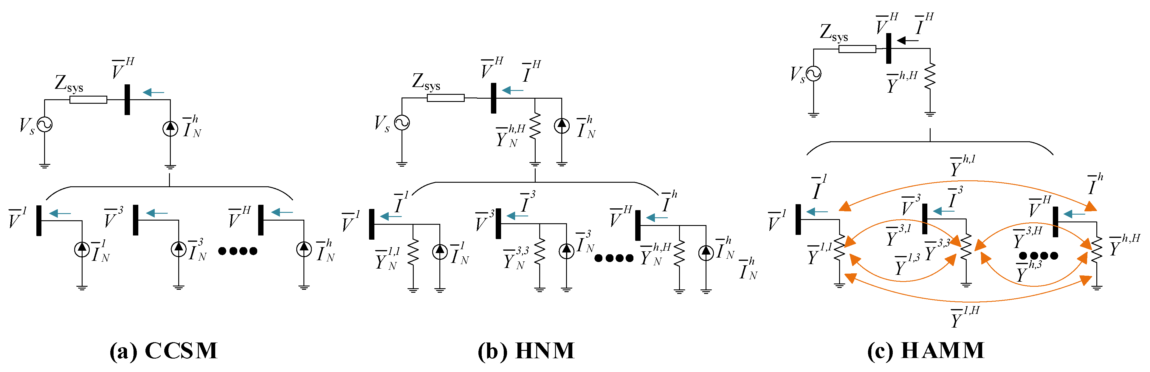
2.1. Conventional HAM Derivation Approach

The mathematical expression of HAMM can be written as (1), representing the correlations between the voltage and current harmonics at the PoC of a PV system with constant operating power.

$$\left[\begin{array}{c}{\overline{I}}_1\\ {\overline{I}}_2\\ {\overline{I}}_3\\ ⋮\\ {\overline{I}}_h\end{array}\right]=\left[\begin{array}{ccccc}{\overline{Y}}_{1,1}& {\overline{Y}}_{1,2}& {\overline{Y}}_{1,3}& \cdots & {\overline{Y}}_{1,H}\\ {\overline{Y}}_{2,1}& {\overline{Y}}_{2,2}& {\overline{Y}}_{2,3}& \cdots & {\overline{Y}}_{2,H}\\ {\overline{Y}}_{3,1}& {\overline{Y}}_{3,2}& {\overline{Y}}_{3,3}& \cdots & {\overline{Y}}_{3,H}\\ ⋮& ⋮& ⋮& \ddots & ⋮\\ {\overline{Y}}_{h,1}& {\overline{Y}}_{h,2}& {\overline{Y}}_{h,3}& \cdots & {\overline{Y}}_{h,H}\end{array}\right]\times \left[\begin{array}{c}{\overline{V}}_1\\ {\overline{V}}_2\\ {\overline{V}}_3\\ ⋮\\ {\overline{V}}_H\end{array}\right]$$

(1)

where ${\overline{I}}_h$ and ${\overline{V}}_H$ are the individual complex current and voltage harmonics at PoC; the HAM element ${\overline{Y}}_{k,j}$ represents the influence of jth voltage harmonic on the kth current harmonic.

Conventionally, the derivation of HAM requires performing the individual voltage harmonic sensitivity tests (or the so-called “fingerprint tests”) on the considered device under a fully controllable voltage source, as in [21,22]. Specifically, the device is first tested under ideally sinusoidal voltage with varying voltage magnitudes. This step is to investigate the impact of the fundamental voltage component on the harmonic current spectrum. Then, individual harmonic is superimposed on the ideal supply voltage with a stepwise adjustment of harmonic voltage magnitudes and phase angles, as illustrated in Figure 5. This step is to investigate the impact of individual voltage harmonic on the harmonic current spectrum. As the output current of the PV system is power-dependent, the PV system has to be kept at a constant operating power to avoid the impact of operating powers on the current harmonic spectrum. Accordingly, a PV panel emulator (in the form of a programmable dc source) has to be applied in order to regulate the operating power of the PV system, while a programmable ac voltage source has to be applied for the harmonic sensitivity tests.

The derivation process of HAM from the harmonic sensitivity tests is given below. It should be noted that (1) can be rewritten as (2), indicating that the hth current harmonic, ${\overline{I}}_h$, is determined by both the fundamental voltage, ${\overline{V}}_1$, and all the voltage harmonics ${\overline{V}}_H$ (H ≠ 1). It is also noticed that ${\overline{Y}}_{h,1}$ can be calculated from ${\overline{I}}_h$ and ${\overline{V}}_1$ when the PV system is tested under ideal supply voltage, as in (3). When the modelled device is tested under any individual supply voltage harmonic, ${\overline{V}}_H$, (2) is simplified into (4), where ${\overline{Y}}_{h,H}$, can be directly calculated from the measurements.

$$\left[\begin{array}{c}{\overline{I}}_1\\ {\overline{I}}_2\\ {\overline{I}}_3\\ ⋮\\ {\overline{I}}_h\end{array}\right]=\left[\begin{array}{c}{\overline{Y}}_{1,1}\\ {\overline{Y}}_{2,1}\\ {\overline{Y}}_{3,1}\\ ⋮\\ {\overline{Y}}_{h,1}\end{array}\right]{\overline{V}}_1+\left[\begin{array}{cccc}{\overline{Y}}_{1,2}& {\overline{Y}}_{1,3}& \cdots & {\overline{Y}}_{1,H}\\ {\overline{Y}}_{2,2}& {\overline{Y}}_{2,3}& \cdots & {\overline{Y}}_{2,H}\\ {\overline{Y}}_{3,2}& {\overline{Y}}_{3,3}& \cdots & {\overline{Y}}_{3,H}\\ ⋮& ⋮& \ddots & ⋮\\ {\overline{Y}}_{h,2}& {\overline{Y}}_{h,3}& \cdots & {\overline{Y}}_{h,H}\end{array}\right]\times \left[\begin{array}{c}{\overline{V}}_2\\ {\overline{V}}_3\\ {\overline{V}}_4\\ ⋮\\ {\overline{V}}_H\end{array}\right]$$

(2)

$${\overline{Y}}_{h,1}={\overline{I}}_h/{\overline{V}}_1$$

(3)

$${\overline{Y}}_{h,H}=({\overline{I}}_h-{\overline{Y}}_{h,1}{\overline{V}}_1)/{\overline{V}}_H$$

(4)

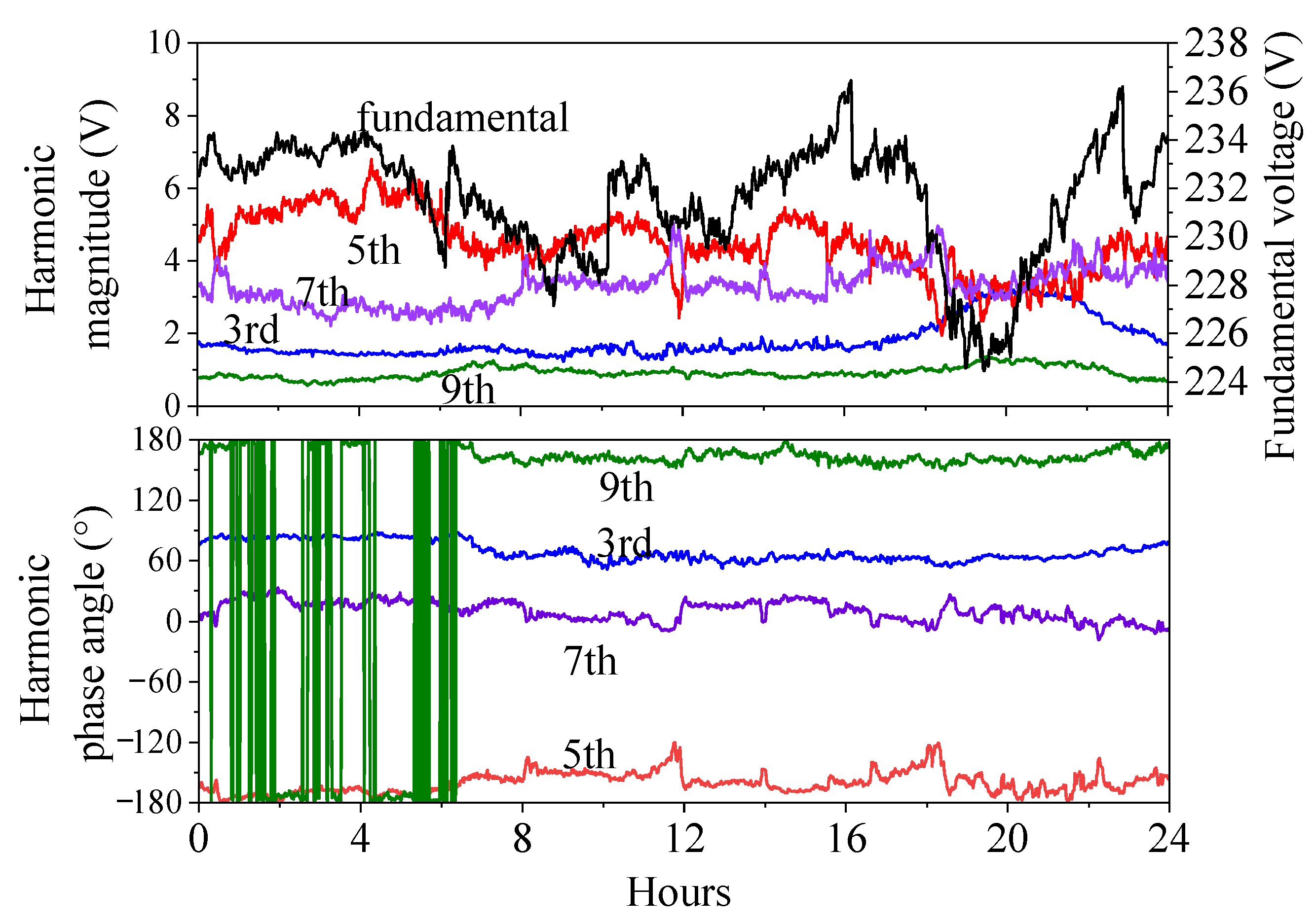
2.2. Harmonic Generation and Grid Interaction Mechanism of Rooftop PV Systems

Before applying HAMM to the PV systems, the harmonic generation and grid interaction mechanisms have to be investigated. Figure 6 is the generalized circuit topology of a single-phase rooftop PV system, which consists of a PV panel, a dc-link capacitor, C_dc, a full-bridge inverter and LC filter for harmonic suppressing [23]. According to the KCL principle, the grid-side current, i_g, can be expressed as (5). As the LC filter capacitor, C_f, has a relatively small value, (5) can be simplified as (6). By applying a Fourier transform to (6), the grid-side current, i_g, can be divided into a fundamental current, $i_g^1$, and the harmonic currents, ${\displaystyle \sum i_g^h}$, as in (7). It is noticed that the harmonic current, $i_g^h$, is mainly determined by the inverter output voltage harmonic, $v_{inv}^h$ and the grid supply voltage harmonic, $v_g^h$, which is uncontrollable. To further investigate the features of $v_{inv}^h$, the inverter output voltage, v_inv, can be expressed as the dc-link voltage, v_dc, multiplied by the PWM pulse signal, d, as in (8). It should be noted that the harmonic contents of the PWM pulse signal, d^h, is determined by the PWM strategy being applied. It can be concluded from (8) that $v_{inv}^h$ is determined by the dc-link voltage variation, ${\tilde{v}}_{dc}$, and the PWM pulse signal harmonics, d^h.

To establish the connection between the dc-link voltage, v_dc, and the grid-side current, i_g the power output of the PV panels, p_inv, and the power injected into the power grid, p_g, can be expressed as (9) and (10), respectively (here, a unit power factor is assumed). As the power losses for the power conversion stage are relatively small as opposed to the total power generated, it is assumed that p_inv equals p_g, (also $V_g^1{I}_g^1\approx v_{dc}{i}_{pv}$); therefore, (11) can be derived. It is noticed from (11) that ${\tilde{v}}_{dc}$ brings in even harmonic content twice the frequency of the grid, 2w₀. It is also noticed that ${\tilde{v}}_{dc}$ (and hence $v_{inv}^h$ in (8)) is power-dependent. In addition, $\left|{\tilde{v}}_{dc}\right|$ will be reduced with the decreasing operating power of PV systems. Accordingly, ${\tilde{v}}_{dc}$ is characterized by the odd harmonics with the angular frequency equaling (2k + 1)w₀ (k is a positive integer number), and the odd harmonics will also be observed from v_inv, as in (8). Therefore, the harmonic generation and grid interaction mechanism of PV systems can be summarized as follows: (1) the PV systems mainly generate odd harmonics; (2) the harmonic emission level of PV systems is mainly determined by the PWM strategy being applied, the background supply voltage distortions and the system operating power.

$$i_g={\displaystyle \int \frac{v_{inv}-v_g}{L_f}}dt-C_f{\dot{v}}_g$$

(5)

$$i_g={\displaystyle \int \frac{v_{inv}-v_g}{L_f}}dt$$

(6)

$$i_g=i_g^1+{\displaystyle \sum _{h=2}^N{i}_g^h}=\frac{1}{L_f}{\displaystyle \int (v_{inv}^1-v_g^1)}dt+\frac{1}{L_f}{\displaystyle \int ({\displaystyle \sum _{h=2}^N{v}_{inv}^h}-{\displaystyle \sum _{h=2}^N{v}_g^h})}dt$$

(7)

$$v_{inv}=v_{inv}^1+{\displaystyle \sum _{h=2}^N{v}_{inv}^h}=d{v}_{dc}=d^1{V}_{dc}+(d^1{\tilde{v}}_{dc}+V_{dc}{\displaystyle \sum _{h=2}^N{d}^h}+{\tilde{v}}_{dc}{\displaystyle \sum _{h=2}^N{d}^h})$$

(8)

$$p_g=v_g^1{i}_g^1=V_g^1{I}_g^1[1+\cos (2w_{0}t)]$$

(9)

$$p_{dc}=v_{dc}{i}_{pv}-v_{dc}{C}_{dc}\frac{d{v}_{dc}}{dt}=v_{dc}{i}_{pv}-v_{dc}{C}_{dc}\frac{d{\tilde{v}}_{dc}}{dt}$$

(10)

$${\tilde{v}}_{dc}=-{\displaystyle \int [\frac{V_g^1{I}_g^1}{C_{dc}{V}_{dc}}}{v}_{dc}{i}_{pv}\cos (2w_{0}t)]dt$$

(11)

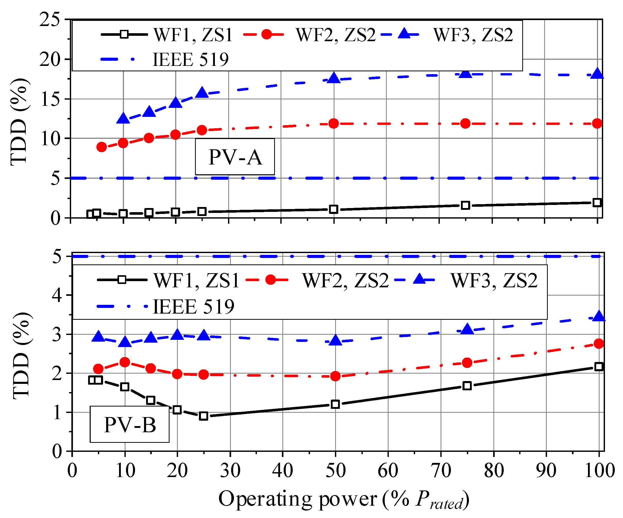
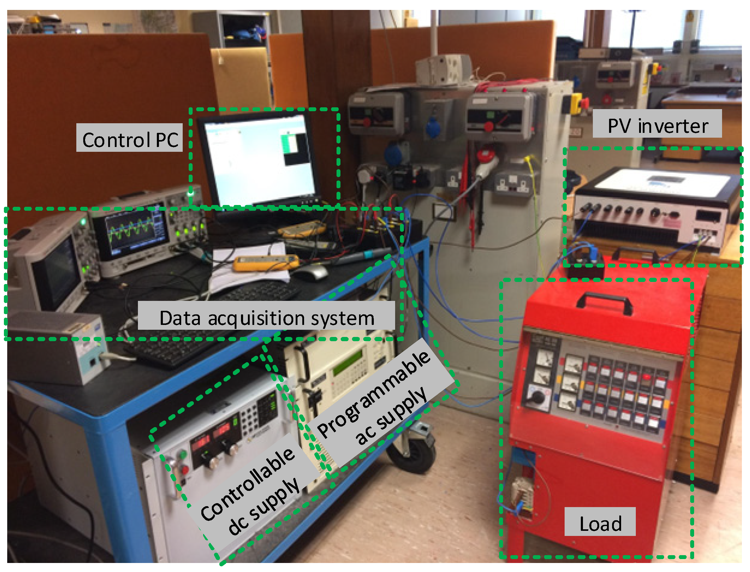
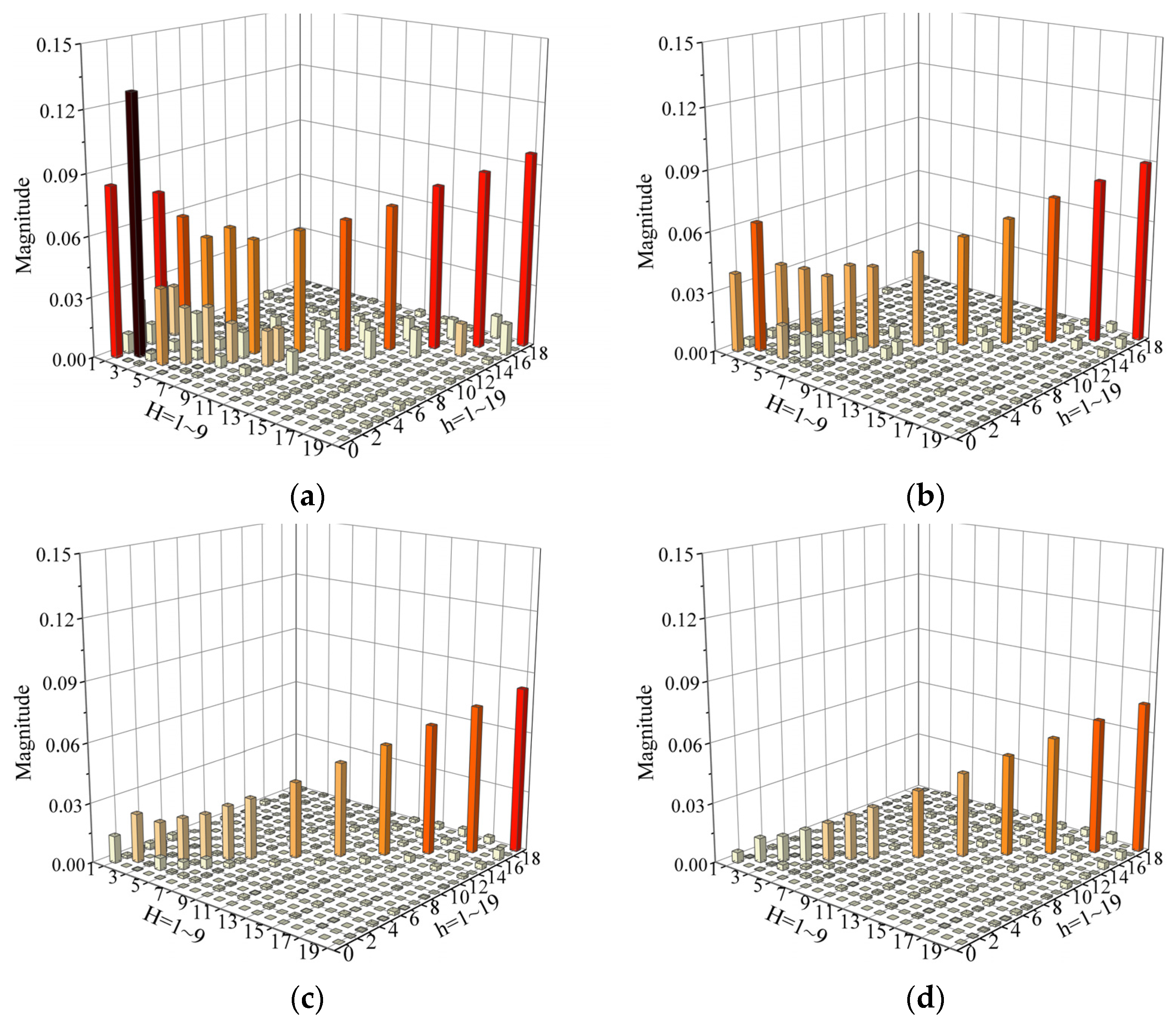
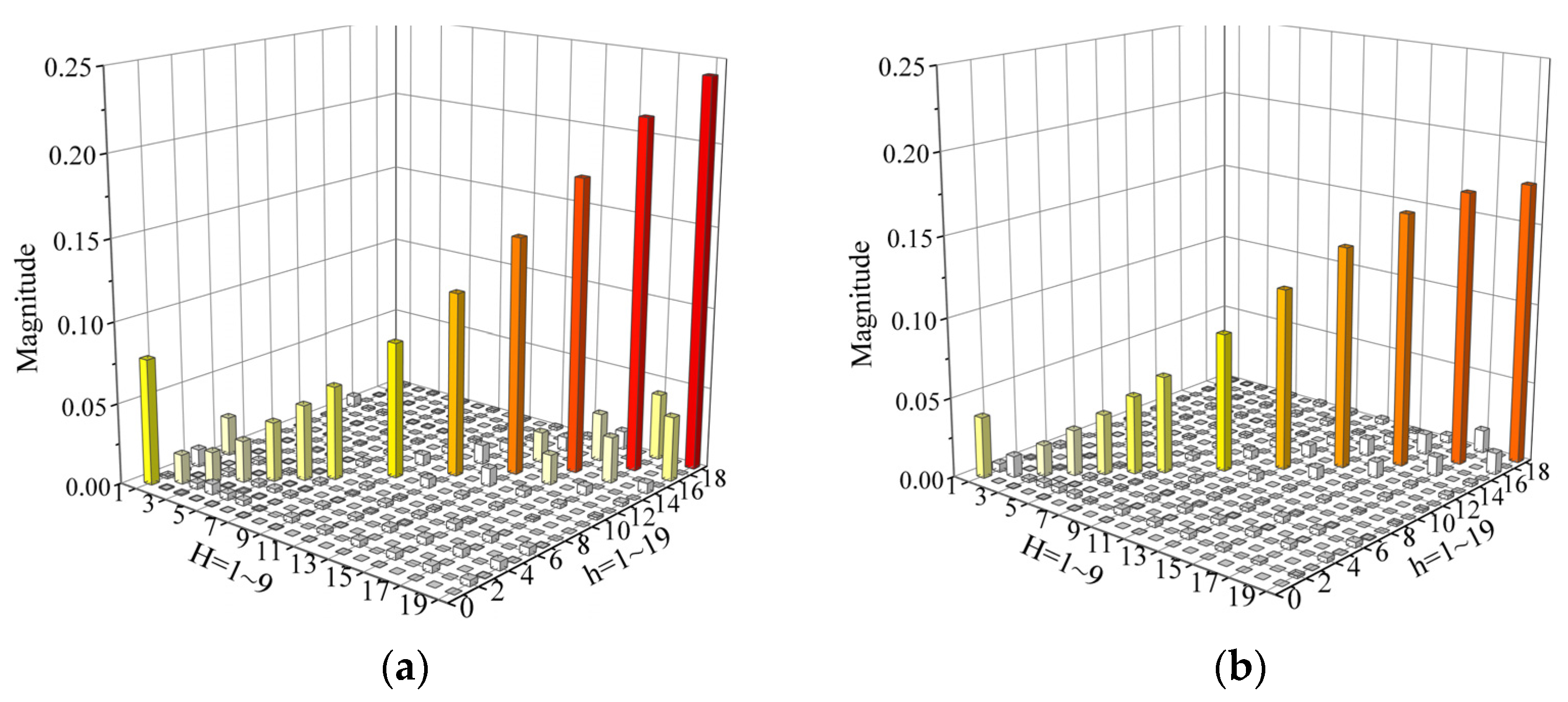
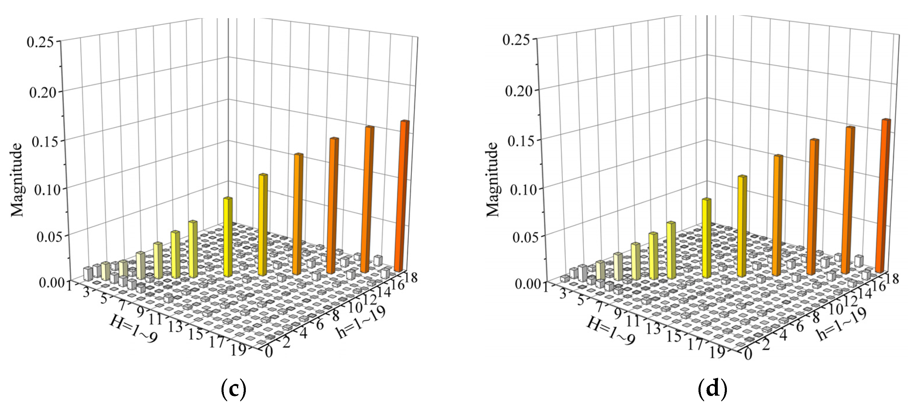
2.3. The Power Dependency Evalution of HAM by Laboratory Tests

The analytical analysis performed in Section 2.2 indicates that there exist inherent correlations between harmonic distortion characteristics (and hence HAM) at different powers. To further investigate the power dependency of HAM for PV systems, a testbed is set up as in Figure 7, consisting of a fully programmable ac supply (capable of generating defined supply voltage harmonics), a controllable dc supply (capable of providing defined constant power to the PV inverter), single-phase residential PV systems, data acquisition system and a control PC. With the aid of the testbed, the harmonic sensitivity tests are performed on two single-phase PV systems with their basic information tabulated in

Table 1. Basic information of the two single-phase PV systems.

Inverter	PV-A	PV-B
Technology	Transformerless	With low-frequency transformer
Rated power (kVA)	4.6	4.6
Phase connection	Single-phase	Single-phase
Rated/reference current (A)	20	20

. Specifically, the individual harmonic tests are performed for PV-A and PV-B operating at 100% P_rated down to 10% P_rated (with a step of 10% P_rated). For each test, only one individual voltage harmonic is superimposed on the fundamental sinusoidal supply voltage, with a combination of different harmonic magnitudes and phase angles. The considered individual voltage harmonics include even harmonics from 2 to 6, and odd harmonics from 3 to 19. Their harmonic magnitudes vary from a tenth of the individual harmonic limits (denoted as V_h,limit) given in [8] to 1.2 × V_h,limit (for 0.8 × V_h,limit PVI-C) with a step of V_h,limit/10, while the harmonic phases increase from 0° to 360° with a step of 30°. During the individual harmonic tests, the rms value of the resultant supply voltage waveform is maintained at 1 pu (i.e., 230 V). All the test points are programmed as testing sequences in MATLAB, while the communication between the testbed and control PC is achieved by using SCPI commands via RS232 and GPIB remote interface.

By applying the conventional HAM derivation approach in Section 2.1 to the measurements obtained from the harmonic sensitivity tests, the HAMs for the tested PV systems operating at different powers can be derived, with their magnitudes displayed in Figure 8 and Figure 9. It is noticed that the dominant elements of the HAM matrix are those on the diagonal, implying the current harmonics of PVIs are mainly determined by the voltage harmonics at the same order. This is attributed to the waveform shaping capability of PWM strategies applied to PV inverters, meaning that PV systems are characterized by low nonlinearity.

Moreover, the distribution patterns of HAMs exhibit strong similarity at different powers, which is also proved by the analytical analysis in Section 2.2. Here, the Pearson correlation coefficient, ρ, is used to quantify the correlation of HAMs at different powers, as illustrated in Figure 10. It turns out that a strong linear correlation (ρ > 0.98) exists between HAMs at adjacent powers, implying the feasibility of HAM interconversion. Additionally, the linear correlation of HAMs at different powers deteriorates with the increasing power difference. The above power-dependency features of PVs’ HAMs are the basis for proposing the practical HAM derivation approach in the next section.

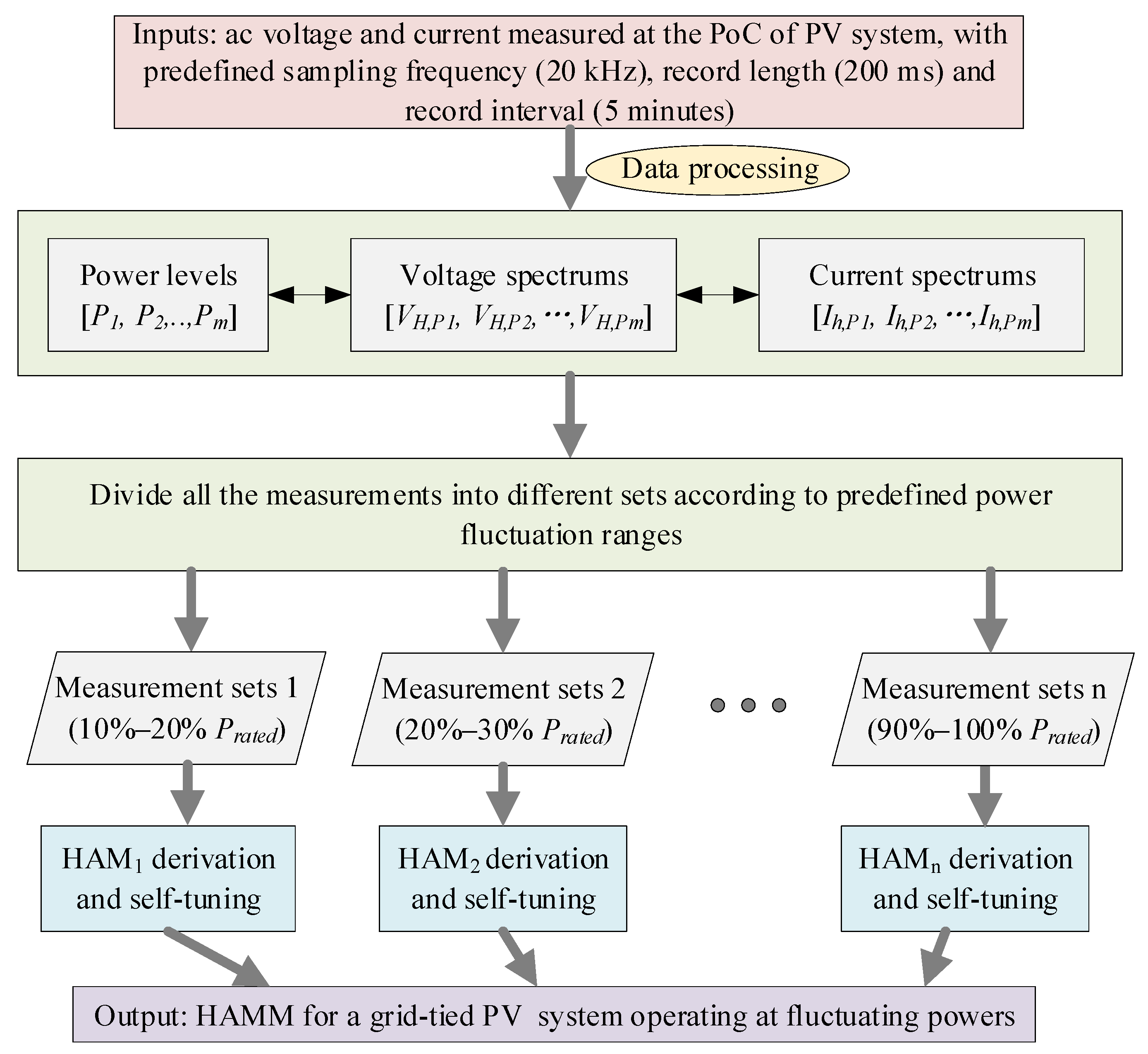
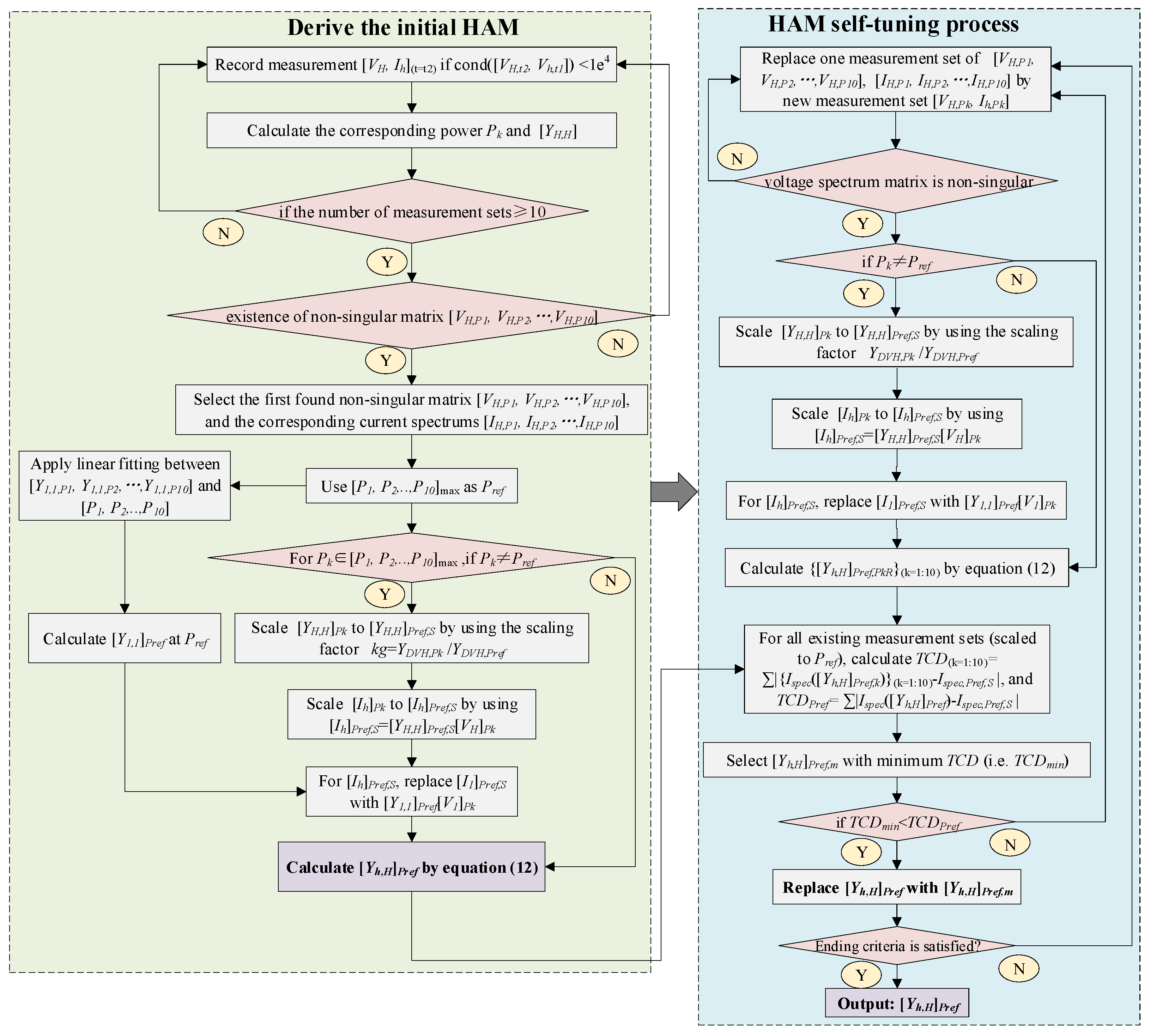
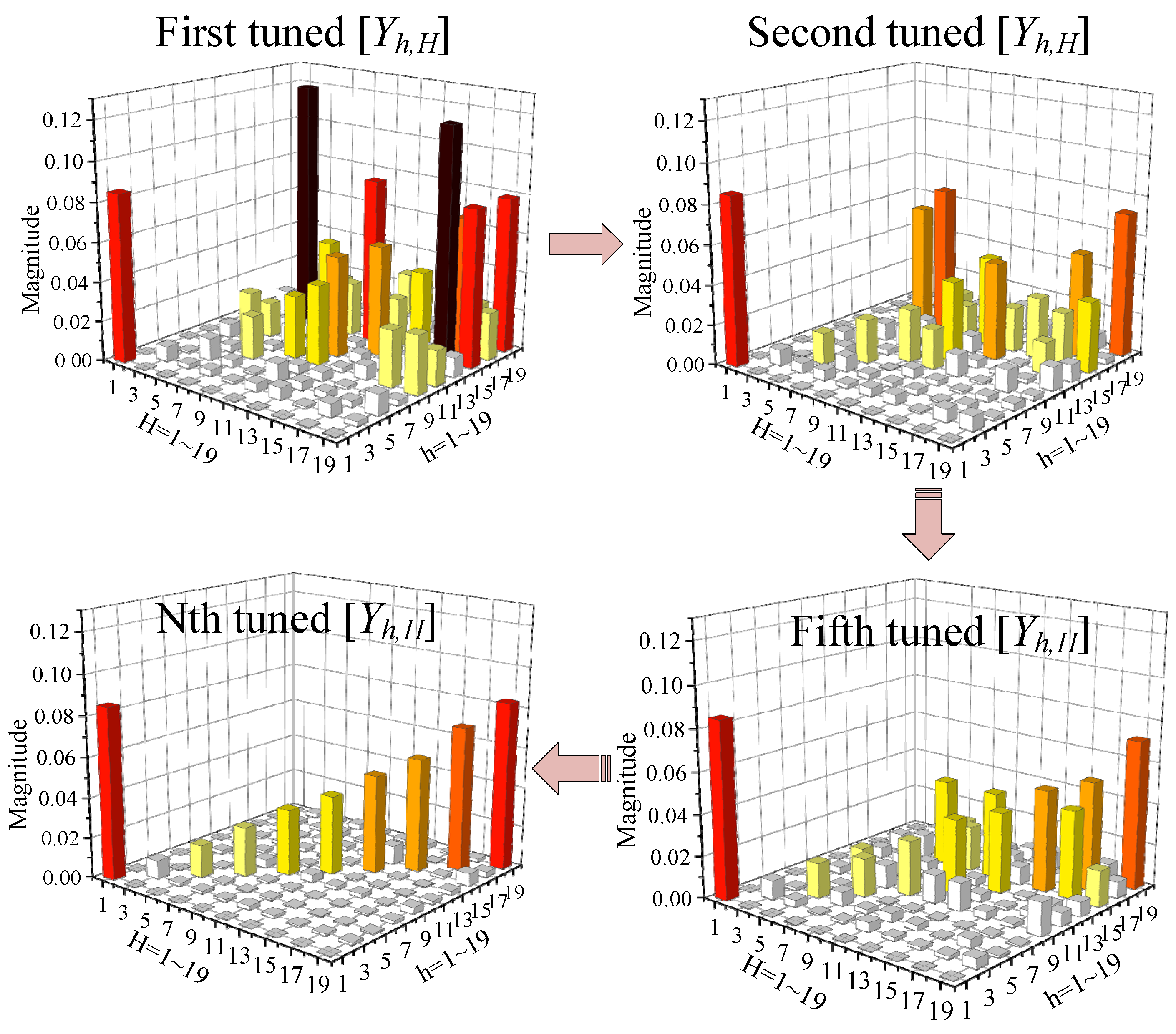
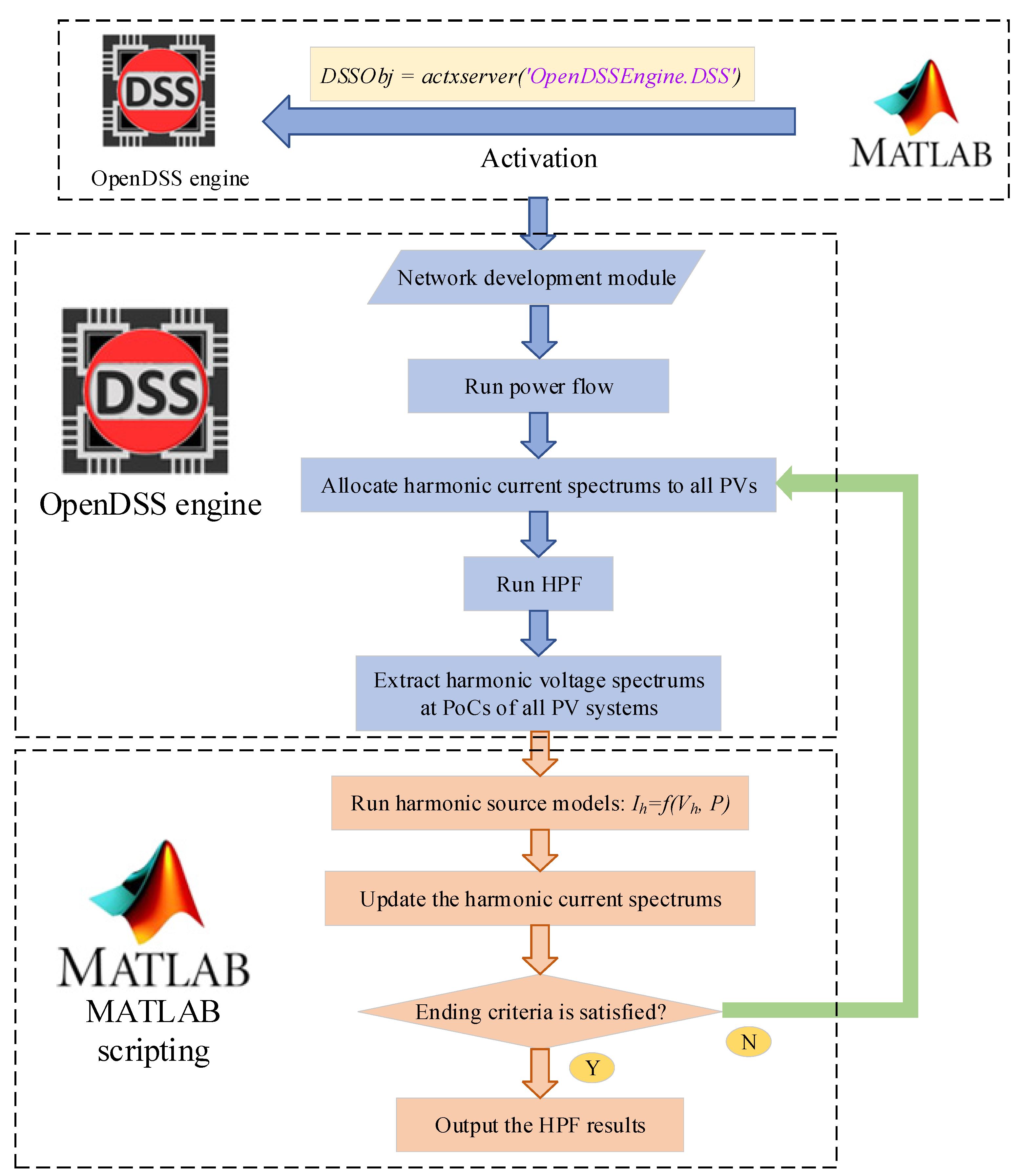
2.4. The Practical HAM Derivation Approach for Fluctuating Power PV Systems

As in Section 2.3, the conventional HAM derivation approach is based on the harmonic sensitivity tests performed on a PE device with constant operating power, which is infeasible to be applied to a PV system that operates under real-grid conditions. As it is affected by the solar irradiation and weather conditions, the daily operating power of a practical grid-tied PV system normally varies from 10% P_rated to 100% P_rated [11]. As the HAMs exhibit strong linear correlations at adjacent powers, the voltage and current waveforms captured at the PoC of a grid-tied PV system operating during a typical day can be applied for the HAM derivation. Specifically, as in Figure 11, the voltage and current waveforms of a grid-tied PV system are recorded with predefined sampling frequency, length and interval. After the one-day measurements are captured, they are firstly sorted from highest power to lowest power, and then divided into different sets according to the equally distributed power ranges. For the measurement sets within each power range, they are applied for the HAM derivation and self-tuning. The final outputs are the HAMs at different powers. The practical HAM derivation process based on the infield measurements within each power range is further explained in the following section.

As explained in Section 2.2, PV systems mainly generate odd harmonics; hence, only odd harmonics will be considered for the HAM derivation. Additionally, only harmonic orders upper to 19th are considered, as any higher harmonic order has negligible magnitude. According to (1), the calculation of ${\overline{Y}}_{h,H}$ (h, H = 1, 3, 5,…, 19) requires at least 10 measurement sets captured at the same power and the formed voltage matrix has to be non-singular, as in (12).

$$\left[\begin{array}{cccc}{\overline{Y}}_{1,1}& {\overline{Y}}_{1,3}& \cdots & {\overline{Y}}_{1,19}\\ {\overline{Y}}_{3,1}& {\overline{Y}}_{3,3}& \cdots & {\overline{Y}}_{3,19}\\ ⋮& ⋮& \ddots & ⋮\\ {\overline{Y}}_{19,1}& {\overline{Y}}_{19,3}& \cdots & {\overline{Y}}_{19,19}\end{array}\right]=\left[\begin{array}{cccc}{\overline{I}}_1^1& {\overline{I}}_1^2& \cdots & {\overline{I}}_1^{10}\\ {\overline{I}}_3^1& {\overline{I}}_3^2& \cdots & {\overline{I}}_3^{10}\\ ⋮& ⋮& \ddots & ⋮\\ {\overline{I}}_{19}^1& {\overline{I}}_{19}^2& \cdots & {\overline{I}}_{19}^{10}\end{array}\right]/\left[\begin{array}{cccc}{\overline{V}}_1^1& {\overline{V}}_1^2& \cdots & {\overline{V}}_1^{10}\\ {\overline{V}}_3^1& {\overline{V}}_3^2& \cdots & {\overline{V}}_3^{10}\\ ⋮& ⋮& \ddots & ⋮\\ {\overline{V}}_{19}^1& {\overline{V}}_{19}^2& \cdots & {\overline{V}}_{19}^{10}\end{array}\right]$$

(12)

According to the findings in Section 2.3, HAMs at adjacent powers exhibit strong linear correlations with a Pearson correlation coefficient close to one; it is assumed that within each power range, HAM at power P_k can be represented as HAM at P_ref multiplied by a scaling factor k_g, i.e., HAM_Pk = k_g × HAM_Pref. In this way, the measured current spectrums with powers different to P_ref can all be scaled to their corresponding values at P_ref, which will then be applied to (12) for calculating the initial HAM_Pref. Afterwards, the parameter values of HAM_Pref will be self-tuned until the lowest THD errors are achieved for all the measurements within the specified power range.

The detailed HAM derivation and self-tuning process are made up of the following steps, with the flowchart given in Figure 12:

For Step (1) for any captured voltage and current waveforms within the selected power fluctuation range, record the corresponding spectrums [V_H,I_h]_(t=t2) to the database if the condition number is between [V_H]_(t=t2) and the former saved voltage spectrum [V_H]_(t=t1) is below the predefined threshold value (e.g., 1 × 10⁴); calculate the operating power P_k and the estimated [Y_H,H]_Pk from the saved spectrums by using [Y_H,H]_Pk = [I_H]_Pk/[V_H]_Pk;

For Step (2), find the first non-singular voltage spectrum matrix [V_H,P1, V_H,P2, …, V_H,P10] and the corresponding current spectrum matrix [I_H,P1, I_H,P2, …, I_H,P10] after the number of captured measurement sets is above 10, and take the maximum operating power as the refence power level, P_ref; mark the data sets as [VI]_{spec_ns};

For Step (3) for any selected measurement set, [V_H, I_h]_Pk, within the 10 measurement sets of the [VI]_{spec_ns} scale, its estimated [Y_H,H]_Pk from P_k to P_ref if P_k is not equal to P_ref (i.e., [Y_H,H]_Pref,S = [Y_H,H]_Pk/k_g); the scaling factor k_g is applied by assuming that the power dependencies of [Y_H,H] have the same trend for all considered odd harmonics; k_g is calculated from the Y_DVH,Pk divided by Y_DVH,Pref, where the subscript DVH refers to the common dominant voltage harmonic order between [V_H]_Pk and [V_H]_Pref;

For Step (4), scale the current spectrum [I_h]_Pk from P_k to P_ref by using equation [I_h]_Pref,S = [Y_H,H]_Pref,S × [V_H]_Pk; calculate Y_1,1,Pref at P_ref by applying the linear interpolation between [Y_1,1,P1, Y_1,1,P2, …, Y_1,1,P10] and [P₁, P₂, …, P₁₀]; replace [I₁]_Pref,S by [Y_1,1]_Pref × [V₁]_Pk;

For Step (5), repeat steps 3–4 until all the 10 current spectrums of [VI]_{spec_ns} are scaled to their counterparts at P_ref and calculate the [Y_h,H]_Pref (i.e., HAM at P_ref) from (12); the initially obtained [Y_h,H]_Pref will be applied for further parameter self-tuning process;

For Step (6) for any new measurement set [V_H,I_h]_Pk, use it to replace any measurement set within [VI]_{spec_ns} and check if the updated voltage spectrum matrix is ill-conditioned; for any non-singular voltage spectrum matrix, scale [I_h] from P_k to its counterpart at P_ref if P_k does not equal P_ref and calculate the new HAM, [Y_h,H]_Pref,k by (12) (with same calculation procedures specified in steps 4–5);

For Step (7), calculate the total current difference TCD_(k=1:10) by using equation TCD_(k=1:10) = ∑∑|I_spec([Y_h,H]_Pref,k) − I_spec,Pref,S|, where I_spec([Y_h,H]_Pref,k) refers to the current spectrum calculated by using [Y_h,H]_Pref,k and I_spec,Pref,S represents the current spectrum scaled to Pref; calculate the TCD at P_ref, TCD_Pref by using TCD_Pref = ∑∑|I_spec([Y_h,H]_Pref) − I_spec,Pref,S)|; within all the available [Y_h,H]_{Pref,k(k=1:10)}, select [Y_h,H]_Pref,m with minimum TCD (i.e., TCD_min); replace [Y_h,H]_Pref with [Y_h,H]_Pref,m if TCD_min is smaller than TCD_Pref;

For Step (8), repeat steps 6–7 until the ending criteria is met (e.g., the variation in HAM’s norm is below the threshold value); output the fine-tuned [Y_h,H]_Pref representing the estimated HAM at P_ref.

The HAM self-tuning process is illustrated in Figure 13. It is observed that the finely-tuned HAM exhibits a distribution pattern similar to the one derived from the harmonic sensitivity tests, which further demonstrates the feasibility of the proposed approach. By applying the above HAM derivation and self-tuning approach to the measurements of each partitioned power range (as indicated in Figure 11), HAMs at different reference powers are obtained from the infield measurements of a grid-tied PV system and form the HAMM. Finally, a linear interpolation approach is applied to estimate the HAM at a power that is different to the selected reference powers.

3. Results and Discussions

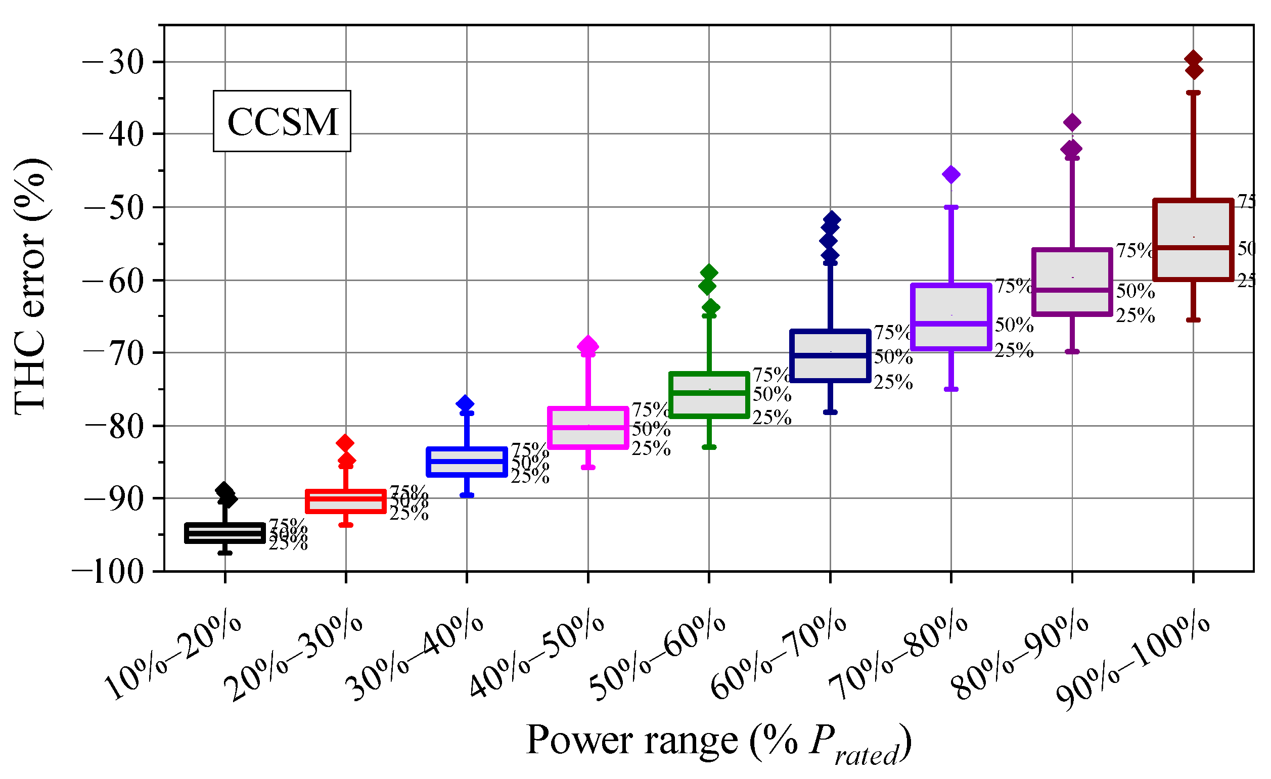
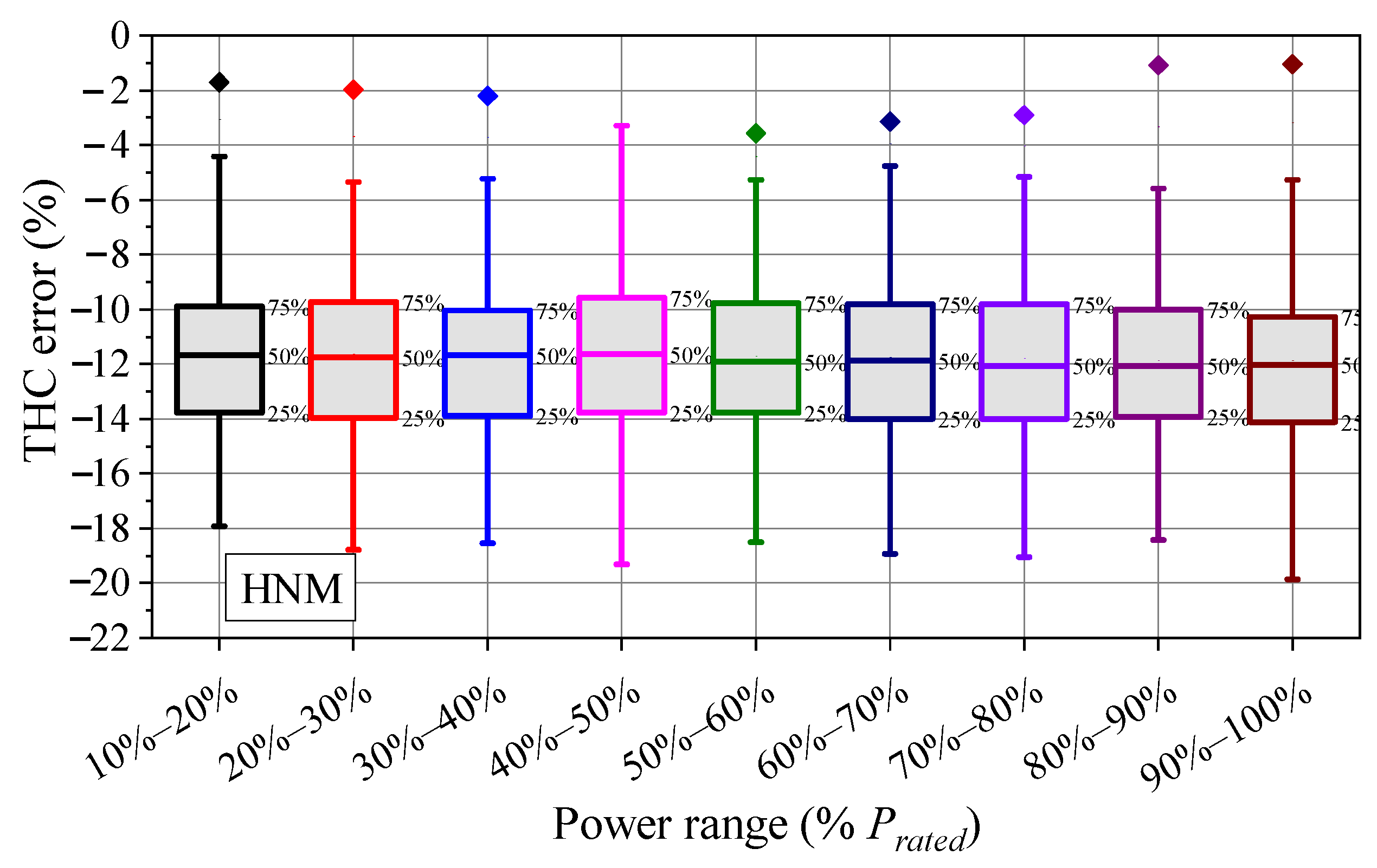
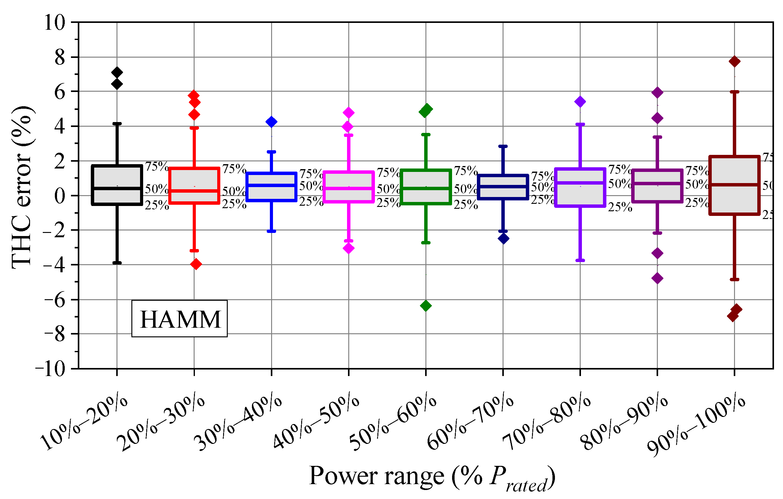
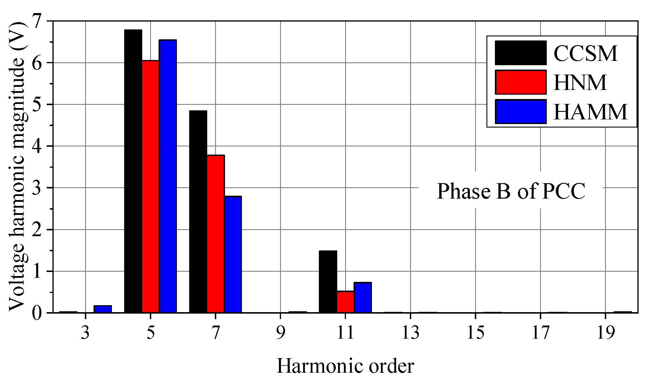
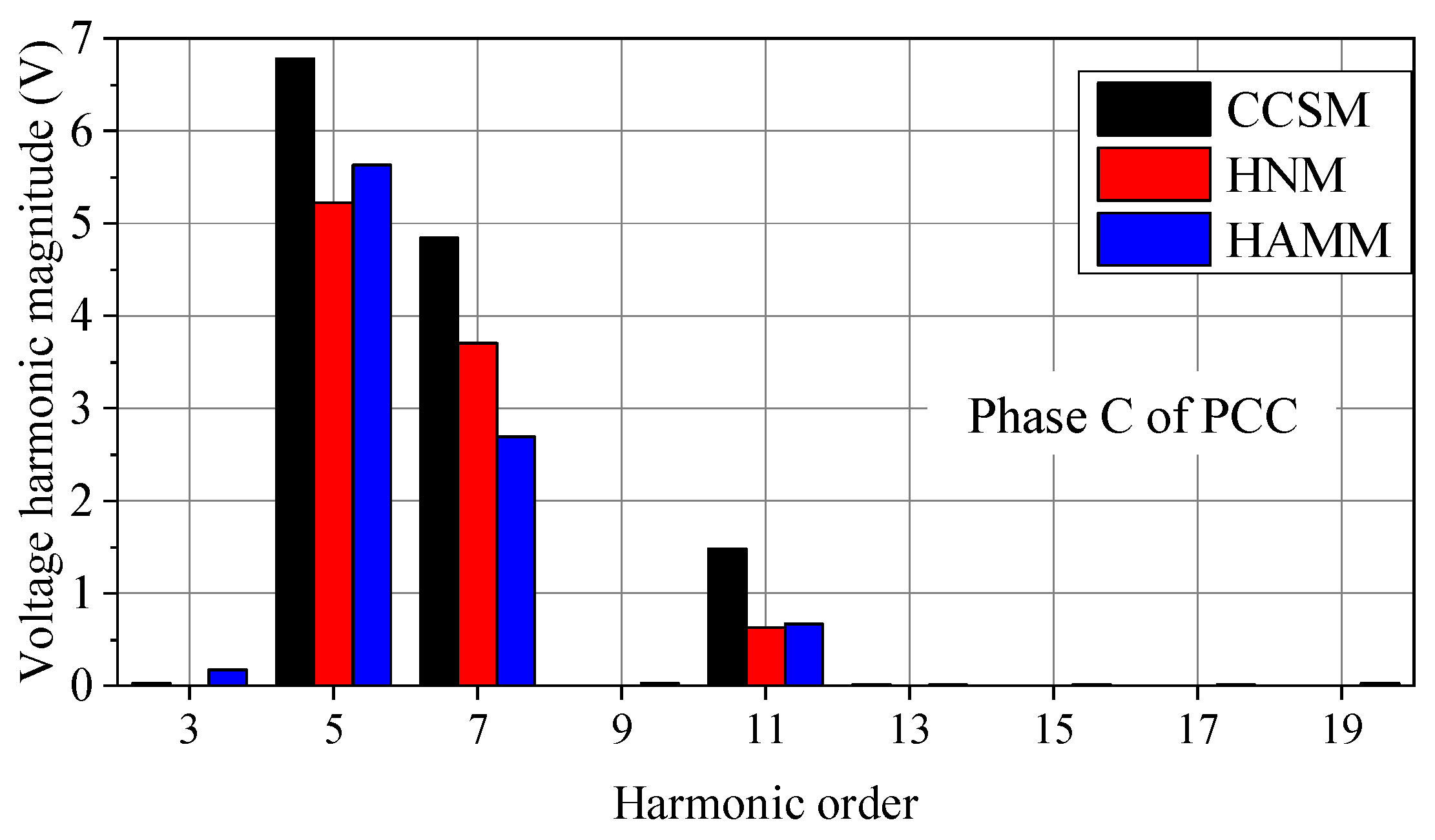
3.1. Accuracy Comparison among CCSM, HNM and HAMM

To evaluate the accuracy of the proposed HAM derivation approach, additional laboratory tests are performed on PV-A based on the testbed introduced in Section 2.3, and then CCSM, HNM and HAMM are developed for PV-A operating under a combination of different powers and different supply voltage distortions. Specifically, the typical operating power range of a grid-tied PV system, 10%~100% P_rated, is partitioned into 9 power ranges with a fixed power band equaling 10% P_rated. Within each power range, 100 tests made up of randomly selected operating powers and supply voltage distortions are applied to PV-A via the testbed, and the recorded voltage and current waveforms are applied for developing HAMM for PV-A. The current spectrum of PV-A operating at P_rated with sinusoidal supply voltage is used as the CCSM for PV-A. To develop HNM for PV-A, the current spectrum for CCSM is used as the harmonic current source of HNM, while the parallel-connected Norton impedance of HNM is determined from the harmonic sensitivity tests in Section 2.3. Unlike HNM and HAMM, CCSM does not consider the power dependency of PV-A’s harmonic emission characteristics. The total harmonic current (THC) errors between all the measurements and simulation results are computed using (13) and (14), with the results represented as box plots in Figure 14, Figure 15 and Figure 16.

$$THC=\sqrt{{\displaystyle \sum _{h=3}^{19}{I}_h^2}} (h=3, 5, \dots ,19)$$

(13)

$$TH{C}_{err}=\frac{TH{C}_{sim}-TH{C}_{mea}}{TH{C}_{mea}}\times 100\%$$

(14)

It turns out that for CCSM, its THC error gradually increases with the decreasing operating powers of PV-A. As CCSM fully ignores the voltage dependency and power dependency of the harmonic emission characteristics, the application of CCSM can result in unrealistic simulation results. Compared with CCSM, HNM has improved accuracy, as its THC errors generally kept within −10% and −14% for the whole power range. HAMM achieves the best accuracy among the three harmonic modelling approaches, with the THC errors mainly fluctuating between −2% and 2% for the whole power range.

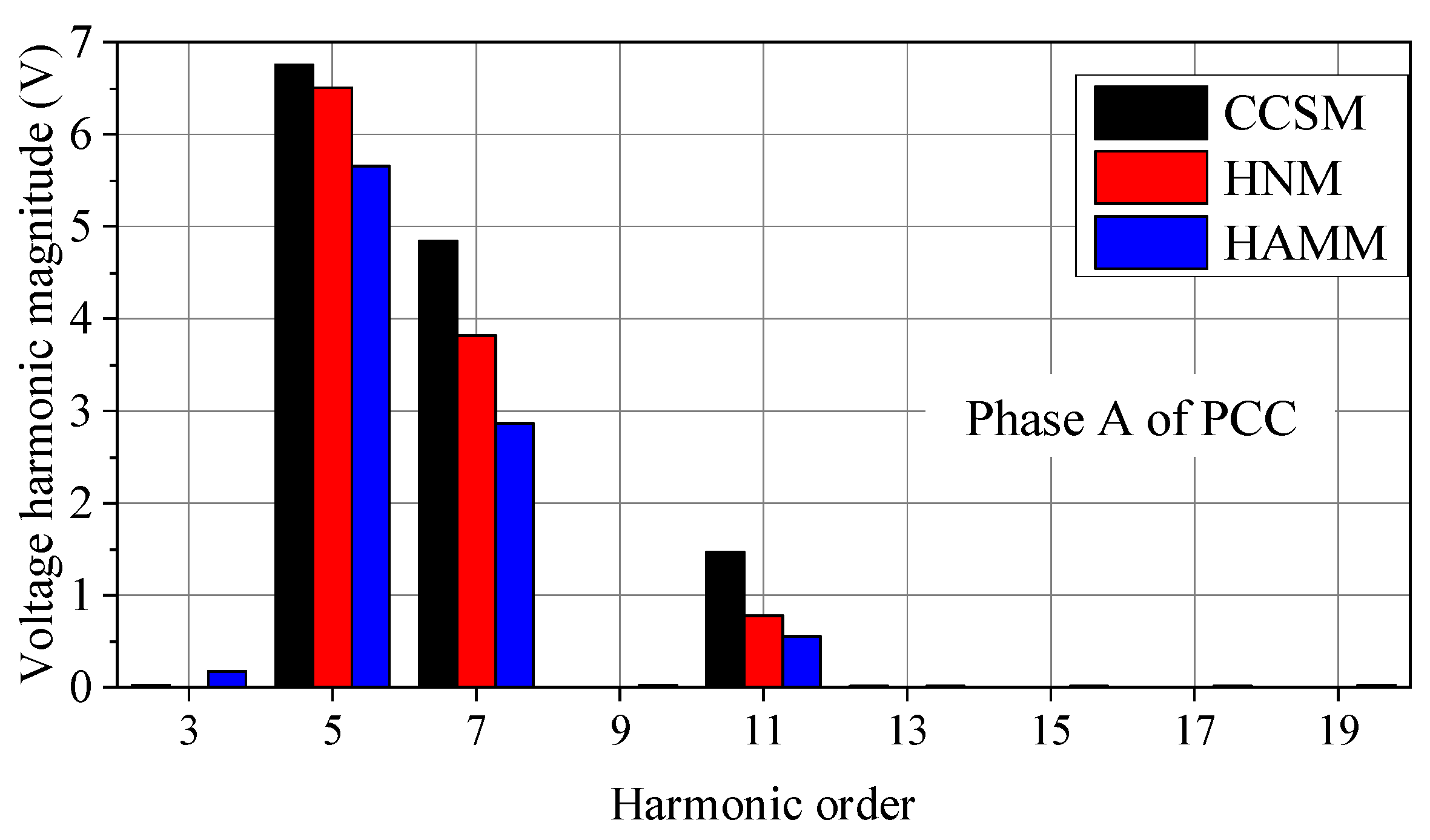
3.2. Comparison of Harmonic Power Flow Results among CCSM, HNM and HAMM

Based on the accuracy assessment of HAMM in Section 3.1, it can be concluded that HAMM has better performance in harmonic source representation of fluctuating-power PV systems as opposed to CCSM and HNM, due to its capability of properly considering the voltage and power dependencies of harmonic currents. In this section, the impact of harmonic source model selection on the harmonic power flow (HPF) analysis is investigated, since HPF is an important tool for assessing the power quality impact of large-scale PV integration [2]. Here, a European low voltage test feeder is simulated in OpenDSS, with the network topology illustrated in Figure 17. The basic information of the test feeder can be found in [24]; hence, it is not repeated here.

To evaluate the harmonic impact of PV systems on the supply voltage distortion at the point of common coupling (PCC), five groups of single-phase PV systems are connected to the test feeder, with their grid integration points illustrated in Figure 17. Each group of PV systems are made up of five PV-As, with their aggregated power equaling 23 kW. As the harmonic sources in OpenDSS are modelled as harmonic currents, a co-simulation approach between MATLAB and OpenDSS is utilized in order to integrate CCSM, HNM and HAMM into the OpenDSS HPF solver, as in Figure 18. Specifically, it starts with the network model development in the OpenDSS engine, followed by activating its COM interface in MATLAB. Afterwards, a snapshot power flow is executed to initiate the grid state variables (i.e., voltage magnitudes and phase angles at all nodes), and all the harmonic current sources are initiated with their corresponding harmonic current spectrums measured under the ideal supply condition. After executing HPF, the harmonic voltage spectrums at PoCs of all the PV systems can be extracted and fed to CCSM, HNM and HAMM as their input data. By running the harmonic source models in MATLAB, their output harmonic current spectrums will be used to update the original ones allocated to all PV systems in OpenDSS. By executing the OpenDSS HPF solver, the supply voltage harmonics at all nodes are updated. The above iterative process is repeated until the ending criteria are met (e.g., the maximum number of iterations is met or the variation in voltage THD at PCC is below 1%). With the aid of the proposed co-simulation approach, the harmonic penetration analysis of PV systems with CCSM, HNM and HAMM is performed, with the simulated voltage harmonics at PCC provided in Figure 19, Figure 20 and Figure 21. It turns out that the utilization of HAMM for PV systems generally results in lower voltage harmonics at PCC than in the cases of using CCSM and HNM, indicating that the application of CCSM for the harmonic integration analysis of PV systems can result in overestimated results.

4. Conclusions

PV systems are integrated into the distribution networks through power inverters, which are nonlinear power electronic devices that inherently inject harmonics into the grid. Their current harmonic emission characteristics are not only determined by their general circuit topologies and control strategies, but are also affected by the background supply voltage distortions and the device operating powers. To investigate the harmonic integration impact of PV systems, a suitable harmonic source model capable of accurately representing the harmonic emission characteristics of PV systems operating under real grid conditions is required. Accordingly, this paper firstly reviews the conventional harmonic source modelling techniques and their applicability for grid-tied PV systems, with a special focus on the three most widely used frequency-domain modelling approaches, including CCSM, HNM and HAMM. Although HAMM has the best accuracy among all the three methods, its conventional derivation approach relies on the harmonic sensitivity tests with the PV system operating at constant power, and this can only be performed under laboratory conditions. To improve the applicability of HAMM for grid-tied PV systems operating under varying grid conditions and powers, this paper further analytically investigates the harmonic generation and grid interaction mechanisms of rooftop PV systems and obtains the following conclusions: (1) PV systems mainly generate odd harmonics; (2) the generated harmonic current spectrums of PV systems are mainly determined by the PWM strategy being applied, the supply voltage distortions and the device operating power. To further investigate the power dependency of harmonics emitted from PV systems, a fully controllable testbed is set up and based on this, the harmonic sensitivity tests are applied to two different single-phase PV systems operating at selected power levels, with the corresponding derived HAMs. It is noticed that a strong linear correlation exists between HAMs at adjacent powers. Based on this, a HAM derivation and self-tuning approach is proposed to derive the HAMs at different powers from the infield measurements of a grid-tied PV system. According to the accuracy comparison among CCSM, HNM and HAMM, it turns out that HAMM achieves the highest accuracy in the application of harmonic source modelling of PV systems. Finally, this paper proposes a co-simulation approach to compare the HPF results implemented with CCSM, HNM and HAMM, and it is found that using CCSM for the harmonic emission representation of PV systems may overestimate the supply voltage distortion level at PCC. The proposed HAM derivation approach greatly improves the infield implementation capability of HAMM, and has good compatibility with commercial HPF solvers.

References

1. Forson, P.; Samuel, G.; Mark, A.B.; Eric, E.D. Impact assessment of grid tied rooftop PV systems on LV distribution network. Sci. Afr. 2022, 16, e01172. [Google Scholar]
2. Oktoviano, G.; Dhivya, S.K.; Carlos, D.R.; Dipti, S. Review of power system impacts at high PV penetration Part I: Factors limiting PV penetration. Sol. Energy 2020, 210, 181–201. [Google Scholar]
3. Erik, D.J.; Peter, V. The Impact of Large-Scale PV on Distribution Grid Operation and Protection; and Appropriate Testing. In Proceedings of the CIRED 2012 Workshop: Integration of Renewables into the Distribution Grid, Lisbon, Portugal, 29–30 May 2012; pp. 1–4. [Google Scholar]
4. Li, W.; Yang, G.; Zhou, Z.; Lu, Q.; Du, D.; Liu, Y. Impact of the distributed photovoltaic on the current protection of 10kV distribution network. In Proceedings of the 2013 IEEE PES Asia-Pacific Power and Energy Engineering Conference (APPEEC), Hong Kong, China, 8–11 December 2013; pp. 1–4. [Google Scholar]
5. IEEE Standard 1547-2003; IEEE Standard for Interconnecting Distributed Resources with Electric Power Systems. IEEE Standard: New York, NY, USA, 2003.
6. IEC 61727-2004; Photovoltaic (PV) Systems—Characteristics of the Utility Interface. IEC Standard: Geneva, Switzerland, 2004.
7. IEEE Standard 519; IEEE Recommended Practices and Requirements for Harmonic Control in Electrical Power Systems. IEEE Standard: New York, NY, USA, 2014.
8. EN 50160:2010+A1:2015; Voltage Characteristics of the Electricity Supplied by Public Distribution Systems. British Standards Institution: London, UK, 2015.
9. Tyagi, A.; Manisha. Harmonics Mitigation for Grid Connected PV Module with Integration of Multilevel Inverter Topology. In Proceedings of the 2020 International Conference on Advances in Computing, Communication & Materials (ICACCM), Dehradun, India, 21–22 August 2020; pp. 110–114. [Google Scholar]
10. Renu, V.; Surasmi, N.L. Optimal control of selective harmonic elimination in a grid-connected single-phase PV inverter. In Proceedings of the 2014 International Conference on Advances in Green Energy (ICAGE), Thiruvananthapuram, India, 17–18 December 2014; pp. 265–271. [Google Scholar]
11. Langella, R.; Testa, A.; Meyer, J.; Möller, F.; Stiegler, R.; Djokic, S.Z. Experimental-Based Evaluation of PV Inverter Harmonic and Interharmonic Distortion Due to Different Operating Conditions. Trans. Instrum. Meas. 2016, 65, 2221–2233. [Google Scholar] [CrossRef] [Green Version]
12. Xiao, X.; Collin, A.J.; Djokic, S.Z.; Yanchenko, S.; Möller, F.; Meyer, J.; Langella, R.; Testa, A. Analysis and Modelling of Power-Dependent Harmonic Characteristics of Modern PE Devices in LV Networks. IEEE Trans. Power Deliv. I 2017, 32, 1014–1023. [Google Scholar] [CrossRef] [Green Version]
13. Todeschini, G.; Balasubramaniam, S.; Igic, P. Time-domain Modeling of a Distribution System to Predict Harmonic Interaction Between PV Converters. IEEE Trans. Sustain. Energy 2019, 10, 1450–1458. [Google Scholar] [CrossRef] [Green Version]
14. Du, Y.; Lu, D.D.C.; Chu, G.M.L.; Xiao, W. Closed-Form Solution of Time-Varying Model and Its Applications for Output Current Harmonics in Two-Stage PV Inverter. IEEE Trans. Sustain. Energy 2015, 6, 142–150. [Google Scholar] [CrossRef]
15. Perera, B.K.; Pulikanti, S.R.; Ciufo, P.; Perera, S. Simulation model of a grid connected single-phase photovoltaic system in PSCAD/EMTDC. In Proceedings of the 2012 IEEE International Conference on Power System Technology (POWERCON), Auckland, New Zealand, 30 October–2 November 2012; pp. 1–6. [Google Scholar]
16. Ibrahim, C.B.; Engin, K.; Mutlu, B. Impact of harmonic limits on PV penetration levels in unbalanced distribution networks considering load and irradiance uncertainty. Int. J. Electr. Power Energy Syst. 2020, 118, 105780. [Google Scholar]
17. Pablo, R.P.; Eduardo, C.; Araceli, H.; Mohamed, I. A Bottom-up model for simulating residential harmonic injections. Energy Build. 2022, 265, 112103. [Google Scholar]
18. Tatiano, B.; Vineetha, R.; Anders, L.; Sarah, K.R.; Math, H.J.B.; Jan, M. Deviations between the commonly-used model and measurements of harmonic distortion in low-voltage installations. Electr. Power Syst. Res. 2020, 180, 106166. [Google Scholar]
19. Karadeniz, A.; Ozturk, O.; Koksoy, A.; Atsever, M.B.; Balci, M.E.; Hocaoglu, M.H. Accuracy assessment of frequency-domain models for harmonic analysis of residential type photovoltaic-distributed generation units. Sol. Energy 2022, 233, 182–195. [Google Scholar] [CrossRef]
20. Xu, X.; Collin, A.J.; Djokic, S.Z.; Yanchenko, S.; Möller, F.; Meyer, J.; Langella, R.; Testa, A. Aggregate Harmonic Fingerprint Models of PV Inverters, Part 1: Operation at Different Powers. In Proceedings of the 2018 18th International Conference on Harmonics and Quality of Power (ICHQP), Ljubljana, Slovenia, 13–16 May 2018; pp. 1–6. [Google Scholar]
21. Safargholi, F. Harmonic Fingerprint Measurement for Characterization of LED Street Lighting. In PESS 2021-Power and Energy Student Summit; VDE VERLAG: Frankfurt, Germany, 2021; pp. 1–5. [Google Scholar]
22. Cobben, J.F.G.; Kling, W.L.; Myrzik, J.M.A. The Making and Purpose of Harmonic Fingerprints. In Proceedings of the 19th International Conference on Electricity Distribution (CIRED 2007), Vienna, Austria, 21–24 May 2007; pp. 1–4. [Google Scholar]
23. Zhao, E.; Han, Y.; Lin, X.; Liu, E.; Yang, P.; Zalhaf, A.S. Harmonic characteristics and control strategies of grid-connected photovoltaic inverters under weak grid conditions. Int. J. Electr. Power Energy Syst. 2022, 142, 108280. [Google Scholar] [CrossRef]
24. IEEE PES Distribution Systems Analysis Subcommittee Radial Test Feeders. Available online: https://cmte.ieee.org/pes-testfeeders/resources/ (accessed on 10 May 2022).
Figure 1. The block diagram of conventional rooftop PV systems with its voltage and current waveforms for each subsystem.
Applsci 12 05615 g001
Figure 2. The voltage harmonic magnitudes and phase angles recorded at the PoC of a residential house.
Applsci 12 05615 g002
Figure 3. The total demand distortion (TDD) of two rooftop PV systems operating under a combination of different powers and supply conditions (WF1~3 refer to sinusoidal supply voltage, “flat-top” supply voltage and “pointed-top” supply voltage, respectively, while ZS1~2 refer to a close-to-zero source impedance and “flicker” source impedance, respectively).
Applsci 12 05615 g003
Figure 4. The circuit representation of three types of frequency-domain models: (a) CCSM; (b) HNM; (c) HAMM.
Applsci 12 05615 g004
Figure 5. The variation in 3rd current harmonic in response to the changing magnitude and phase angle of 3rd voltage harmonic, which is superimposed on the ideally sinusoidal supply voltage of a single-phase PV system tested under laboratory conditions: (a) the stepwise change of 3rd voltage harmonic magnitude and phase angle; (b) the variation in 3rd current harmonic under different 3rd voltage harmonic.
Applsci 12 05615 g005
Figure 6. The generalized circuit topology of a single-phase rooftop PV system.
Applsci 12 05615 g006
Figure 7. The testbed setup for single-phase residential PV systems.
Applsci 12 05615 g007
Figure 8. HAMs derived from the harmonic sensitivity tests for PV-A operating at 100%, 50%, 20% and 10% Prated: (a) HAM for PV-A operating at 100% Prated; (b) HAM for PV-A operating at 50% Prated; (c) HAM for PV-A operating at 20% Prated; (d) HAM for PV-A operating at 10% Prated.
Applsci 12 05615 g008
Figure 9. HAMs derived from the harmonic sensitivity tests for PV-B operating at 100%, 50%, 20% and 10% Prated: (a) HAM for PVI-B operating at 100% Prated; (b) HAM for PV-B operating at 50% Prated; (c) HAM for PV-B operating at 20% Prated; (d) HAM for PV-B operating at 10% Prated.
Applsci 12 05615 g009aApplsci 12 05615 g009b
Figure 10. The Pearson correlation coefficients of HAMs for single-phase PV-A and PV-B at different powers: (a) PV-A; (b) PV-B.
Applsci 12 05615 g010
Figure 11. The general HAMM development procedure for a grid-tied PV system.
Applsci 12 05615 g011
Figure 12. The flowchart of the HAM derivation and self-tuning approach.
Applsci 12 05615 g012
Figure 13. An illustration of HAM self-tuning process.
Applsci 12 05615 g013
Figure 14. The boxplot of THC error by applying CCSM.
Applsci 12 05615 g014
Figure 15. The boxplot of THC error by applying HNM.
Applsci 12 05615 g015
Figure 16. The boxplot of THC error by applying HAMM.
Applsci 12 05615 g016
Figure 17. The European low voltage test feeder with PV systems connected.
Applsci 12 05615 g017
Figure 18. The flowchart of applying a co-simulation approach for integrating customized harmonic source models into the OpenDSS HPF solver.
Applsci 12 05615 g018
Figure 19. Comparison of voltage harmonics at PCC (phase A) for the application of three harmonic modelling approaches (CCSM, HNM and HAMM).
Applsci 12 05615 g019
Figure 20. Comparison of voltage harmonics at PCC (phase B) for the application of three harmonic modelling approaches (CCSM, HNM and HAMM).
Applsci 12 05615 g020
Figure 21. Comparison of voltage harmonics at PCC (phase C) for the application of three harmonic modelling approaches (CCSM, HNM and HAMM).
Applsci 12 05615 g021