Improving Delivery Performance in High-Mix Low-Volume Manufacturing by Model-Based and Data-Driven Methods

Abstract

In a high-mix and low-volume (HMLV) manufacturing environment where demand fluctuation is the rule rather than the exception, daily production management in face of conflicting key performance indicators such as high delivery precision, short lead time, and maximal resource utilization is a most challenging task. This situation may even be hampered by unreliable supplier performance. This paper presents a generic decision support workflow, which first identifies the most critical external and internal factors which have a serious impact on delivery performance. Next, it suggests a method which combines traditional manufacturing system simulation with advanced machine learning techniques to support the improved daily routine lot-sizing and production scheduling activities in a HMLV company. Argumentation is motivated and illustrated by a detailed industrial case study.

1. Introduction

To be competitive on the global market, a company must deliver consistently with a high delivery precision, on a good-quality and economical cost level. Exploiting more and more on the faculties of the internet, and social media in particular, customers’ behavior has changed significantly, requiring much more responsive services and being more impatient than ten–fifteen years ago. Plants with expensive manufacturing technologies and trained human resources need to keep their utilization at a high level. This is especially so in high-mix and low-volume (HMLV) manufacturing environments where order sizes are low, numbers of orders are high, and meanwhile products’ variability is increasing. To have a competitive advantage in HMLV production, the most essential faculties that a factory needs are flexibility, responsiveness, and cost efficiency. The pragmatic motivation of the work presented here was to improve the actual managerial decision support methodology of a HMLV manufacturing plant across these dimensions. Specifically, the key issues were how to adapt the structure and behavior of the production system to a typical HMLV demand, and to find a balanced trade-off between the suggested changes and the overall costs.

Additional motivation was to discover the potentials existing in highly digitalized cyber-physical production systems (CPPS) [1]. Such systems provide the technological background for so-called “Industry 4.0-ready” companies, operating with the support of Enterprise Information Systems (EIS), Manufacturing Execution Systems (MES), and advanced Production Planning and Control (PPC) systems [2]. On the one hand, these systems presume articulated models of the factory, on several levels of abstraction and along different functional decompositions. On the other hand, CPPSs employ massive sensing, reporting, data processing, and storage systems. The large data repositories are subject to data analytics and machine learning, but the pieces of knowledge generated in this way are typically independent from the managerial and engineering background knowledge which are encoded in the above models.

The main objective of this research is to make past data accumulated during the work of a HMLV facility operational in adapting its structure and behavior to changing external and internal conditions. It is important to emphasize that the machine learning process will comply, as far as possible, with the existing technological and managerial know-how and background knowledge captured in our production information systems. Hence, we are not going to learn blindly from data gathered from sensors, logs, or large database repositories. We are also not relying simply on correlations found between different key performance indicators (KPI). Instead, we are going to exploit the power of big data analytics in the context of our accumulated business intelligence.

In particular, smart companies often use techniques and models of discrete event simulation (DES) to support decision-making. These simulation models describe the real systems with a fine granularity, semantic clarity, and transparency. However, simulation models may have limited generality, may only run with some restricted future scenarios, and at times, only with extreme computational efforts. How can we make a better use of these models by relying on the novel techniques of data-driven analytics? How can we generalize results of specific simulation runs? How can we push analytics towards useful findings by relying on the engineering and managerial background knowledge captured in these DES models? Is there any way to combine model- and data-driven analytics with the purpose to improve the performance of production in an HMLV environment at an affordable cost?

The paper provides answers to the above questions according to the following logic. Section 2 surveys those methods which were developed for and are also applied in the industrial practice to facilitate reliable customer service in HMLV production. Section 3 exposes the problem of reliable order fulfillment and proposes a solution approach which combines simulation, machine learning, and rule-based decision-making. Section 4 presents the background of an actual industrial use case. Next, in Section 5, a generic decision support workflow and its application to the use case is presented. This analysis concludes with identifying those external and internal factors which have the most essential impact on delivery precision. Section 6 suggests a novel way for performing model- and data-driven analysis: massive simulation runs are performed by tweaking the selected factors, whereas useful decision-making rules are extracted from the generated results by unsupervised machine learning. Section 7 summarizes the overall impact of the suggested decision-making workflow on the operation and performance in the selected use case, and Section 8 concludes the paper.

2. Literature Review

There is a broad literature focusing on methods and tools which have been developed to facilitate the performance improvement of HMLV manufacturing plants. Recently, new options have become accessible with the digitization of the everyday processes, or with the introduction of “Industry 4.0” technologies, in short.

Group Technology (GT) methods’ main benefit lies in the simplification, standardization, and harmonization of processes and in transferring these well-proven practices of mass production to HMLV production [3]. Commonalities of features of products, parts, processes, technologies, and equipment can all be considered when defining product families. Family clusters’ leveling is a relatively straightforward and pragmatical solution for managing the smooth flow of HVLM production [4]. This method is easily adaptable by human planners, too. Note that the approach of grouping tens of thousands of product variants into manageable numbers of families has also been taken in our factory’s everyday practice, well before the start of this particular research project.

Proper handling of components and semi-finished products forming the so-called Work in Process (WIP) is suggested in [5] for reducing the lead time and improving the delivery performance of HMLV production. This work, implicitly, also emphasizes the importance of the right sizing of internal buffers. As reported in [6], a pull system with rigorously managed customer takt time and with a properly calculated WIP level supported by a Kanban system can increase the throughput of the system, even under the conditions of HMLV production. Again, this management methodology was already adopted in our factory. It is warranted that essentially no WIP level can increase without limits [7].

Overall equipment effectiveness (OEE) is a major key performance indicator of any production environment. To evaluate the OEE of a HMLV production site, a machining equipment effectiveness (MEE) method is recommended in [8]. However, there are always priorities and constraints in an existing lean manufacturing environment. Primarily, cost of levelling is an important factor when a decision must be made [9]. Capacity scaling effects or lot size selection can have different financial impacts on the cost of manufacturing. Sometimes, decisions need to be at the expense of neglecting the lean principles.

Job shop control methods presented in [10] analyze situations when the capacity increase of some workstations considerably improves the delivery performance of the whole system. However, cost as a key factor cannot be neglected and a trade-off must be found, in any case. In a production environment where capacities are doubled, the possibility of machine underutilization due to improper scheduling can be expected, as shown in [11].

In case of batch production, lot-splitting can be an especially effective tool in a HMLV environment to reduce the makespan. However, there is always a trade-off between capacity availability and makespan reduction, as shown in [12]. With efficient lot-splitting, one can achieve the same makespan with lower capacity and at lower costs. Lot-splitting and load-limiting methods were worked out considering the special limitations in a high-variety production shop [13]. With these methods, the performance and service level of a shop can be improved. However, if synchronization is enforced at every routing step, the results deteriorate. The lot-streaming (or job-splitting) methods suggested for a batch production environment can help in reducing the main KPIs, such as makespan, WIP, mean flow time, and total cost [12,14]. The workload control method presented in [14] was mainly elaborated for make-to-order (MTO) production, however, the solutions could be good starting points for improving the performance of HMLV production, too.

Finally, the evolution of cyber-physical production systems opened new opportunities for autonomous control, process optimization, and decision-making [15,16]. For instance, the latency between optimizing a line and employing the decisions physically could be narrowed to milliseconds. Massive sensing, data processing, and storage techniques characteristic to CPPS can provide ample input sources to big data analytics [17]. Machine learning is becoming a more and more important tool [18], with the promise of more agile, lean, and cost-efficient manufacturing. The usefulness and necessity of data management and data analytics were properly described in some recent industry insights [19,20], which also shared very practical application hints. In particular, the authors of [21] emphasize that it is not possible to fully control complexity in a manufacturing system, and a balance must be found between internal and external complexity factors. As it is pointed out, data analytics is a most useful tool when the level of complexity is high. However, analytic methods which can work over very large datasets are limited to exploit the available engineering background knowledge [15]. There is still a broadly accepted view that simulation provides the most efficient set of tools for analyzing the impact of decisions which are related both to the static structure and the dynamic behavior of a complex production system [22]. However, running simulations efficiently—with as few but as characteristic scenarios as possible—remains a key issue. In what follows, we suggest a novel application of unsupervised learning for selecting the most characteristic items from a complex and large-sized historical HMLV demand mix.

3. Problem Statement and Solution Approach

In the research presented here, the ultimate goal was to develop such a practically adaptable and affordable decision support method which can help production planners improve the performance of an HMLV production facility by combining the strengths of model- and data-driven analytics. From among the many key performance indicators (KPIs) relevant in our business, the so-called confirmed delivery date (CDD) emerges as the most important performance criteria. CDD is a main differentiator factor for a company, which defines its reliability in fulfilling the customers’ order requirements. We were seeking a solution which could be turned operational by the adaptation of our earlier investments into digitalized models and decision support mechanisms. Finally, the most important measure of affordability is, as in any business, cost. All in all, to obtain a method to be used by our production planners in their everyday activity, several practical requirements had to be fulfilled:

• The method had to be built, as far as possible, on existing CPPSs solutions routinely applied in our factory.
• Compliance with the overall managerial decision-making workflow of the factory was a must.
• We did not intend to automatize the process completely and to replace our production planners in any way. Instead, we wanted to give them a new tool that can be used in combination with their accumulated experience, to obtain faster, more reliable, and better solutions.
• The method had to be flexible and easy-to-adapt to changing conditions, as in the case of the unexpected coronavirus situation as well. Under whatever circumstances, the method should assure the efficient running of the plant.
• Finally, we had to find an acceptable balance (i.e., compromise) between the expected gains and costs of the new method.

The solution approach was based on the used simulation models for analyzing the impacts of potential changes—both structural and operational—in our production system. The main features of this new method are the following:

• Simulations were run in a number of systematically collected scenarios which captured both external and internal changing conditions. Specifically, causes of these unexpected changes can be of many types, such as changes of market demand or particular customer order levels, unreliable material supply, or volatile workforce availability due to epidemic-prone diseases or quarantine, to name a few.
• When focusing on the most promising changes in the structure and operation of our manufacturing facility, we were experimenting with generalized, compressed past records. These old sources were available in various digitalized records, such as order books, production schedules, production parameters gathered through different sensors, escalations of unexpected events, KPI statistics, etc. From this pool of data, machine learning (ML) helped to extract and condense useful information when defining characteristics simulation scenarios.
• Finally, the suggested, most promising structural and operational changes were validated, evaluated, and compared in simulation runs.

Some elements of this workflow have been presented earlier in [15,23]. In what follows, we provide a concise summary of the industrial motivations and present the complete solution process, along with the impact of the results on the actual operations.

4. Industrial Background

4.1. Plant Presentation

Research reported in this paper was conducted in a HMLV factory operating in Hungary. The plant belongs to a leading international company which produces pneumatics components. The products manufactured in this factory are utilized in sectors such as heavy industry, textile, printing, medical, food and beverage, machine building, metallurgical, truck, and automotive. Figure 1 below shows some typical part families, whereas Figure 2 provides a bird’s eye view of the shop floor.

The factory is a typical HMLV facility, as far as the number of suppliers, the number of standard product codes, and the number of purchased parts used for the products are concerned, which are well above the industrial average. The orders’ distribution shifted in the direction of lower batches and higher number of orders in the last twenty years. Currently, the company is working with 800 suppliers, with more than 32,000 material codes, and more than 25,000 standard product codes. The share of orders below a hundred pieces represents 95% of all orders, and on a daily basis, more than 1300 production orders are entering into production. Additionally, on a yearly basis, customer-specific orders including the configurated products make up for 75% of the plant’s total sales volume. Under such circumstances, by taking a value stream approach [24], the products were grouped, and the facility was factored into so-called mini-factories.

Under the pressure of the high expectations, innovation was always the driving force behind the whole team working in this plant. The plant won the Factory of the Year award in 2016 in Hungary, and the Hungary’s Best Prepared Industry 4.0 Plant award in 2017, both awards sponsored by the Hungarian Ministry of National Economy. Hence, its so-called Industry 4.0 maturity level is high, thanks to the digitalized solutions employed routinely in its management and operation. It must be emphasized that many solutions were conceptualized and developed in-house, by the initiatives of the local management. The factory is a front-runner in continuous process development, and with the research and development project described in this paper, it is also targeting to improve its customer service capability and customer satisfaction.

4.2. Industrial Case Study

As a real-life case study, we have chosen from our whole product portfolio a value stream containing four different cylinder product families produced in a mini-factory. These 4 product families contained more than 3000 finished product codes, more than 800 raw material codes, from 40+ suppliers, with the size of average ordered quantity of 13 pcs/order, with 97% of orders below 50 pieces, and 130 production orders launched per day. The volatility of orders was very high in the case of this mini-factory. After consolidating the daily orders in weekly groups, one can calculate the distribution of the demand for product variants over a longer period (year), as shown in Figure 3. The colored matrix represents the heatmap of the weekly order status of various product families on a yearly level. Columns of the heat map diagram provide, for each product family, the weekly value of products ordered, and the rows define the weeks over a 12-month period. Due to confidentiality reasons, values are relative and color-coded: average order volumes are marked in blue color, and deviations are shown in colors starting from green to red.

The above-presented volatile HMLV customer demand was fulfilled by manufacturing, assembly, and auxiliary activities performed in a specific mini-factory. The configuration and layout of this mini-factory were designed by the product and manufacturing engineers according to the production and assembly plan requirements. The complex manufacturing line contains machining and assembly operations, and automated and manual processes. On the machining side, we have cutting, milling, and turning operations. There are conveyors, which are gathering and transporting the order batches between different machines and serve as buffers at the same time. On the assembly side, we have riveting, pressing, screwing, testing, and packaging operations. Between machining and pre-/assembly operations, there is a washing operation. For the layout, operations, and their relations, see Figure 4. Types of machines were defined based on internal company standards, and preferred suppliers. Machine capabilities and capacities were designed based on the sales forecast carried out by our sales department. Note that the conveyors connecting the cutting and the cylinder and rod manufacturing areas also act as buffers. A discrete-even simulation model was also constructed, with machining and assembly operation times and costs based on Methods-Time Measurement (MTM) calculation methods.

The mini-factory operates as follows: Each order is arriving to the cutting machine station. The routing, i.e., sequences of operations, that an order follows is defined by production planners. The first operation is performed on the cutting machine, where the aluminum tubes are cut and after that they are loaded in a box. Tubes in a box form a batch, and the box starts its route on the conveyor line. According to the plan, the box will stop in front of the right machine center, where the milling operations are executed for the whole batch. As the batch is finished, the box containing all parts will continue its way on the conveyor. In parallel with the cutting operation, the stainless-steel piston rods are machined on the turning machines. The tubes and the piston rods meet in front of the washing machine. Meanwhile, the preassembly of pistons is performed. After the washing operation, these parts are in one box together and they are waiting in a queue for the final assembly. The final assembly is performed in two parallel assembly lines. After the assembly, pressing, and testing operations, the whole process ends with the packaging operation. Each machine requires machine operators, and the assembly is performed by skilled assembly operators.

Main phases of the order fulfillment process from order incoming up to delivering include planning, machining, washing, assembly, testing, packaging, and delivering, as presented in Figure 5. A customer order (CO) is turned into a production order (PO) during planning, which also determines the confirmed delivery date (CDD). Planning also decides about the lot (batch) sizing and sequencing rules to be applied to the actual PO under production. Release date (RD) is when actual production (its first step, machining) is started, and the lead time (LT) of the order spans until the end of the last operation given by the completion time (CD). All timing data relate to a complete lot. Before employing the new decision support workflow, the average lead time of orders was 2.5–3 days in the mini-factory.

The main task for production planning and manufacturing is to respect the CDD for our customers, while filing in the system with as many orders as possible. All in all, of utmost importance is the temporal relation of CD and CDD. While the decisions on RD are out of their authority, the production planners need to make appropriate sequencing and lot-sizing decisions to satisfy our commitment to the CDD. This requirement is best expressed by a combined performance measure which focuses on the lead time of production orders and the makespan of the orders on a daily level.

5. Decision Support Workflow

Successful companies are doing their best at adapting themselves to the actual market requirements. Becoming more flexible and faster in responsiveness under these new circumstances is a key differentiator factor that improves the competitiveness of the manufacturers. Each company or entity of a company, such as a manufacturing plant, must have a vision and a mission. The vision is a statement that specifies where the organization wants to be in the long term. This is a basic message towards the customers. The mission is a statement that describes how the vision should be achieved. This mission statement is directed towards the associates of the company. Behind the vision, there must be a strategy whose proper execution is measured by key performance indicators (KPIs).

5.1. Main Criteria and Decision Support Workflow

The operational strategy is executed well if the key business or plant KPIs such as profit, cash flow, and return on investment (ROI) targets are achieved. These three factors are defined in common agreement with the executive management and the owners or board of directors. Reporting to the executive leaders, plant managers and sales executives are responsible for delivering these numbers. The successfulness of the financial KPIs is measured in comparison to industry benchmark figures. The attainment of all these targets can be improved if overall costs are decreased. Hence, in this work, we focused on minimizing the costs inflicted by the planned changes in the structure and operation of the mini-factory.

The operational strategy can be achieved only if top-, medium-, and low-level KPIs are all achieved by the business (or the plant, in our case). Top (or strategical)-level KPIs are monitored on a yearly, quarterly, and monthly basis. Medium (or tactical)-level KPIs are monitored on a monthly and weekly basis. Low (or operational)-level KPIs are monitored on a weekly, daily, and shift basis. The most important top-level KPIs of a plant are: (1) quality, (2) efficiency, (3) delivery precision, (4) inventory, (5) lead time, and (6) human resource ability. These KPIs are subordinated to the profit and cash flow targets. Properly optimized KPIs show a company’s competitive advantage, also on a global level.

Processes must be setup in such a way that they are effective and efficient at the same time. A process is effective if it is doing the right thing, and efficient if it does it as well as possible. The operation of our plant can be seen as it produces the right quantities and qualities in the right time with a continuous attention to loss reduction, such as loss of energy, time, raw material, semifinal and final products scrap, human labor, etc.

The ultimate goal of the project presented in this paper was to improve the service level of our plant while minimizing the costs. This is because the service level is the main differentiator factor for a plant in our competitive environment, given that quality and price are practically non-negotiable. From the above KPIs, there is one that is very differently managed in a HMLV environment compared to mass production: delivery precision. This factor is the main differentiator among the competitors in our market. Note that the flexibility and responsiveness of an organization define the length of production lead time, and implicitly the delivery performance.

A close analysis of CDD behavior depends, especially in a HMLV environment, on many external and internal factors. Our ultimate goal was to spot those where a change in the manufacturing system’s structure or operation can result in a substantial performance improvement at an affordable cost. To find the solution, an overall decision support workflow was setup consisting of the following steps: (1) scope setting, (2) detailed DES, (3) sensitivity and cost analysis, (4) model- and data-driven analytics, (5) validation and verification, and (6) maintenance and update of the system (see also Figure 6). In what follows, the steps of the decision support workflow are described.

5.2. Scope Setting: Determination of the Main Factors Influencing CDD

Delivery performance is usually measured in two ways: (1) there is a customer demanded delivery date, called the requested delivery date (RDD), and (2) there is the CDD, the committed delivery date, given by the manufacturer to the customer. What really matters is conformance with the latter.

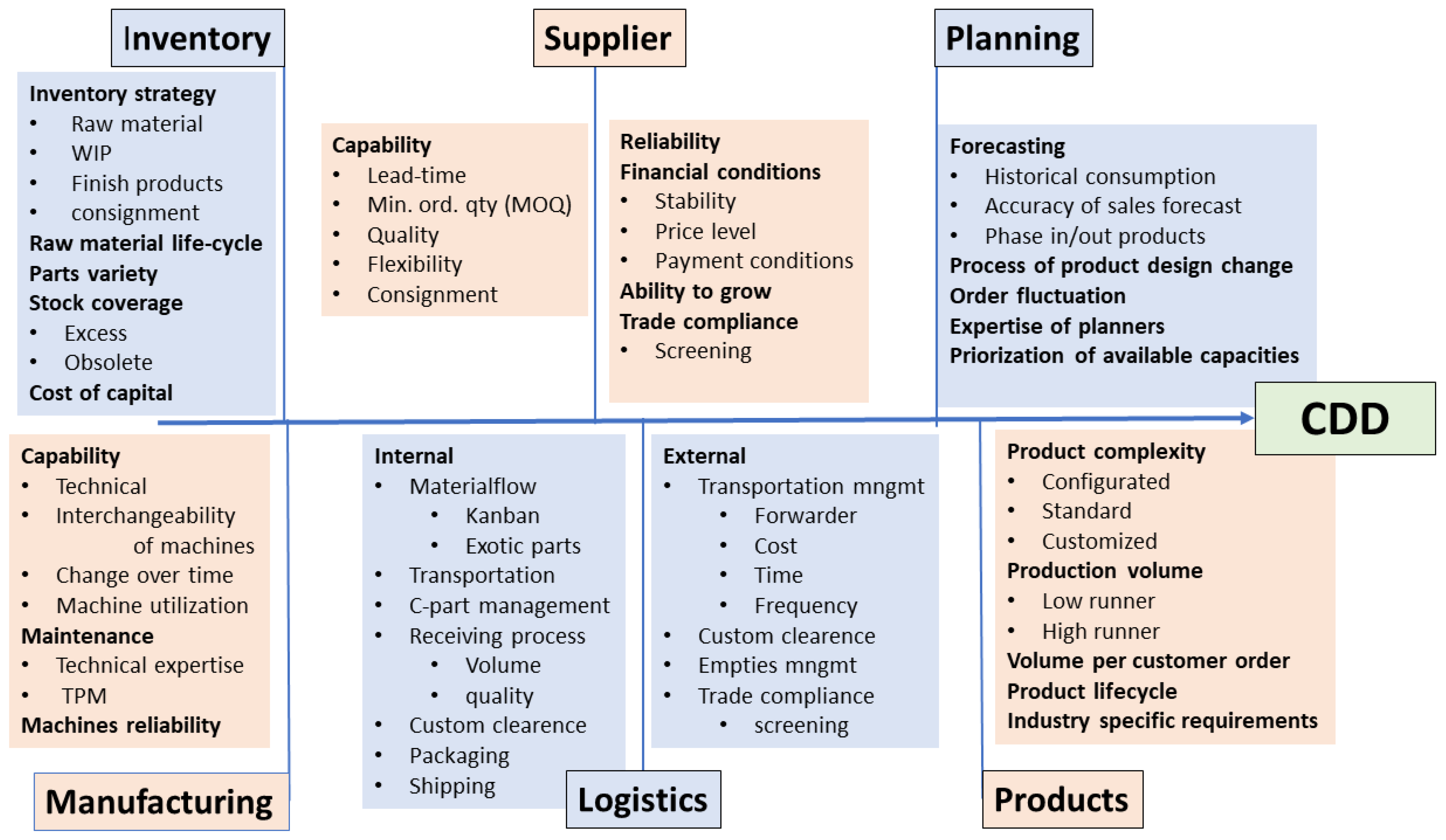
During a broad-sweeping, deep, and systematic analysis, we have identified and categorized all the main factors which are influencing the CDD delivery performance of our HMLV plant. The main categories are: (1) raw materials’ inventory level, (2) suppliers’ capability, (3) manufacturing capability, (4) logistics, (5) products’ complexity, and (6) quality of planning (see also Figure 7). A detailed description of these factors is as follows:

• Raw material inventory level: Raw material and subassembly availability define when production can be launched as early as possible. Increasing the raw material inventory level will certainly improve the delivery performance. However, with increasing the inventory level, the cost of capital will increase as well, and the overall profitability of a plant may decrease. A tradeoff between inventory (cost of capital) and CDD must be achieved on a plant level.
• Suppliers’ capability: Performance of suppliers is defined by several criteria, such as minimum order quantity (MOQ), quality of the delivered parts, delivery lead time, payment conditions, transportation cost, tooling cost and ownership, flexibility, and speed in reacting to the orders. Minimizing the number of suppliers can lead to high dependency with consequences that can carry high risks in the future.
• Manufacturing capability: In our case, manufacturing includes machining and assembly operations (manual, semiautomatic, and automatic). Manufacturing capabilities are impacted by the machines’ technical capability (age and condition), reliability, quality and efficiency of maintenance, level of total productive maintenance (TPM), and flexibility. Interchangeability of machines and equipment matters in case of breakdowns, and further important factors are skills of machine operators, programming capabilities of engineers and technicians, change over speed from one order to the other, utilization of machines, and the potential for upgrading existing machines or replacing them with a newer technology.
• Logistics: Here, we make distinction between external and internal logistics. External logistics is mainly related to transportation: the incoming and outgoing flow of materials. In internal logistics, the key factors are the processing of incoming materials (counting, quality checking, customs clearance, putting the parts on the shelf, just-in-time processing), raw or semi-finished material transportation to the manufacturing point (including Kanban box changes), and finished goods’ transportation from the machining/assembly area to the finished goods warehouse.
• Products’ complexity: In case of standard products, processes can be shorter and more predictable. When there are configurated and customized products, the delivery performance can differ significantly, even in cases when products are quite similar.
• Quality of sales, production, and supply planning: CDD depends very much on the quality of planning. Several factors determine the efficiency of planning: historical forecasting, lot-sizing, and scheduling policies, prioritization, skills of the planner, and reliability of available information coming from suppliers or production engineering.

5.3. Building and Validating a Simulation Model

After identifying the above factors, we analyzed their impact on delivery precision by discrete event simulation (DES). Note that DES was already routinely applied in our plant for validating and evaluating layouts. Here, a DES model of the mini-factory was validated and run in a number of scenarios characteristic to the variations of the above factors. The model of the existing mini-factory was built in the professional Plant Simulation software, with product-dependent stochastic operation and cycle times and sequence-dependent change-over times (characterized by product family, diameter, and stroke length). The layout and the corresponding operations of the mini-factory are shown in Figure 4 above.

Next, different simulation scenarios were generated by tweaking both external and internal factors. To keep experimentation manageable, from the factors discussed above, only the most characteristic ones were selected. Hence, typical external factors were the product code and the daily ordered volume, while internal factors were both structural (buffer sizes, operator, and machines’ availability) or behavioral, such as lot-sizing and sequencing policies. To execute the sensitivity analysis, the ultimate outputs of the simulation model were the completion dates of the orders and the total makespan of the daily production executed in three shifts.

In the next step, validation of the model was performed to demonstrate that this DES model can truly reproduce the operation of the original system. During the validation, the DES model was connected and fed with the real-life systems’ inputs, processing times, and buffer levels, thus forming a digital twin [22] of the mini-factory. Specifically, for a one-week period, we compared five points of the production flow’s real volume results with the simulated volume figures, and the duration of real operation times with the simulated duration times of operations (after cutting, cylinder and rod manufacturing, washing, and assembly). Whenever significant deviation was detected, we checked the root causes, and adjusted and fine-tuned the parameters of the simulation model. As an example, Figure 8 shows the distribution of the order lead times for different randomized simulation runs for the same scenario, compared to the measured data (black line). Note that at the time of the measurements, the mini-factory worked daily in two shifts only.

5.4. Rough-Cut Sensitivity Analysis

After the successful validation, the goal of the first series of simulation experiments was to analyze the sensitivity of CDD performance to the potential changes in the above key factors and select those ones where the chances of improvement are relatively high at the lowest possible costs. Hence, a rough-cut sensitivity analysis was performed by running the DES model of the mini-factory in a series of controlled experiments. Scenarios were systematically generated by tweaking the key external and internal factors. Specifically, we intended to find out which structural/statical or behavioral/dynamic factors have the highest and lowest impact on the output of the system determined by the confirmed delivery date performance, the makespan (MS) of production, as well as by the average net lead time (LT) of products. Compared to a baseline solution reflecting the actual situation, the following factors were changed between limits suggested by experienced planners (see Figure 4 and

Table 1. Factors systematically changed in the rough-cut sensitivity analysis (see also Figure 4 for color coding).

Operators’ Availability	Machine Availability		Lot Size	Sequencing	Buffer Size
100%	all	100%	basic	basic	100%
90%	DM2239	85%	50%	random diameter	200%
80%	DM2242	85%	20%	random family	50%
60%	DM2243	85%			25%
	HELLER	85%			1 piece
	TRAUB1600	85%
	TRAUB1657	85%
	KHZ PRESS	85%
	KHZ TEST	85%
	KPZ PRESS	85%
	KPZ TEST	85%

, where the baseline scenario is represented by the first row):

• Operators’ availability varied between 60% and 100%.
• Machines’ availability varied between 85% and 100%.
• Batch sizes were determined as originally requested in the order (lot-for-lot), 50% of order, and 25% of order.
• Sequencing was simulated with three different rules: (1) basic or original, (2) random, based on diameters, and (3) random, based on product family.
• Buffer sizes were set to 200%, 100%, 50%, 25%, 1 piece, and unlimited buffer sizes.
• Finally, daily demand variant patterns were generated from historical data.

By performing factorial experiments, i.e., systematically tweaking these parameters, we were interested in detecting their influence on the lead time of individual orders. Compared to the baseline case, ceteris paribus, always a single factor was changed, and particular instances were run ten times so as to account for the effect of random decisions within the model. Altogether, the sum of the net computational times took almost 24 h.

As a result of this rough-cut sensitivity analysis, we obtained a so-called tornado diagram which sorts the factors according to their maximal and minimal deviation from the baseline scenario (see Figure 9).

As the top of Figure 9 shows, the sizes of buffers between the operations have the highest influence on the lead time, and on the delivery performance, after all. The second highest influence comes from the availability of milling machines. Next, the sequencing and lot-sizing rules matter. Considerable (negative) deviations are shown in the bottom of Figure 9. Here, again, as in the top of Figure 9, buffer sizes, sequencing, and lot-sizing rules matter. However, machine capacities cannot be increased quickly and at relatively low expenses. Specifically, this option of improvement was not considered due to two reasons: (1) the urgently needed capacity cannot be assured in an urgent case, only at the price of overcapacities, and (2) additional investments would render this option significantly more expensive than any other ones. Hence, all in all, the targets of potential changes and further detailed investigations were: (1) the sizes of buffers, (2) the sequencing, as well as (3) the lot-sizing rules. Note that these three factors are easily controllable and changeable, at low (or no) cost.

6. Model- and Data-Driven Focused Analysis

In the course of the rough-cut sensitivity analysis, the DES model of the mini-factory was run only in some selected, albeit well-designed scenarios (as shown in Table 1). Here, having selected the key targets of potential changes, in this stage of the decision support workflow the goal was to use the model in massive series of experiments, to run it with demand patterns most characteristic to the HMLV load of the mini-factory. This came along with the resolution of two issues generic in manufacturing simulation:

• An input scenario represents a specific, individual case, and hence the output and the lessons learned can also hardly be generalized.
• Detailed simulation runs can be expensive in terms of computational times (see above).

We run the simulation model (1) with historical customer order (CO) data covering a longer, one-year long horizon, (2) but with selected daily demand patterns which faithfully also represented other days. Such a daily order set is given simply by the required products (stock keeping unit, SKU) and their quantities.

Given these generalized, and, at the same time, compressed daily demands, one can run detailed simulation experiments to select the best-fitting settings of internal factors referring to the structural (buffer sizes) and to the behavioral (sequencing and lot-sizing rules) parameters of the manufacturing system serving HMLV demand. Figure 10 below shows the experimental setup of this detailed analysis. Note that this is a combination of model- and data-driven analyses whose expected results are appropriate assignments of structural and behavioral parameters to particular daily demand patterns, i.e., we want to find the right buffers sizes, the right sequencing, and the right lot-sizing rules for the given daily CO mix which would minimize the orders’ lead time and the lead time variance. All in all, this would stabilize the CDD performance.

6.1. Learning over Daily Demand Mixes

As discussed above, the daily demand depends on the actual customer requirements, where the variation at the day-to-day level can be significant. However, even in such circumstances, in the long term and with sufficient experience, there can be found some characteristic demand patterns and fitting lot-sizing and sequencing rules which are well-applicable to solve the daily production scheduling problems. This is the task our production planners accomplish on a daily basis.

The daily demand varies regarding the product—characterized by product type, diameter, and stroke length—and product quantities. It can be represented by a vector, where each cell denotes the required daily amount of a particular product variant. Figure 11 below shows an example of the demand of three consecutive days, which for confidentiality reasons is color-coded (darker colors represent values below the annual average, lighter colors above average).

The crux of the problem is to find such days’ CO’s that are similar to several other daily order sets and together sufficiently represent the annual demand. To solve this, we decided to use machine learning. In this setting, two ways of machine learning could be used: supervised or unsupervised learning. In case of supervised learning, one should label every day, and the orders with different characteristics specific to that day. This approach would not make our problem easier, because we do not know how the planners characterized the days, what features they elaborated, and what labels they attached to the days. Indeed, it is their personal, tacit knowledge.

Hence, we decided to focus on the unsupervised (or self-supervised) learning approach. Specifically, the daily orders of the past year’s period were grouped into clusters by means of a k-means clustering method [25]. This method partitions a number of data points—in our case, the vectors representing daily demand—into k clusters in such a way that each vector belongs to a cluster, with the nearest mean (cluster centroid) serving as representative of the cluster. Hence, vectors with high similarities belong to the same cluster. In the end of the process, each cluster was represented by a single element—a typical daily demand vector—which was the closest to the geometrical mean (centroid) of the cluster. Distance and the nearest mean were defined by the Euclidean distance. Note that the number of clusters should be given as the input parameter for the algorithm. Based on expert judgment, we made clusters of the same annual demand mix with different k values.

The task was to define the minimum number of clusters which could represent the yearly order volume in such a way that their centroids could be used in the detailed simulation studies, and next, by our production planners in their everyday scheduling activity. In our records, we had 235 working days, with 235 vectors of daily customer orders. To find the correct grouping into clusters, we elaborated six experimental scenarios: the k-means clustering was run for 5, 10, 25, 50, 75, and 100 clusters. Figure 12 below shows the aggregated results, as a so-called heatmap. The columns (except the first six) are representing product variants, while rows represent the daily order quantities, which are color-coded (darker colors represent values below the annual average, lighter colors above average). High demands are depicted by high-intensity cells. The first six columns are for showing the results of the six ways of clustering. In Figure 12, daily orders are grouped according to the 25-means clustering. This can be seen in the zoomed-in sub-diagram on the right-hand side of the figure, which present fragments of two clusters. These two clusters have in common that demand for a single product variant, p, dominates all the others, while there are differences due to geometric variations and slight demand for another product variant, S.

6.2. Focused Simulations with Clustered Daily Demand

If we would have 235 clusters, then we would represent the reality that existed for that one-year period. If we would try to have only a few possible clusters to represent the annual orders, then the rough generalization would probably be very far from the reality. The real challenge was to find the minimum number of clusters which would help us to generalize and compress the demand, but at the same time, could still properly represent the performance measures close to that of the baseline on all 235 days.

Hence, once again, we performed factorial experiments for each daily demand representing the clusters by systematically changing the dynamic (sequencing and lot size rules) and the structural factors (buffer sizes). For each cluster and setting, we again run 10 simulations to neutralize the effects of randomized choices. We wanted to know which clustering still results in the same (or very similar) behavior of the manufacturing system compared to no clustering with respect to the main performance criteria. We aimed at finding the point where further generalization, i.e., compressing the annual demand into too few clusters, deteriorated far too much of the behavior (and consequently, the performance measures) of the mini-factory. Hence, our goal was to define the minimum number of clusters that could still properly represent the behavior system operating under the original demand.

6.3. Analyzing the Impact of Dynamic Changes

To determine the proper clustering to be used later by planners, further simulation experiments were run on the baseline dataset and the centroids by applying the combination of different sequencing and lot-sizing rules. Settings of the simulation model were determined by different lot-sizing (grouping and splitting) and sequencing rules. These rules were suggested by planners of the factory and by the literature [5,13,26,27]. The following options were investigated:

• Ordering was performed by: (1) A heuristics variant called the “base” rule, which was applied by our production planners in their everyday practice. Alternatively, (2) the “max” rule sorted products descending by their order quantities, and (3) an “oscillation” rule first took the highest and then the lowest order quantities, in an iterative manner.
• Sequencing was also determined by grouping rules which considered the products’ secondary attributes (such as diameter and length): (1) either products with the same diameters were put one after the other, (2) or diameters were not taken into consideration.
• Lot sizes and the sequence were also determined by lot-splitting rules: (1) The “local” rule split orders into product-specific lots. The sequencing of these split orders was not modified. (2) Alternatively, the “cycle” rule split orders at a predefined lot size value, and the first part of the order stayed in the sequence, while the second part was put at the end of the sequence. This part, if longer than the predefined lot size, was repeatedly cut by the “cycle” rule.

For example, consider three products, A, B, and C, with order quantities of 80, 120, and 40, respectively. Following the “base” rule, let the original sequence be A, B, and C. Assume that the predefined lot size is 40 for each product. Then, the “local” rule produces a sequence of A40, A40, B40, B40, B40, and C40, by keeping the original ordering of products intact. Instead, the “cycle” rule produces A40, B40, C40, A40, B40, and B40. In production, this would incur more setups, however, at the same time, it would open more opportunities for parallel processing.

The combination of the above rules resulted in 10 different sequencing methods, as presented in

Table 2. Rules defining the sequencing and lot-sizing of daily orders.

Ordering	Grouping	Lot-Splitting
base	{False}	{cycle, local}
max	{False, True}	{cycle, local}
oscillation (osc)	{False, True}	{cycle, local}

. The name of the actual rule is combined from its components, e.g., “base_False_cycle” stands for the basic heuristics, followed by no grouping and cyclic lot-splitting, while “oscillation_True_local” stands for an oscillating ordering, followed by grouping and local lot-splitting.

The original question was how well a centroid represented all other members of its cluster. Degree of fit was measured in terms of a critical KPI, namely the makespan. For each cluster member in the baseline dataset, under the same parameter settings, the value of its makespan was compared to the makespan of its representative (i.e., centroid). In particular, the performance metric for a given rule and clustering is the percentage of daily input mixes for which the application of the rule resulted in a makespan that remained below 105% of the best, minimal makespan for that specific input mix. The comparison of the different rules’ performance for each cluster is summarized in Figure 13. For each rule, one can compare its performance based on different clustering and on the baseline case (without clustering, pink column in each set). One can also qualitatively see that the performances of the same rules over the C5 and C10 clusters are rather different, while, as expected, fine-grained clusters such as C75 and C100 produce almost the same performance values as the original dataset. C25 or C50 suggest a compromise of representative power and compactness.

Performance differences between various clusters can also be assessed quantitatively, as shown in

Table 3. Performance comparison of sequencing over different clusters of the annual demand.

Dataset ID	C5	C10	C25	C50	C75	C100	Base
MAE.S	0.166	0.149	0.106	0.057	0.054	0.036	0.000
MS.S %	96.3	95.8	94.7	94.6	92.4	92.2	100.0

. Here, the MAE.S column shows, in terms of the Mean Absolute Error (MAE), the performance deviation between the baseline dataset and the other centroids with applying the best sequencing rules. The MS.S column displays the values of the makespan in percentage of the makespan of the baseline dataset for cases when the best-performing rule is applied. Since we were looking for the most compact clustering which still truly represented the baseline scenario in terms of performance criterion, we found that C25 was the appropriate cluster.

The results show that the effects of dynamic changes and the evaluation of different sequencing and lot-sizing rules can be successfully carried out on representative, but smaller, datasets created by unsupervised learning. It also became clear that it is worth adapting the sequencing and lot-sizing rules to the actual daily demand.

6.4. Analyzing the Impact of Structural Changes

While dynamic changes on the system’s operation can be performed easily and at no extra cost, even on a daily basis, structural changes—here, buffer size changes—require physical adjustments of the line and solid justification. In the simulation model, the buffer sizes could be increased by increasing the length of the conveyors in the cylinder manufacturing section of the mini-factory (see Figure 4). Over the course of the simulation experiments, the DES model was run with various conveyor length settings (always changing one at a time). The demand was taken, as above, from the baseline dataset as well as from the centroids of the various clusters. The basis of comparison was also the same, i.e., the aggregated performance measured by the makespan. Here, the specific performance measure was the percentage of cases when changing a given buffer resulted in the best makespan.

Column MAE.B of

Table 4. Aggregated performance comparison of buffer sizes over different clusters of the annual demand.

Dataset ID	C5	C10	C25	C50	C75	C100	Base
MAE.B	0.273	0.180	0.092	0.091	0.062	0.015	0.000

shows the Mean Absolute Error for the different clusters. As one can observe, when the generalization was using less clusters, the MAE.B values showed a higher deviation. C10′s deviation was almost double C25′s, while the errors for C25 and C50 were almost the same. Hence, C25 clustering again provides a “golden mean” between truthful representation and compactness. Note that C25 has similar values for buffer size changes as for dynamic changes, confirming its choice for representing the complete baseline dataset of orders.

All in all, running the above simulation experiments with the C25 clustering took ca. 10 times less computational effort than working with the baseline dataset, reducing a total computational time of ca. 9 h to below a tolerable 1 h.

6.5. Validation and Verification of the Results

The next step of the decision support workflow presented in Section 5 is the validation and verification of results. The main question of the former is whether after executing all the previous steps, could we meet the original engineering and managerial requirements? Could we devise a better, combined way of using both the models and data available in our cyber-physical production system? More specifically, could we make use of the DES model and the collected, historical data of orders in the interest of stabilizing CDD performance? The answer to these questions is affirmative, because the series of simulation experiments, combined with unsupervised learning over the dataset of historical orders, have shown the following:

• Rough-cut sensitivity analysis can highlight potential factors—both structural and behavioral—for change.
• Clustering can generate characteristic patterns of daily demand.
• Detailed simulation can help in finding the right structural settings (in our case, buffer sizes) and the context-dependent sequencing and lot-sizing rules which fit best to a given daily demand pattern.

We must emphasize that lessons drawn in every phase of the decision support workflow complied well with the so far implicit domain knowledge of our production planners. Hence, the next question was how can we verify that the suggested method really improves CDD performance? To answer this question, a new series of simulation experiments was designed and run, this time departing from the C25 clustering which offered the best compromise between representative power and efficiency. Conditions of the experiments were set as follows:

• The size of the most sensitive buffer was increased.
• The best-performing sequencing and lot-sizing rules were assigned to each member of the C25 cluster. Hence, these important decisions could be performed in a context-dependent manner.
• Each daily input mix was classified according to the C25 clustering, and the assigned sequencing and lot-sizing rules were applied.
• For each day, performance evaluation was calculated as the ratio of the makespan according to the new and the original protocols.
• Aggregated comparisons were performed in time windows of different lengths over a rolling horizon. Specifically, windows covering 1, 5, and 10 days were “pushed” through the whole 235-days-long horizon.

Results of these verification studies are summarized in

Table 5. Aggregated performance comparison of the new protocol based on the C25 clustering against the baseline dataset.

	Rolling Sum (1)	Rolling Sum (5)	Rolling Sum (10)
Mean	0.966	0.967	0.950
Std. dev.	0.512	0.233	0.170
25%	0.832	0.868	0.886
50%	0.933	0.907	0.905
75%	1.001	0.942	0.930

. Here, the columns present the aggregated results of experiments for each time window. Beyond the mean and the standard deviation of the ratios of the new and original makespans, Table 5 also shows the values for cases if 25%, 50%, and 75% of the data are around the mean. One can see that an absolute improvement cannot be warranted: for the one-day window, the value of the 75% neighborhood cell refers to this. However, improvement is consistent and significant as the length of the investigated time window is increasing, for every category (i.e., row in Table 5) of the comparison.

Hence, one can deduce that the C25 clustering and the corresponding situation-dependent sequencing and lot-sizing rules reliably improved the delivery performance of our HMLV manufacturing facility. With this solution, the everyday working methods of our production planners can be simplified and, at the same time, significantly improved.

6.6. Update and Maintenance of the Models

Customers’ behavior changes over time, due to global and local economic conditions and circumstances. See, for a positive instance, the economic boom around 2006, or the crises from 2008 or 2019–2020, caused by the COVID-19 pandemic. This phenomenon, which is especially characteristic in HMLV production, was tackled in our factory as well. The pre-COVID-19 period was different from the COVID-19 period, which was, again, different from the hopefully post-COVID-19 (or more precisely, 4th wave) period. During the first wave of COVID-19, one of the effects observed was that the number of orders from customers increased; however, the number of products per orders decreased in comparison to the previous period. Another change observed was the alteration of the product mix. Products with some special characteristics achieved a higher customer demand than other products from the same product family. This was clearly visible when the demand for mask manufacturing lines increased on the global level, or when many more breathing machine manufacturing lines and antiseptic as well as germicidal bottling lines were built to fulfill the sharply and continuously increasing demand.

Along with these market changes, the demand patterns shown in Figure 3 and Figure 11 were also changing. Hence, the new customer order patterns led us to obtain slightly different clusters. Based on our empirical observations, we needed to restart the whole workflow described in Section 5 periodically, within 3 to 6 months.

7. Overall Impacts of the Decision Support Workflow

The impact of the decision support mechanism presented above was also assessed by measurements both in the mini-factory and also in the broader context of our whole manufacturing facility. The main findings, related to the operation of the mini-factory, are the following:

• Daily inventories of parts and semi-finished products at the lines—the so-called Work-in-Process—decreased from an average level of 3000 pieces to 1000 pieces. Note that this did not render the increase of some in-line buffers unnecessary, since these served to accommodate extra demand not rare in HMLV production. Along with lower inventories, the lead time on these lines was reduced from 2.5–3 days to 1.6–2 days (see Section 4.2).
• In the meantime, one of the machining centers was replaced with a newer, more reliable machine. The rough-cut sensitivity analysis already suggested that such a change could have a substantial impact on delivery performance (see the tornado diagram in Figure 9), and this was what actually happened: according to our measurements, the delivery performance improved by 10%.

Our systematic efforts to find the root causes behind delivery performance issues and implementing changes to improve its reliability had beneficial factory-wide effects as well:

• Initiating a survey of key factors influencing CDD performance (see Section 5.1 and Figure 7) alone came with an overall improvement of the main KPIs in the range of 3–5%. This is because the survey made our decision-making mechanism more transparent, opened new channels of communication, and everyone in its place became more aware of the other colleagues’ ends and means when responding to challenges of HMLV production.
• Strikingly, the reliability of planning improved: in particular, the deviation between the planned and the realized lead times decreased by ca. 30%. This was partly due to assessing the key impact factors and making the planners conscious of them. Moreover, lessons learned in the mini-factory about the use of specific sequencing and lot-sizing policies could also be transferred to other segments of production (which were also managed by the same personnel).

For the time being, the biggest threats to stable delivery performance are unexpected machine breakdowns and, in the recent era of the COVID-19 pandemic, unprecedented material shortages. In these cases, re-balancing the production can only be achieved with overtime. Anticipating and preventing such situations would call for some novel forecasting, inventory handling, and supplier managing policies whose impact on delivery performance could also be assessed in the proposed framework.

8. Conclusions and Outlook

This paper discussed both the practical and theoretical aspects of the challenges in HMLV production and pointed to decision support as the main critical factor in providing the proper responses. In particular, it was explained that correct, and at the same time cost-efficient actions have to be found in a complex web of interrelated factors. Mathematical modeling, albeit desirable, can capture only a fragment of issues and their relations. However, in a competitive setting which is most characteristic to HMLV production, misses and mistakes are barely tolerated.

What remains at disposal to improve the quality and precision of decision-making under such circumstances are detailed simulation models and big datasets collected during the normal operation of a factory. Both are essential elements of modern cyber-physical production systems and readily available in factories which are equipped with quasi-standard Industry 4.0 tools and techniques.

This paper suggested a novel approach for the combined use of model- and data-driven analysis and decision-making, all in the ultimate service of improving the delivery performance of a HMLV facility. All of these new results were integrated into a workflow whose phases were presented in detail, while elaborating on a case study. Key findings were validated and verified by special series of simulation experiments. The everyday practice corroborated the results, even in the hard times of the COVID-19 pandemic [28].

Beyond the above improvements, the main benefits of the new approach are the following:

• Theoretical and practical analysis resulted in a comprehensive and structured set of factors, which essentially influence delivery performance in a factory. These findings have relevance well beyond the scope of HMLV production.
• Companies at the advanced level of Industry 4.0 maturity (which are not few, anymore) typically have some DES models of their production facilities and some consolidated datasets of their past demand. This paper presented a workflow for making new use of these digital assets. The rough-cut sensitivity analysis suggested here can help to set the focus on the most promising and cost-efficient factors to change.
• As it was shown, the need for massive simulation studies can be reduced by compressing demand data of past periods into a much smaller set of characteristic demand patterns. For this, an unsupervised learning method was suggested which retained the intrinsic structure of a complex HMLV demand mix.
• Simulation experiments made explicit the observation that the different demand patterns produced by learning can be best served by a fitting combination of sequencing and lot-splitting rules. Our day-to-day operation could be improved, accordingly, and we are convinced that the lesson is generic, applicable even beyond HMLV production.

Further improvement possibilities in managing our HMLV production system can be achieved through extending the simulation model into a continuously functioning digital twin. This would entail a nonstop back and forth communication between the simulation software and the real factory, opening new opportunities for a continuous correction capability, self-optimization, and self-learning.