2.2. Cole–Cole Model
The Cole–Cole model [
28] is widely used to describe the complex relative permittivity of biological tissues,
, and its equation is described as follows:
in which
N is the number of poles and thence the order of the model,
,
, is the permittivity at high frequencies,
is the static ionic conductivity, and
,
, and
are the static permittivity, the relaxation time constant, and the distribution parameter of the
n-th addend of the summation, respectively.
To take into account the conductivity of the material considered, the conductive term is added, obtaining the following expression:
where
is the static ionic conductivity.
Such a model incorporates the Debye model [
27]. Indeed, the main difference between the Debye and Cole–Cole models is that the latter includes exponent
, with
. When the exponent becomes smaller, the relaxation time distribution becomes broader, i.e., the transition between low- and high-frequency values becomes wider, and the peak on imaginary part of the spectrum also becomes wider.
The complexity of both the structure and composition of biological material is such that the dispersion region of each pole may be broadened by multiple contributions to it. The broadening of the dispersion could be empirically accounted for by using the Cole–Cole model [
29]. It is for that reason that the Cole–Cole model is expected to provide more accurate dielectric spectrum curve-fitting.
Nevertheless, we also consider the Debye model in our study as it is sometimes preferred for its simplicity [
4,
5,
7,
8,
9,
10] and easy implementation of computational EM methods, such as finite-difference time-domain FDTD (in the Cole–Cole model, the addition of the parameters
causes difficulties when transforming to the time domain because the fractional powers of frequency lead to fractional derivatives [
11]).
2.3. Curve Fitting Algorithms
Let
x be the vector of model parameters,
P its length, and
M the number of frequency points where the measures are taken. We define the data vector as follows (
stands for transposition):
in which the
mth component of the vector
y is the observed value
. Let the following:
be the model vector, here given by Equation (
4), with
being its estimation at
.
Solving the least squares problem means finding
such that the following is the case:
in which the function to minimize,
, is the
quadratic norm of the misfit
, which is a non-linear function such that
r with
.
Many studies in the literature have proposed metaheuristic algorithms for curve fitting, such as genetic algorithm, simulated annealing algorithm, particle swarm algorithm, hybrid variants, etc. [
11,
16,
30], because of their ability to deal with very large search spaces. However, they have non-negligible disadvantages: longer execution time, stochastic nature, and poor mathematical background. For these reasons, we preferred to focus on gradient-like algorithms by evaluating their performance in terms of what is considered their weakness: the choice of the starting point.
Thus, we address the non-linear fitting problem with two methods: the Levenberg–Marquardt Algorithm (LMA) and the Variable Projection Algorithm (VPA). The first is a classic algorithm already used in this context [
13,
14]; the other, to the best of our knowledge, is used for the first time for this problem.
2.3.1. Levenberg–Marquardt Algorithm
The Levenberg–Marquardt Algorithm [
21,
22] acts more similarly to a gradient-descent method when the parameters are far from their optimal value and acts more similarly to the Gauss–Newton method when the parameters are close to their optimal value [
31]. The equation for the step
h at the
kth iteration is as follows:
where
J is the Jacobian of
f, and
is the damping parameter. It controls both the magnitude and direction of
h, and it was chosen at each iteration. It can be shown [
22] that, at each iteration, Equation (
8) solves the minimization problem over a reduced set of admissible solutions, i.e., those that satisfy
, limiting the correction step within a region near
. The radius of the trust region
is a strictly decreasing function with
. When
, step
h is identical to that of the Gauss–Newton method and its magnitude assumes the maximum value. As
,
h tends towards the steepest descent direction, with the magnitude tending towards 0.
Based on the above, we infer the qualitative update rule for : if then the quadratic approximation works well and we can extend the trust region, i.e., it will be . Otherwise, the step is unsuccessful, and we reduce the trust region, i.e., it will be ; in this way, the next step tends toward the negative gradient method and a lower value of is more likely to be found.
The M
ATLAB implementation has been used, specifically the
lscurvefit function with the Levenberg–Marquardt option [
32].
2.3.2. Variable Projection Algorithm
The Variable Projection Algorithm [
23] is a method used to solve separable nonlinear least squares problems. The least squares problem is said to be separable when the model parameters can be separated into two sets of parameters: one that enter linearly into the model,
, and another set of parameters that enters the model non linearly,
, such that
. For each observation
of a separable nonlinear least squares problem, the model consists of the following linear combination:
where
is a nonlinear function that depends on nonlinear parameters. Functional
is written in terms of residual vector
r as follows:
in which the
j-th column of the matrix
is
. The linear parameters
c could be obtained from the knowledge of
a by solving the linear least squares problem:
which stands for the minimum-norm solution of the linear least squares problem for fixed
a, where
is the Moore–Penrose generalized inverse of
. By replacing this in Equation (
10), we obtain the Variable Projection functional:
The Variable Projection algorithm consists of two steps: first minimizing Equation (
12) with an iterative nonlinear method and then using the optimal value found for
a to solve for
c in Equation (
11) [
33]. The principal advantage is that the iterative nonlinear algorithm used to solve the first minimization problem works in a reduced space, and less initial guesses are necessary. A robust implementation in M
ATLAB, called
VARPRO [
34], has been adapted and used to deal with complex-value problems, choosing the Levenberg–Marquardt option for the solution of Equation (
12).
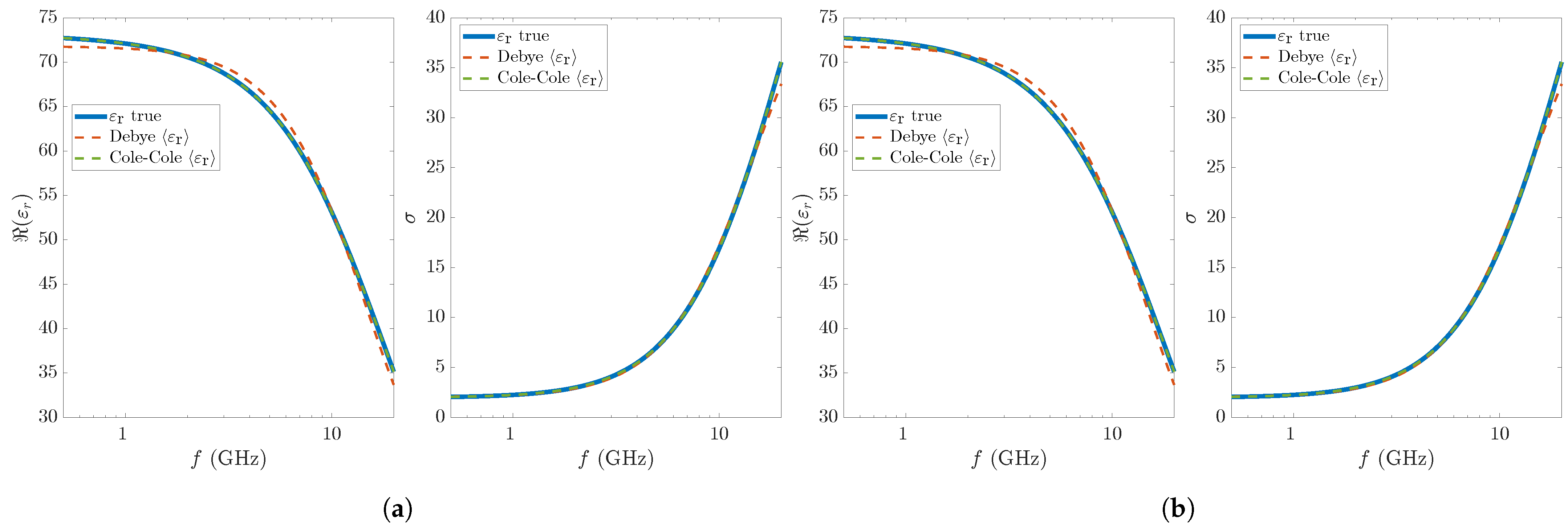
2.4. Numerical Simulations
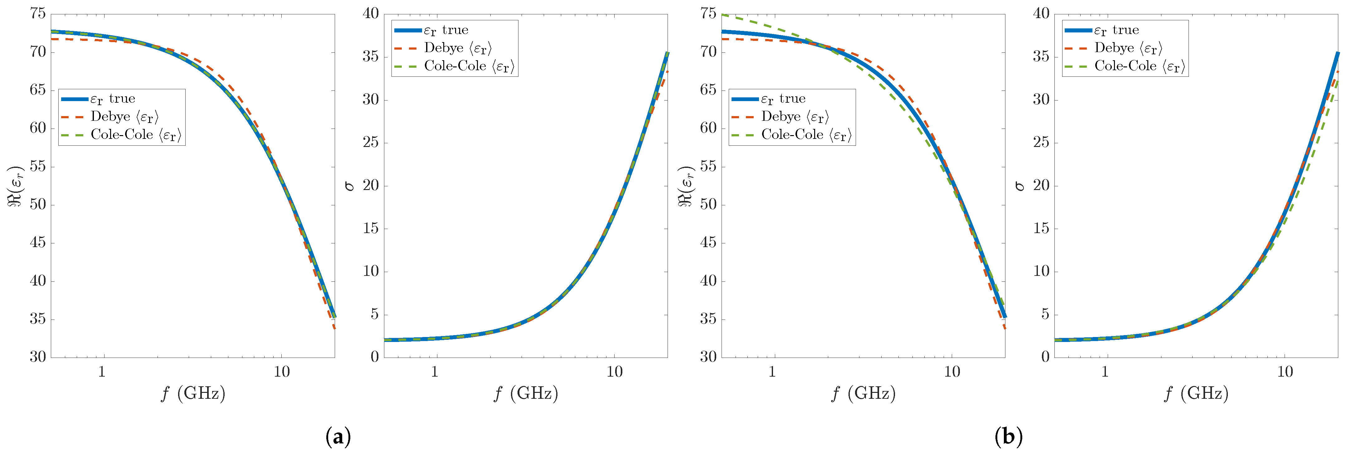
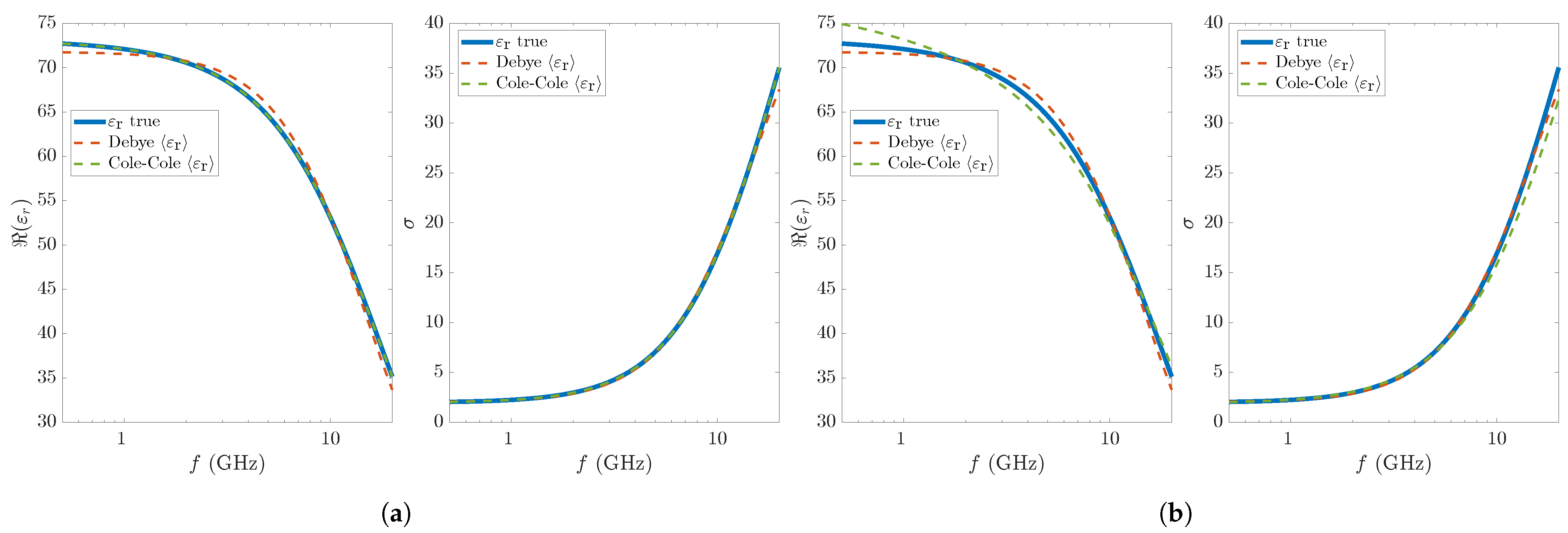
The generation of the synthetic complex relative permittivity of blood plasma relies on quadratic fits relative to glucose-dependent Cole–Cole parameters reported in [
24]; in particular, we consider two different concentrations, 100 mg/dL and 250 mg/dL, where the former is a normal value while the latter is typical of severe diabetes, respectively, in accordance with the diagnostic criteria in [
35]. The data vector consists of
points in the frequency range 500 MHz–20 GHz.
In gradient-like algorithms, the choice of the initial point is a crucial factor for the convergence of the procedure. For the single-pole model case, it is fairly easy to exploit the physical meaning of the parameters to infer an initial estimate. However, since the noise can invalidate the initial estimate, we propose to study the robustness of the two algorithms with respect to the initial point. To this end, a Monte Carlo analysis is performed, iteratively evaluating the deterministic algorithms using a set of uniformly distributed random initial points arranged in a 5D hypercube of the parameter space in order to statistically characterize the results. Each side of the hypercube represents an interval containing the range of variation of each parameter for the glucose concentrations considered.
We run simulations on a machine with Intel i9-10850K (10 physical cores), 32GB RAM, and Ubuntu 21.04, and we took advantage of the Parallel Computing Toolbox using the parfor loop for running the simulations.
The intervals for generating the random initial value for each parameter (of the Cole–Cole model) is chosen from the data tabulated in [
24]. In particular, the widths of these intervals are the same for each glucose concentration. We define three sets of intervals for the starting points with wider and wider intervals.
The first set, labeled as Set A, consists of the following intervals: for , for , for , for , and for .
The second set, labeled as Set B, consists of the following intervals: for , for , for , for , and for .
The third set, labeled as Set C, consists of the following intervals: for , for , for , for , and for .
These intervals are relatively large compared to the values taken from [
24] in order to test the two algorithms in sufficiently stressful situations. Obviously, it must be taken into account that VPA requires only the generation of
and
values for the Cole–Cole model and only of
values for the Debye model.
The algorithms are improved by introducing constraints on the parameters to be reconstructed. The required bounds are the following: for , for , for , for , and for .
For a quantitative evaluation of the performance of the two algorithms, we then define multiple figures of merit for statistically characterizing the results of the Monte Carlo analysis. For each parameter, mean and standard deviation are calculated over the entire set of reconstructions. Let the following:
be the vector of parameter estimates returned by the two algorithms at the
i-th simulation and let
denote one of its five elements. Moreover, let the following:
be the sample mean and standard deviation, respectively, calculated for each parameter.
To evaluate the accuracy of fitted curves, for each simulation, the root mean square relative error is calculated according to the following equation:
Mean and standard deviation of RMSRE over all simulations are finally calculated.


