Skin Cancer Disease Detection Using Transfer Learning Technique
Abstract
:1. Introduction
2. Related Work
3. Materials and Methods
3.1. Dataset
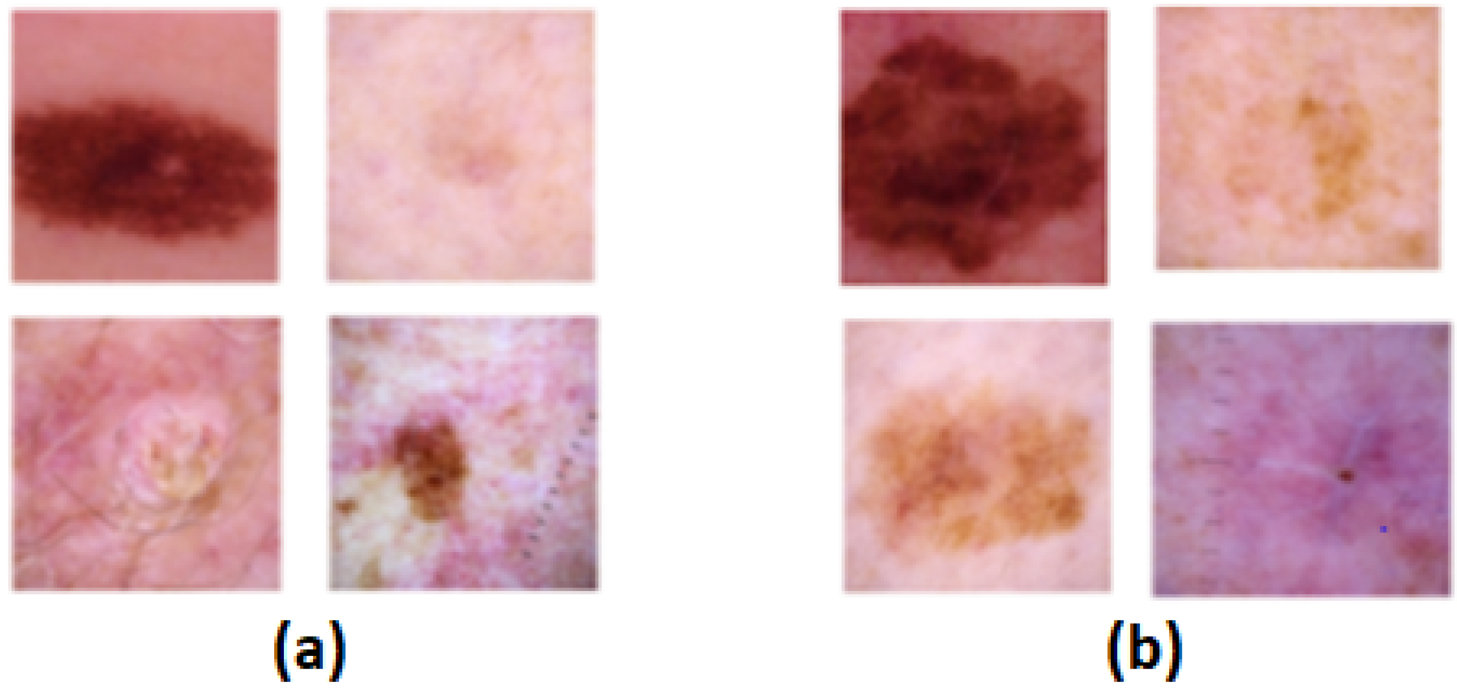
3.1.1. SIIM-ISIC 2020 Dataset
3.2. Image Pre-Processing
3.2.1. Image Resizing
3.2.2. Data Augmentation
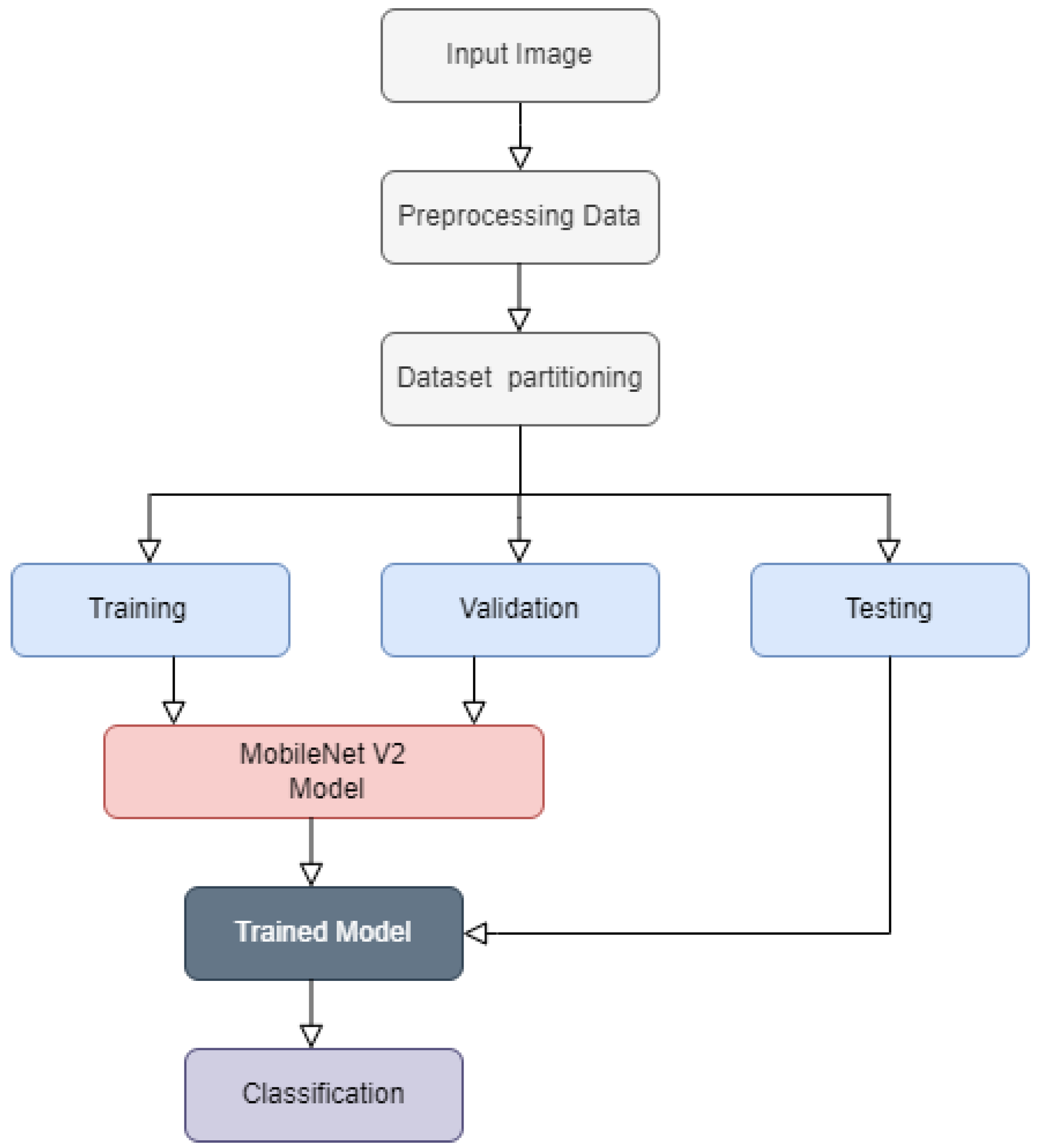
3.3. Training, Validation and Testing
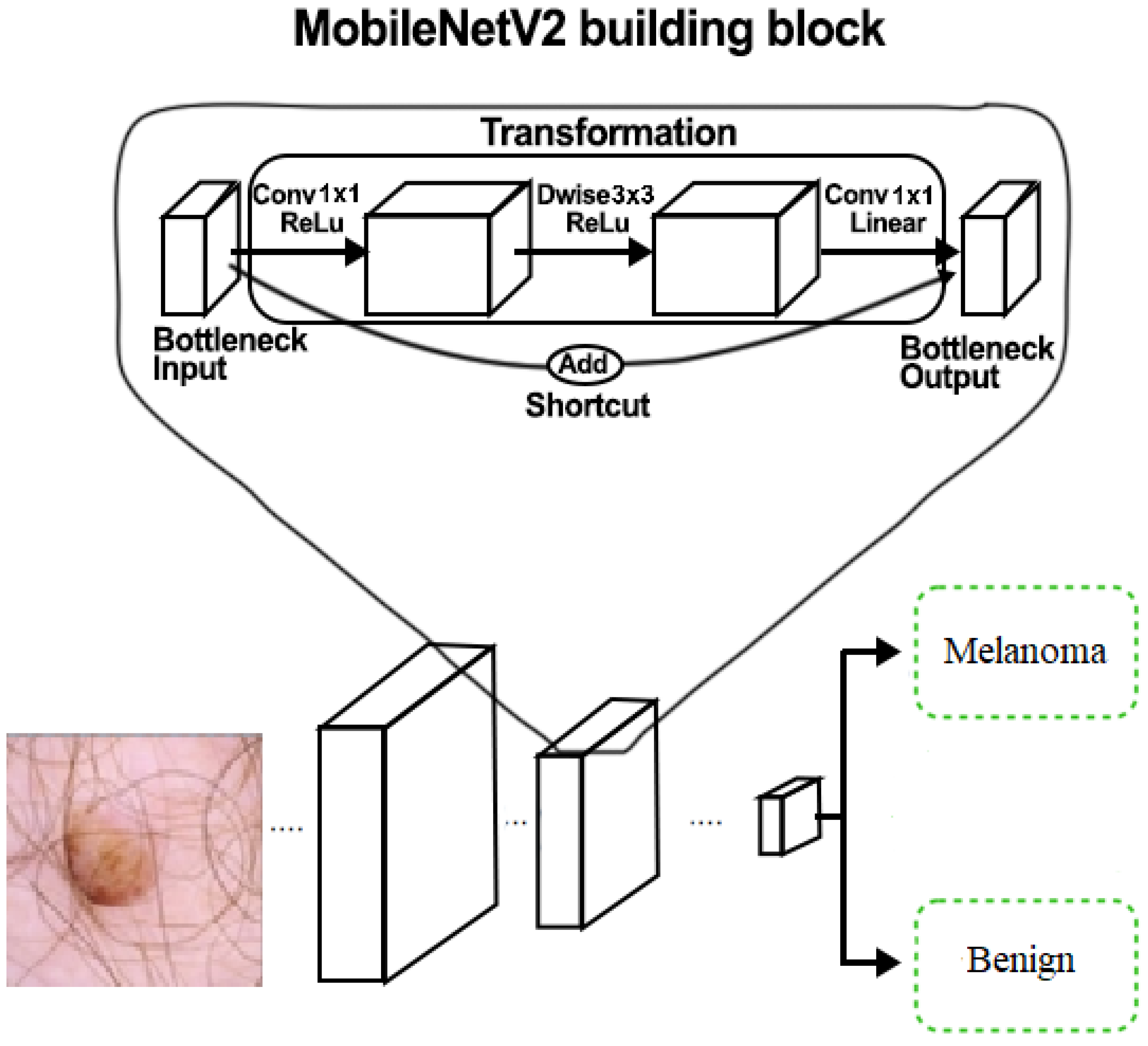
3.4. MobileNetV2 Architecture
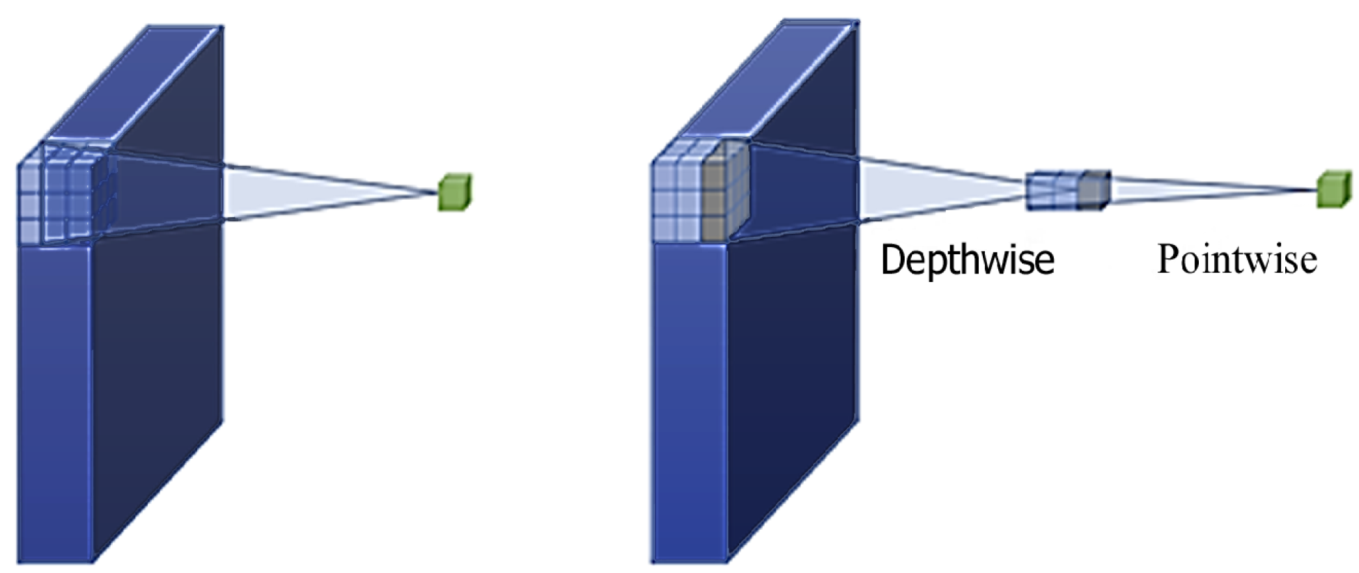
3.4.1. Depthwise Separable Convolutions
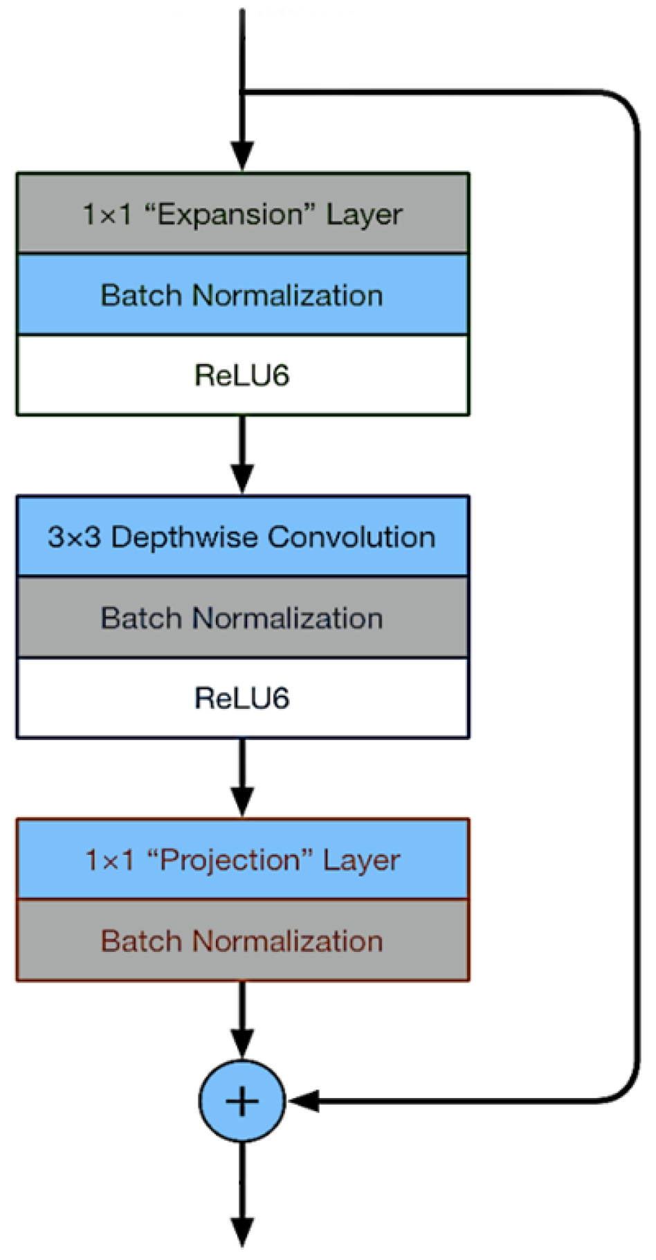
3.4.2. Linear Bottleneck and Inverted Residual
3.5. Evaluation Measures for Classification
3.5.1. Classification Accuracy
3.5.2. Precision
3.5.3. Recall
3.5.4. F1 Score
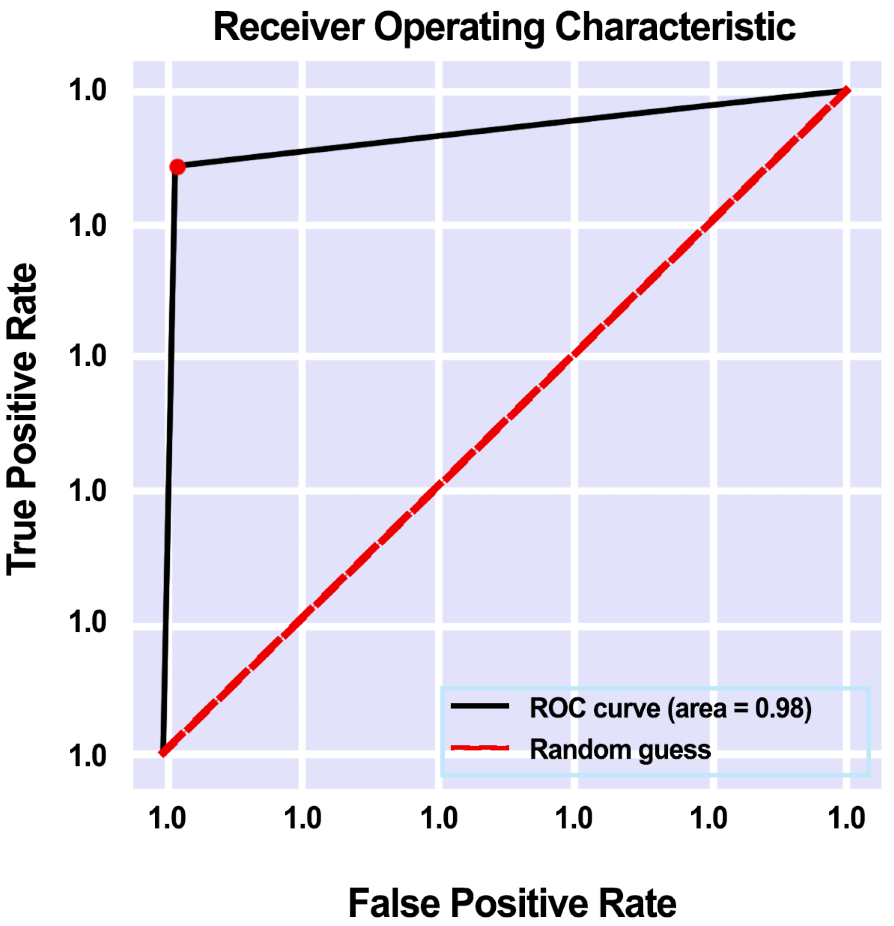
3.5.5. AUC Score and ROC Curve
4. Results and Discussion
- To differentiate the dermoscopic images into malignant or benign.
- Evaluated the performance of the presented MobileNetV2 model on the ISIC-2020 dataset by using various data augmentation techniques.
- The results were compared with state-of-the-art techniques.
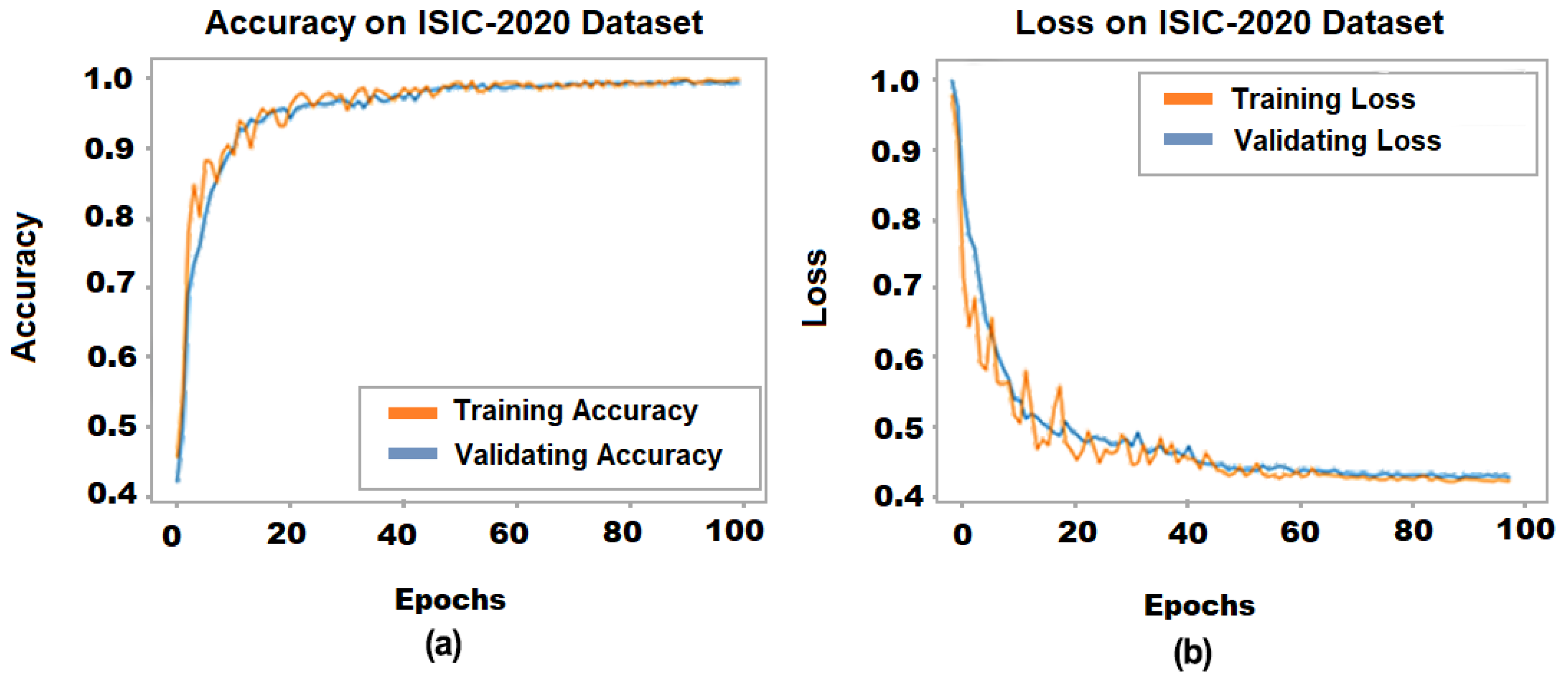
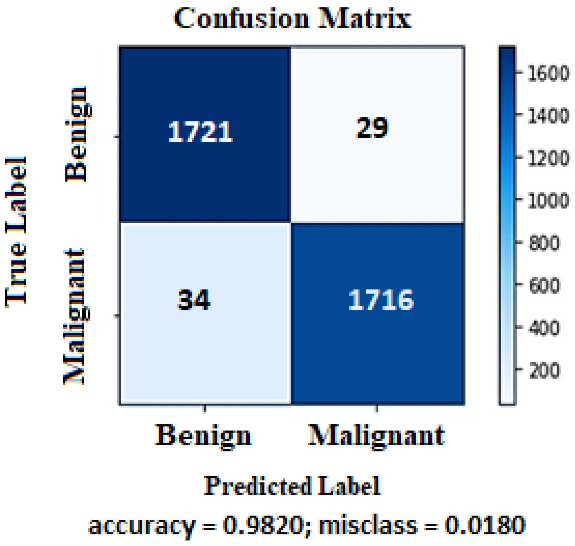
4.1. Proposed Model Performance on ISIC-2020 Dataset
4.2. Comparison with State-of-the-Art Methods
5. Conclusions and Future Work
Author Contributions
Funding
Institutional Review Board Statement
Informed Consent Statement
Data Availability Statement
Acknowledgments
Conflicts of Interest
References
- Factors, R. Basal and Squamous Cell Skin Cancer Causes, Risk Factors, and Prevention. 2019. Available online: https://www.cancer.org/content/dam/CRC/PDF/Public/8819.00.pdf (accessed on 2 March 2022).
- Gandhi, S.A.; Kampp, J. Skin cancer epidemiology, detection, and management. Med Clin. 2015, 99, 1323–1335. [Google Scholar] [CrossRef] [PubMed]
- Harrison, S.C.; Bergfeld, W.F. Ultraviolet light and skin cancer in athletes. Sport. Health 2009, 1, 335–340. [Google Scholar] [CrossRef] [PubMed] [Green Version]
- Skin Cancer. Available online: https://www.aad.org/media/stats-skin-cancer (accessed on 22 May 2022).
- Incidence estimate of nonmelanoma skin cancer (keratinocyte carcinomas) in the US population, 2012. JAMA Dermatol. 2015, 151, 1081–1086. [CrossRef] [PubMed]
- Whiteman, D.C.; Green, A.C.; Olsen, C.M. The growing burden of invasive melanoma: Projections of incidence rates and numbers of new cases in six susceptible populations through 2031. J. Investig. Dermatol. 2016, 136, 1161–1171. [Google Scholar] [CrossRef] [PubMed] [Green Version]
- Xie, F.; Fan, H.; Li, Y.; Jiang, Z.; Meng, R.; Bovik, A. Melanoma classification on dermoscopy images using a neural network ensemble model. IEEE Trans. Med. Imaging 2016, 36, 849–858. [Google Scholar] [CrossRef]
- Dalila, F.; Zohra, A.; Reda, K.; Hocine, C. Segmentation and classification of melanoma and benign skin lesions. Optik 2017, 140, 749–761. [Google Scholar] [CrossRef]
- Cancer Stat Facts: Melanoma of the Skin. Available online: https://seer.cancer.gov/statfacts/html/melan.html (accessed on 22 May 2022).
- Melanoma: Statistics. Available online: https://www.cancer.net/cancer-types/melanoma/statistics (accessed on 22 May 2022).
- Bomm, L.; Benez, M.D.V.; Maceira, J.M.P.; Succi, I.C.B.; Scotelaro, M.d.F.G. Biopsy guided by dermoscopy in cutaneous pigmented lesion-case report. An. Bras. Dermatol. 2013, 88, 125–127. [Google Scholar] [CrossRef] [Green Version]
- Kato, J.; Horimoto, K.; Sato, S.; Minowa, T.; Uhara, H. Dermoscopy of melanoma and non-melanoma skin cancers. Front. Med. 2019, 6, 180. [Google Scholar] [CrossRef] [Green Version]
- Gershenwald, J.E.; Scolyer, R.A.; Hess, K.R.; Sondak, V.K.; Long, G.V.; Ross, M.I.; Lazar, A.J.; Faries, M.B.; Kirkwood, J.M.; McArthur, G.A.; et al. Melanoma staging: Evidence-based changes in the American Joint Committee on Cancer eighth edition cancer staging manual. CA Cancer J. Clin. 2017, 67, 472–492. [Google Scholar] [CrossRef] [Green Version]
- Ibrahim, H.; El-Taieb, M.; Ahmed, A.; Hamada, R.; Nada, E. Dermoscopy versus skin biopsy in diagnosis of suspicious skin lesions. Al-Azhar Assiut Med. J. 2017, 15, 203. [Google Scholar] [CrossRef]
- Bajwa, M.N.; Muta, K.; Malik, M.I.; Siddiqui, S.A.; Braun, S.A.; Homey, B.; Dengel, A.; Ahmed, S. Computer-aided diagnosis of skin diseases using deep neural networks. Appl. Sci. 2020, 10, 2488. [Google Scholar] [CrossRef] [Green Version]
- Carli, P.; Quercioli, E.; Sestini, S.; Stante, M.; Ricci, L.; Brunasso, G.; De Giorgi, V. Pattern analysis, not simplified algorithms, is the most reliable method for teaching dermoscopy for melanoma diagnosis to residents in dermatology. Br. J. Dermatol. 2003, 148, 981–984. [Google Scholar] [CrossRef] [PubMed]
- Carrera, C.; Marchetti, M.A.; Dusza, S.W.; Argenziano, G.; Braun, R.P.; Halpern, A.C.; Jaimes, N.; Kittler, H.J.; Malvehy, J.; Menzies, S.W.; et al. Validity and reliability of dermoscopic criteria used to differentiate nevi from melanoma: A web-based international dermoscopy society study. JAMA Dermatol. 2016, 152, 798–806. [Google Scholar] [CrossRef] [PubMed] [Green Version]
- Gutman, D.; Codella, N.C.; Celebi, E.; Helba, B.; Marchetti, M.; Mishra, N.; Halpern, A. Skin lesion analysis toward melanoma detection: A challenge at the international symposium on biomedical imaging (ISBI) 2016, hosted by the international skin imaging collaboration (ISIC). arXiv 2016, arXiv:1605.01397. [Google Scholar]
- Binder, M.; Kittler, H.; Seeber, A.; Steiner, A.; Pehamberger, H.; Wolff, K. Epiluminescence microscopy-based classification of pigmented skin lesions using computerized image analysis and an artificial neural network. Melanoma Res. 1998, 8, 261–266. [Google Scholar] [CrossRef]
- Burroni, M.; Corona, R.; Dell’Eva, G.; Sera, F.; Bono, R.; Puddu, P.; Perotti, R.; Nobile, F.; Andreassi, L.; Rubegni, P. Melanoma computer-aided diagnosis: Reliability and feasibility study. Clin. Cancer Res. 2004, 10, 1881–1886. [Google Scholar] [CrossRef] [Green Version]
- Nath, R.P.; Balaji, V.N. Artificial intelligence in power systems. IOSR J. Comput. Eng. (IOSR-JCE) 2014, e-ISSN, 2278-0661. [Google Scholar]
- Sivadasan, B. Application of artificial intelligence in electrical engineering. In Proceedings of the National Conference on Emerging Research Trend in Electrical and Electronics Engineering (ERTEE 2018), Kalady, Kerala, 25 March 2018. [Google Scholar]
- Xu, Y.; Ahokangas, P.; Louis, J.N.; Pongrácz, E. Electricity market empowered by artificial intelligence: A platform approach. Energies 2019, 12, 4128. [Google Scholar] [CrossRef] [Green Version]
- Kourou, K.; Exarchos, T.P.; Exarchos, K.P.; Karamouzis, M.V.; Fotiadis, D.I. Machine learning applications in cancer prognosis and prediction. Comput. Struct. Biotechnol. J. 2015, 13, 8–17. [Google Scholar] [CrossRef] [Green Version]
- Cruz, J.A.; Wishart, D.S. Applications of machine learning in cancer prediction and prognosis. Cancer Inform. 2006, 2, 117693510600200030. [Google Scholar] [CrossRef]
- Sohail, M.; Ali, G.; Rashid, J.; Ahmad, I.; Almotiri, S.H.; AlGhamdi, M.A.; Nagra, A.A.; Masood, K. Racial Identity-Aware Facial Expression Recognition Using Deep Convolutional Neural Networks. Appl. Sci. 2021, 12, 88. [Google Scholar] [CrossRef]
- Rashid, J.; Khan, I.; Ali, G.; Almotiri, S.H.; AlGhamdi, M.A.; Masood, K. Multi-Level Deep Learning Model for Potato Leaf Disease Recognition. Electronics 2021, 10, 2064. [Google Scholar] [CrossRef]
- Dargan, S.; Kumar, M.; Ayyagari, M.R.; Kumar, G. A survey of deep learning and its applications: A new paradigm to machine learning. Arch. Comput. Methods Eng. 2020, 27, 1071–1092. [Google Scholar] [CrossRef]
- Hordri, N.F.; Yuhaniz, S.S.; Shamsuddin, S.M. Deep learning and its applications: A review. In Proceedings of the Conference on Postgraduate Annual Research on Informatics Seminar, Kuala Lumpur, Malaysia, 12 September 2016. [Google Scholar]
- Najafabadi, M.M.; Villanustre, F.; Khoshgoftaar, T.M.; Seliya, N.; Wald, R.; Muharemagic, E. Deep learning applications and challenges in big data analytics. J. Big Data 2015, 2, 1–21. [Google Scholar] [CrossRef] [Green Version]
- LeCun, Y.; Bengio, Y.; Hinton, G. Deep learning. Nature 2015, 521, 436–444. [Google Scholar] [CrossRef] [PubMed]
- Brinker, T.J.; Hekler, A.; Utikal, J.S.; Grabe, N.; Schadendorf, D.; Klode, J.; Berking, C.; Steeb, T.; Enk, A.H.; Von Kalle, C. Skin cancer classification using convolutional neural networks: Systematic review. J. Med. Internet Res. 2018, 20, e11936. [Google Scholar] [CrossRef]
- Fujisawa, Y.; Inoue, S.; Nakamura, Y. The possibility of deep learning-based, computer-aided skin tumor classifiers. Front. Med. 2019, 6, 191. [Google Scholar] [CrossRef] [Green Version]
- Litjens, G.; Kooi, T.; Bejnordi, B.E.; Setio, A.A.A.; Ciompi, F.; Ghafoorian, M.; Van Der Laak, J.A.; Van Ginneken, B.; Sánchez, C.I. A survey on deep learning in medical image analysis. Med. Image Anal. 2017, 42, 60–88. [Google Scholar] [CrossRef] [Green Version]
- He, K.; Zhang, X.; Ren, S.; Sun, J. Deep residual learning for image recognition. In Proceedings of the IEEE Conference on Computer Vision and Pattern Recognition, Las Vegas, NV, USA, 27–30 June 2016; pp. 770–778. [Google Scholar]
- Kong, B.; Sun, S.; Wang, X.; Song, Q.; Zhang, S. Invasive cancer detection utilizing compressed convolutional neural network and transfer learning. In Proceedings of the International Conference on Medical Image Computing and Computer-Assisted Intervention, Granada, Spain, 16–20 September 2018; Springer: Berlin/Heidelberg, Germany, 2018; pp. 156–164. [Google Scholar]
- Wu, S.; Gao, Z.; Liu, Z.; Luo, J.; Zhang, H.; Li, S. Direct reconstruction of ultrasound elastography using an end-to-end deep neural network. In Proceedings of the International Conference on Medical Image Computing and Computer-Assisted Intervention, Granada, Spain, 16–20 September 2018; Springer: Berlin/Heidelberg, Germany, 2018; pp. 374–382. [Google Scholar]
- Codella, N.; Cai, J.; Abedini, M.; Garnavi, R.; Halpern, A.; Smith, J.R. Deep learning, sparse coding, and SVM for melanoma recognition in dermoscopy images. In Proceedings of the International Workshop on Machine Learning in Medical Imaging, Lille, France, 11 July 2015; Springer: Berlin/Heidelberg, Germany, 2015; pp. 118–126. [Google Scholar]
- Haenssle, H.A.; Fink, C.; Schneiderbauer, R.; Toberer, F.; Buhl, T.; Blum, A.; Kalloo, A.; Hassen, A.B.H.; Thomas, L.; Enk, A.; et al. Man against machine: Diagnostic performance of a deep learning convolutional neural network for dermoscopic melanoma recognition in comparison to 58 dermatologists. Ann. Oncol. 2018, 29, 1836–1842. [Google Scholar] [CrossRef]
- Kawahara, J.; Hamarneh, G. Multi-resolution-tract CNN with hybrid pretrained and skin-lesion trained layers. In Proceedings of the International Workshop on Machine Learning in Medical Imaging, Athens, Greece, 17 October 2016; Springer: Berlin/Heidelberg, Germany, 2016; pp. 164–171. [Google Scholar]
- Li, Y.; Shen, L. Skin lesion analysis towards melanoma detection using deep learning network. Sensors 2018, 18, 556. [Google Scholar] [CrossRef] [Green Version]
- Menegola, A.; Fornaciali, M.; Pires, R.; Bittencourt, F.V.; Avila, S.; Valle, E. Knowledge transfer for melanoma screening with deep learning. In Proceedings of the 2017 IEEE 14th international symposium on biomedical imaging (ISBI 2017), Melbourne, Australia, 18–21 April 2017; pp. 297–300. [Google Scholar]
- Giotis, I.; Molders, N.; Land, S.; Biehl, M.; Jonkman, M.F.; Petkov, N. MED-NODE: A computer-assisted melanoma diagnosis system using non-dermoscopic images. Expert Syst. Appl. 2015, 42, 6578–6585. [Google Scholar] [CrossRef]
- Lynn, N.C.; War, N. Melanoma classification on dermoscopy skin images using bag tree ensemble classifier. In Proceedings of the 2019 International Conference on Advanced Information Technologies (ICAIT), Yangon, Myanmar, 6–7 November 2019; pp. 120–125. [Google Scholar]
- Mukherjee, S.; Adhikari, A.; Roy, M. Melanoma identification using MLP with parameter selected by metaheuristic algorithms. In Intelligent Innovations in Multimedia Data Engineering and Management; IGI Global: Hershey, PA, USA, 2019; pp. 241–268. [Google Scholar]
- Khan, M.Q.; Hussain, A.; Rehman, S.U.; Khan, U.; Maqsood, M.; Mehmood, K.; Khan, M.A. Classification of melanoma and nevus in digital images for diagnosis of skin cancer. IEEE Access 2019, 7, 90132–90144. [Google Scholar] [CrossRef]
- Filali, Y.; El Khoukhi, H.; Sabri, M.A.; Aarab, A. Efficient fusion of handcrafted and pre-trained CNNs features to classify melanoma skin cancer. Multimed. Tools Appl. 2020, 79, 31219–31238. [Google Scholar] [CrossRef]
- Hu, K.; Niu, X.; Liu, S.; Zhang, Y.; Cao, C.; Xiao, F.; Yang, W.; Gao, X. Classification of melanoma based on feature similarity measurement for codebook learning in the bag-of-features model. Biomed. Signal Process. Control 2019, 51, 200–209. [Google Scholar] [CrossRef]
- Abbas, Q.; Celebi, M.E. DermoDeep-A classification of melanoma-nevus skin lesions using multi-feature fusion of visual features and deep neural network. Multimed. Tools Appl. 2019, 78, 23559–23580. [Google Scholar] [CrossRef]
- Almansour, E.; Jaffar, M.A. Classification of Dermoscopic skin cancer images using color and hybrid texture features. IJCSNS Int. J. Comput. Sci. Netw. Secur. 2016, 16, 135–139. [Google Scholar]
- Pham, T.C.; Luong, C.M.; Visani, M.; Hoang, V.D. Deep CNN and data augmentation for skin lesion classification. In Asian Conference on Intelligent Information and Database Systems; Springer: Berlin/Heidelberg, Germany, 2018; pp. 573–582. [Google Scholar]
- Yu, L.; Chen, H.; Dou, Q.; Qin, J.; Heng, P.A. Automated melanoma recognition in dermoscopy images via very deep residual networks. IEEE Trans. Med. Imaging 2016, 36, 994–1004. [Google Scholar] [CrossRef]
- Yu, Z.; Jiang, X.; Zhou, F.; Qin, J.; Ni, D.; Chen, S.; Lei, B.; Wang, T. Melanoma recognition in dermoscopy images via aggregated deep convolutional features. IEEE Trans. Biomed. Eng. 2018, 66, 1006–1016. [Google Scholar] [CrossRef]
- Rokhana, R.; Herulambang, W.; Indraswari, R. Deep convolutional neural network for melanoma image classification. In Proceedings of the 2020 International Electronics Symposium (IES), Marrakech, Morocco, 24–26 March 2020; pp. 481–486. [Google Scholar]
- Liberman, G.; Acevedo, D.; Mejail, M. Classification of melanoma images with fisher vectors and deep learning. In Iberoamerican Congress on Pattern Recognition; Springer: Berlin/Heidelberg, Germany, 2018; pp. 732–739. [Google Scholar]
- Zhou, Q.; Shi, Y.; Xu, Z.; Qu, R.; Xu, G. Classifying melanoma skin lesions using convolutional spiking neural networks with unsupervised stdp learning rule. IEEE Access 2020, 8, 101309–101319. [Google Scholar] [CrossRef]
- Hosny, K.M.; Kassem, M.A.; Foaud, M.M. Skin melanoma classification using ROI and data augmentation with deep convolutional neural networks. Multimed. Tools Appl. 2020, 79, 24029–24055. [Google Scholar] [CrossRef]
- Mukherjee, S.; Adhikari, A.; Roy, M. Malignant melanoma classification using cross-platform dataset with deep learning CNN architecture. In Recent Trends in Signal and Image Processing; Springer: Berlin/Heidelberg, Germany, 2019; pp. 31–41. [Google Scholar]
- Esteva, A.; Kuprel, B.; Thrun, S. Deep Networks for Early Stage Skin Disease and Skin Cancer Classification; Stanford University: Stanford, CA, USA, 2015. [Google Scholar]
- Çakmak, M.; Tenekecı, M.E. Melanoma detection from dermoscopy images using Nasnet Mobile with Transfer Learning. In Proceedings of the 2021 29th Signal Processing and Communications Applications Conference (SIU), Istanbul, Turkey, 9–11 June 2021; pp. 1–4. [Google Scholar]
- Brinker, T.J.; Hekler, A.; Enk, A.H.; Berking, C.; Haferkamp, S.; Hauschild, A.; Weichenthal, M.; Klode, J.; Schadendorf, D.; Holland-Letz, T.; et al. Deep neural networks are superior to dermatologists in melanoma image classification. Eur. J. Cancer 2019, 119, 11–17. [Google Scholar] [CrossRef] [Green Version]
- Han, S.S.; Kim, M.S.; Lim, W.; Park, G.H.; Park, I.; Chang, S.E. Classification of the clinical images for benign and malignant cutaneous tumors using a deep learning algorithm. J. Investig. Dermatol. 2018, 138, 1529–1538. [Google Scholar] [CrossRef] [PubMed] [Green Version]
- Hosny, K.M.; Kassem, M.A.; Foaud, M.M. Classification of skin lesions using transfer learning and augmentation with Alex-net. PLoS ONE 2019, 14, e0217293. [Google Scholar] [CrossRef] [PubMed] [Green Version]
- Esteva, A.; Kuprel, B.; Novoa, R.A.; Ko, J.; Swetter, S.M.; Blau, H.M.; Thrun, S. Dermatologist-level classification of skin cancer with deep neural networks. Nature 2017, 542, 115–118. [Google Scholar] [CrossRef] [PubMed]
- Shaikhina, T.; Lowe, D.; Daga, S.; Briggs, D.; Higgins, R.; Khovanova, N. Machine learning for predictive modelling based on small data in biomedical engineering. IFAC-PapersOnLine 2015, 48, 469–474. [Google Scholar] [CrossRef]
- Attaran, M.; Deb, P. Machine learning: The new’big thing’for competitive advantage. Int. J. Knowl. Eng. Data Min. 2018, 5, 277–305. [Google Scholar] [CrossRef]
- Reichstein, M.; Camps-Valls, G.; Stevens, B.; Jung, M.; Denzler, J.; Carvalhais, N. Deep learning and process understanding for data-driven Earth system science. Nature 2019, 566, 195–204. [Google Scholar] [CrossRef]
- Sarvepalli, S.K. Deep Learning in Neural Networks: The Science Behind an Artificial Brain; Liverpool Hope University: Liverpool, UK, 2015. [Google Scholar]
- The ISIC 2020 Challenge Dataset. Available online: https://challenge2020.isic-archive.com/ (accessed on 5 March 2022).
- The ISIC 2019 Challenge Dataset. Available online: https://challenge2019.isic-archive.com/ (accessed on 5 March 2022).
- Sandler, M.; Howard, A.; Zhu, M.; Zhmoginov, A.; Chen, L.C. Mobilenetv2: Inverted residuals and linear bottlenecks. In Proceedings of the IEEE Conference on Computer Vision and Pattern Recognition, Salt Lake City, UT, USA, 18–23 June 2018; pp. 4510–4520. [Google Scholar]
- Zhang, X.; Zhou, X.; Lin, M.; Sun, J. Shufflenet: An extremely efficient convolutional neural network for mobile devices. In Proceedings of the IEEE conference on computer vision and pattern recognition, Salt Lake City, UT, USA, 18–23 June 2018; pp. 6848–6856. [Google Scholar]
- Chollet, F. Xception: Deep learning with depthwise separable convolutions. In Proceedings of the IEEE Conference on Computer Vision and Pattern Recognition, Honolulu, HI, USA, 21–26 July 2017; pp. 1251–1258. [Google Scholar]
- Howard, A.G.; Zhu, M.; Chen, B.; Kalenichenko, D.; Wang, W.; Weyand, T.; Andreetto, M.; Adam, H. Mobilenets: Efficient convolutional neural networks for mobile vision applications. arXiv 2017, arXiv:1704.04861. [Google Scholar]
- Mijwil, M.M. Skin cancer disease images classification using deep learning solutions Multimedia Tools and Applications. Multimed. Tools Appl. 2021, 80, 26255–26271. [Google Scholar] [CrossRef]
| Reference | Methodology | Disease | Dataset | Accuracy |
|---|---|---|---|---|
| [60] | Nasnet Mobile with | Melanoma | HAM10000 skin | 97.90% |
| Transfer Learning | lesion dataset | |||
| [46] | Support Vector Machine | Melanoma, Nevus | DERMIS dataset | 96.0% |
| (SVM) | ||||
| [53] | DCNN-FV | Melanoma, | ISBI 2016 | 86.54% |
| Non-Melanoma | challenge | |||
| [54] | Deep Convolutional | Benign, | ISIC Archive | 84.76% |
| Neural Network (CNN) | Malignant, Melanoma | Repository | ||
| [47] | SVM | Melanoma, | Ph2 & ISIC | Ph2 98%, |
| Non-Melanoma | Challenge | ISIC 87.8% | ||
| [7] | Ensemble Model | Malignant, | Xanthous Race (XR), | XR (94.14%), |
| Benign | Caucasian Race (CR) | CR (91.11%) | ||
| [48] | FSM & SVM | Malignant, | Ph2 | 91.90% |
| Benign | ||||
| [49] | DCNN | Melanoma, | Self Contained | 96% |
| Nevi | 2800 Images | |||
| [8] | ANN | Malignant, | Self Contained | 93.6% |
| Benign | 172 Images | |||
| [61] | ResNet-50 | Melanoma, | Self Contained | Sensitivity (82.3%), |
| Nevi | 4204 Images | Specificity (77.9%) | ||
| [55] | Ensemble Model | Melanoma, | ISIC | Avg Precision |
| Non-Melanoma | (98.0%) | |||
| [56] | STDP based | Malignant, | ISIC 2018 | 87.7% |
| Spiking NN | Melanoma, | |||
| Benign, Nevi | ||||
| [57] | DCNN | Melanocytic, | MED-NODE | MED-NODE |
| Non-melanocytic | DermIS & DermQuest | (99.29%), | ||
| (D&D), | D&D(99.15%), | |||
| ISIC-2017 | ISIC(98.14%) | |||
| [58] | CNN based | Melanoma, | Dermofit, | Dermofit |
| CMLD model | Benign | MED-NODE | (90.58%), | |
| MED-NODE | ||||
| (90.14%) |
| Class Labels | Training | Validation | Testing |
|---|---|---|---|
| Melanoma | 8170 | 1750 | 1750 |
| Benign | 8170 | 1750 | 1750 |
| Total | 16,340 | 3500 | 3500 |
| Transformations | Setting |
|---|---|
| Scale transformation | ranged from 0 to 1 |
| Rotation transformation | 25° |
| Zoom transformation | 0.2 |
| Horizontal flip | True |
| Shear transformation | 20° |
| Parameters | Values |
|---|---|
| Architecture Used | MobileNetV2 |
| Type of Transfer | From scratch transfer Knowledge |
| Train Layers | All |
| Learning Algorithm | Adam |
| Learning rate | Default Alpha Rate |
| Activation Function | ReLu & Sigmoid |
| Loss Function | binary-cross-entropy |
| Batch Size | 64 |
| Epochs | 100 |
| Performance Measure | Melanoma | Benign | Average Accuracy | Leader Board Accuracy |
|---|---|---|---|---|
| Accuracy | 98.1% | 98.4% | 98.2% | 98.04% |
| Recall | 98.3% | 98.0% | - | - |
| F1-Score | 98.1% | 98.1% | - | - |
| Precision | 98.0% | 98.3% | - | - |
| Ref. | Methodology | Diseases | Dataset | Accuracy |
|---|---|---|---|---|
| [58] | CNN based | Melanoma, | Dermofit, | Dermofit (90.58%), |
| CMLD model | Benign | MED-NODE | MED-NODE (90.14%) | |
| [8] | ANN | Melanoma, | Self Contained | 93.6% |
| Benign | 172 Images | |||
| [48] | FSM & SVM | Melanoma, | Ph2 | 91.90% |
| Benign | ||||
| [7] | Ensemble Model | Melanoma, | Xanthous Race (XR), | XR (94.14%), |
| Benign | Caucasian Race (CR) | CR (91.11%) | ||
| [75] | InceptionV3, ResNet, | Melanoma, | ISIC archive between | 86.90% |
| and VGG19 | Benign | 2019 and 2020 | ||
| Proposed Method | Melanoma, | ISIC2020 | 98.20% | |
| Benign |
Publisher’s Note: MDPI stays neutral with regard to jurisdictional claims in published maps and institutional affiliations. |
© 2022 by the authors. Licensee MDPI, Basel, Switzerland. This article is an open access article distributed under the terms and conditions of the Creative Commons Attribution (CC BY) license (https://creativecommons.org/licenses/by/4.0/).
Share and Cite
Rashid, J.; Ishfaq, M.; Ali, G.; Saeed, M.R.; Hussain, M.; Alkhalifah, T.; Alturise, F.; Samand, N. Skin Cancer Disease Detection Using Transfer Learning Technique. Appl. Sci. 2022, 12, 5714. https://doi.org/10.3390/app12115714
Rashid J, Ishfaq M, Ali G, Saeed MR, Hussain M, Alkhalifah T, Alturise F, Samand N. Skin Cancer Disease Detection Using Transfer Learning Technique. Applied Sciences. 2022; 12(11):5714. https://doi.org/10.3390/app12115714
Chicago/Turabian StyleRashid, Javed, Maryam Ishfaq, Ghulam Ali, Muhammad R. Saeed, Mubasher Hussain, Tamim Alkhalifah, Fahad Alturise, and Noor Samand. 2022. "Skin Cancer Disease Detection Using Transfer Learning Technique" Applied Sciences 12, no. 11: 5714. https://doi.org/10.3390/app12115714
APA StyleRashid, J., Ishfaq, M., Ali, G., Saeed, M. R., Hussain, M., Alkhalifah, T., Alturise, F., & Samand, N. (2022). Skin Cancer Disease Detection Using Transfer Learning Technique. Applied Sciences, 12(11), 5714. https://doi.org/10.3390/app12115714


