The Investigation of Shallow Structures at the Meishan Fault Zone with Ambient Noise Tomography Using a Dense Array Data

Abstract

Seismic monitoring relies on seismography. However, the high cost of seismic equipment has presented a challenge to increasing the density of seismic networks in previous decades. Due to the large station spacing and inferior coverage of stations, this situation has led to a loss of detail in many research results. Along with the improvement of technology, the problem of increasing the density of seismographic observations is no longer an impossible issue. This makes it feasible to deploy a dense seismic network for monitoring earthquakes. This study deployed a linear dense array across the Meishan Fault in west-southern Taiwan for the purpose of analyzing the shallow fault zone structure. While the 1906 Meishan earthquake occurred in a period when historic records were available, the surficial geology surveys of the Meishan Fault are challenging because farming and construction engineering have obscured the outcrop. Early surveys of the Meishan Fault were mainly seismic surveys. In recent decades, over thirty profiles have been completed. However, the reflection seismic records had poor signal-to-noise ratios because the Meishan Fault is buried under thick sediments. Thus, the shallow structure of the Meishan Fault is still not known in detail. This study applied double-beamforming tomography to a dense seismic array to obtain high-resolution images of the Meishan Fault zone. The result shows that there is a south-dipping interface near the fault trace as indicated by the Central Geological Survey of Taiwan. In addition, we observed velocity transitions of perturbation profiles that may be caused by a branch fault, the Chentsoliao Fault. This study demonstrates that the ambient noise double beamforming method is an effective tool for imaging the detailed shallow structure along with the dense seismic array.

1. Introduction

Taiwan is located at the junction of the Eurasian Plate and the Philippine Sea Plate, on the western side of the Pacific Ring of Fire. Owing to the oblique convergence of the two plates, thrust and strike-slip motions are the two major tectonic processes affecting Taiwan. These two processes led to the development of deformation structures such as folds in the ductile-to-brittle-ductile shear zone and thrust and strike-slip faults in the brittle region [1,2]. For example, the Meishan Fault is a right-lateral strike-slip fault at the edge of the Douliu-Chiayi Hills [3,4,5]. According to the Omori [3] field investigation and the historical literature, the Meishan Fault extended from Meishan, passing through Sanmeizhuang, Kaiyuanhou, Zhongkeng, and Shanzijiao (the current site of National Chung Cheng University), and extended to Minxiong, and liquefactions were observed in an east-west direction between Minxiong and Xingang. The Meishan Fault trends N75 °E over most of its length, but towards its western end, it turns to N53 °E and connects to a branch fault, called the Chentsoliao Fault, which has a nearly east-west trend. The straight-line distance between the mapped ends of the Meishan Fault is approximately 13 km. The 1906 Meishan earthquake occurred near Meishan on 17 March of that year and was one of the most damaging earthquakes in Taiwan’s history. The local magnitude was approximately 7.1, and the focal depth was determined to be very shallow [5]. The Meishan Fault is associated with this earthquake and has a maximum horizontal displacement of 2.4 m at Kaiyuanhou and a maximum vertical displacement of 1.8 m at Sanmeizhuang [3]. In the active fault map generated by the Central Geological Survey (CGS), the Meishan Fault is listed as the most dangerous type of fault [6]. While the 1906 Meishan earthquake occurred at a time when written records were available, the surficial geology surveys of the Meishan Fault have been challenging because outcrops have been destroyed by farming and construction engineering. Previous surveys have shown that the Meishan Fault is a high-angle fault with a pop-up flower structure, which is a zone containing several branching faults [7,8,9,10,11]. Thus, it is difficult to establish from the surficial geology surveys. In recent decades, over thirty profiles of seismic surveys have been undertaken. However, the reflection seismic records had poor signal-to-noise ratios owing to the Meishan Fault being buried under thick sediments [6,7,8,9,10,11]. To investigate the weak zone of the fault belt, this study applies the double beamforming tomography technique to a dense seismic array to obtain high-resolution images of the Meishan Fault zone.

2. Materials and Methods

For the above purpose, we deployed temporary 60 three-component 5 Hz geophones across the Meishan Fault from 11 August to 11 September 2020. The array is approximately 4.8 km long with a station spacing approximately 80 m and it is almost perpendicular to the trace of the Meishan Fault (Figure 1).

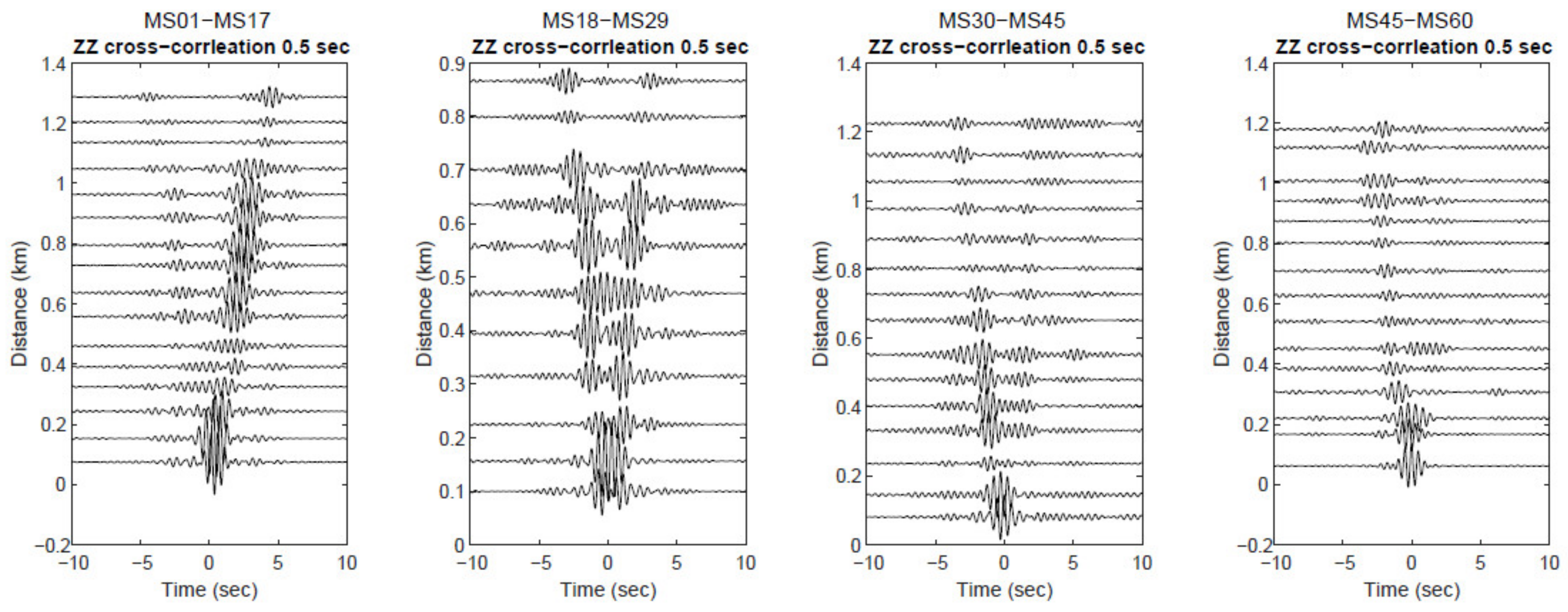
2.1. Ambient Noise Cross Correlations

The data processing procedures of Wang [12] were followed; these use the continuous data stream of the array to obtain the monthly stacked cross-correlation function between stations from the ambient noise signal. First, we divided the vertical component record into segments with lengths of 300 s and converted the data into the frequency domain. Because ambient noise is not flat in the frequency domain, if we do not without the temporal normalization, which reduces the effect of earthquakes, the small resonance is typically not seen. Second, spectral whitening acts to broaden the band of the ambient noise signal in cross-correlations and also combats degradation caused by persistent monochromatic sources [13,14,15]. As aforesaid, to retain the cross-correlation function signal amplitude information on the cross-correlation functions, it is needed to reduce the impact of seismic events. After processing the spectrum whitening, the cross-correlation functions between stations were calculated, and the records were then converted back to the time domain. In the final step, we stacked and normalized the cross-correlation functions into 300 s windows. The array was divided into four sections for displaying the cross-correlation functions. Taking the 0.5 s period as an example, clear Rayleigh waves are observed on both the positive and negative time lags (Figure 2). For enhancing the signal-to-noise (SN) ratio in this study, the positive and negative time lags were stacked, and symmetric cross-correlation functions were constructed and used in this study.

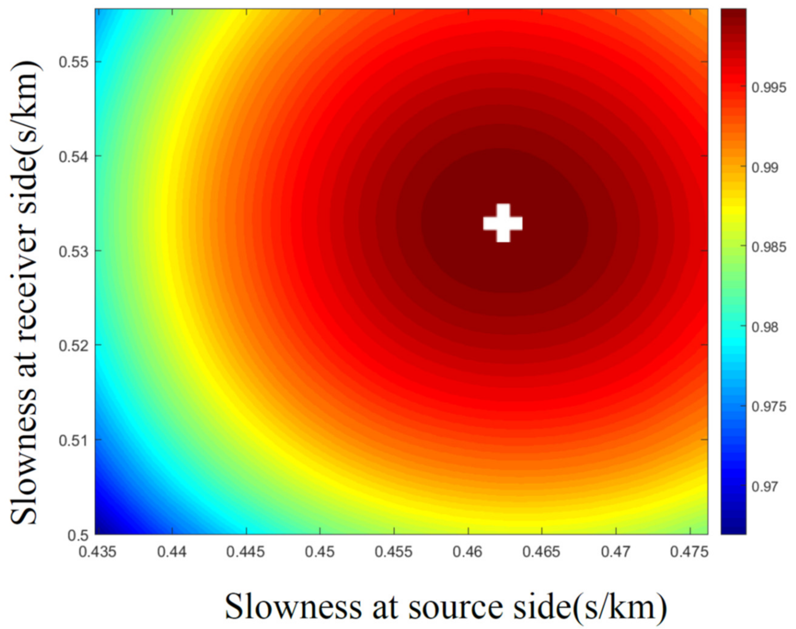
2.2. Double Beamforming Tomography

In the frequency domain, the double beamforming process measures the Rayleigh wave phase velocity between 0.3 s and 0.8 s periods. We adopted 0.35 km as the width of the beam and ensured that there were sufficient numbers of stations under the selected width for obtaining stable results. The array was divided into several beams and one beam was used as the source beam. After the signal was transmitted through the medium, it was received by the other beams, which acted as receiver beams. The interstation distance between every source–receiver pair was required to be longer than one wavelength of the Rayleigh waves in order to satisfy the far-field criterion [16]. The less strict criterion in this study was used to retain a sufficient number of cross-correlation functions for the double beamforming analysis [17,18]. For stacking the fundamental Rayleigh waves, period-dependent velocity thresholds were adopted for cutting and tapering the cross-correlation functions. The period-dependent slowness thresholds were 0.2–5.0 s/km between 0.3 s and 0.8 s (Figure 2). After cutting and tapering, the waveforms were normalized by their maximum amplitudes, transferred to the frequency domain, and stacked and shifted according to the slowness. The beam-stacked cross-correlation functions were then converted back to the time domain and the amplitudes of the envelopes were measured. The grid search technique was used in the source and receiver beams to obtain the best slowness. If the searched slowness closely represents the slowness of the structure at the source side or receiver side, the waveforms will stack constructively, and the stacked waveform will have the largest envelope amplitude. Taking Stations MS22 and MS34 as an example, the maximum amplitude of the envelope of the stacked waveforms with respect to the source beam slowness and receiver slowness was obtained by applying a 2D grid search of the slowness (Figure 3). After repeatedly measuring the slowness with different pairs of source and receiver beams, the mean slowness and its standard deviation were calculated to give final slowness and uncertainty. Figure 4 shows the histograms of repeated measurements of the slowness at Station MS22 for the following three periods: 0.3 s, 0.5 s, and 0.7 s. In the 0.3 s and 0.5 s periods, the statistical results of the slowness show a more centralized distribution resulting in lower uncertainty. For the 0.7 s period, the distribution shows more scatter than for the shorter periods. The mean slowness and the uncertainty at each beam location were used in building the Rayleigh wave phase slowness cross-sections of the entire array for the 0.3 s, 0.5 s, and 0.7 s periods (Figure 5). Significant variations in the gradient at certain locations may be related to variations in the geological structure.

2.3. Shear Velocity Inversion

An iterative least-squares 1D inversion method [19] was applied to obtain the shear wave velocity profile across the Meishan Fault from the Rayleigh wave phase dispersions. At each station along the array, a constant velocity model was used as the initial model and the uncertainties were applied as weights in the inversion process. During the inversion iteration, the Vp/Vs ratio was fixed at 1.80, and the Vp and Vs were updated in each iteration, as well as the density according to the empirical relationship between Vp and density [20]. It was found that the changes in Vs between iterations are not always obvious. After this inversion process was performed at each location to obtain a series 1D Vs model, the 2D Vs profile was finally constructed from all 1D Vs models.

3. Results

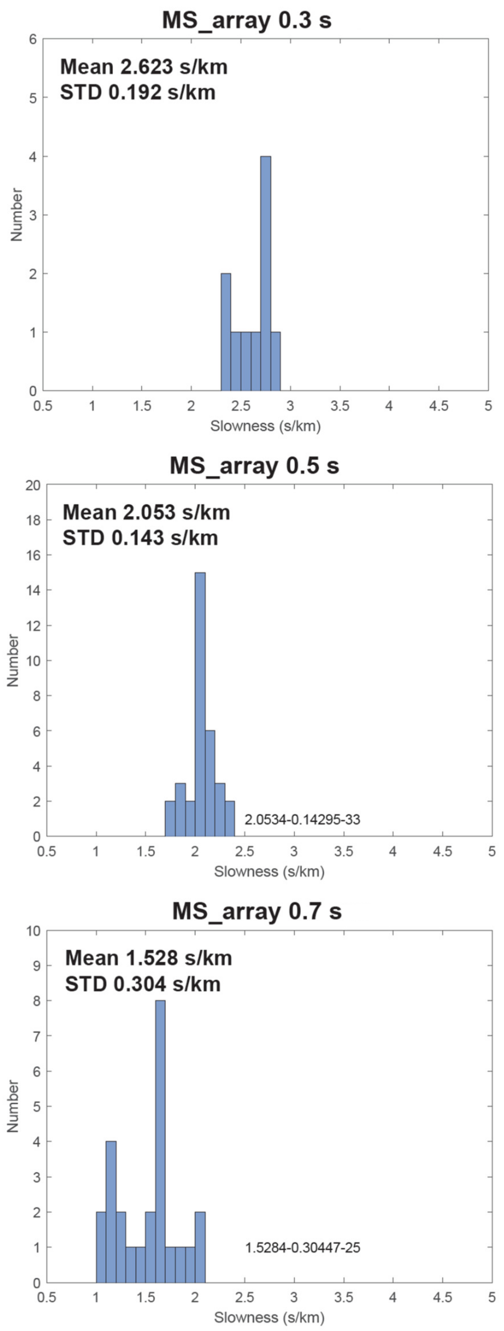
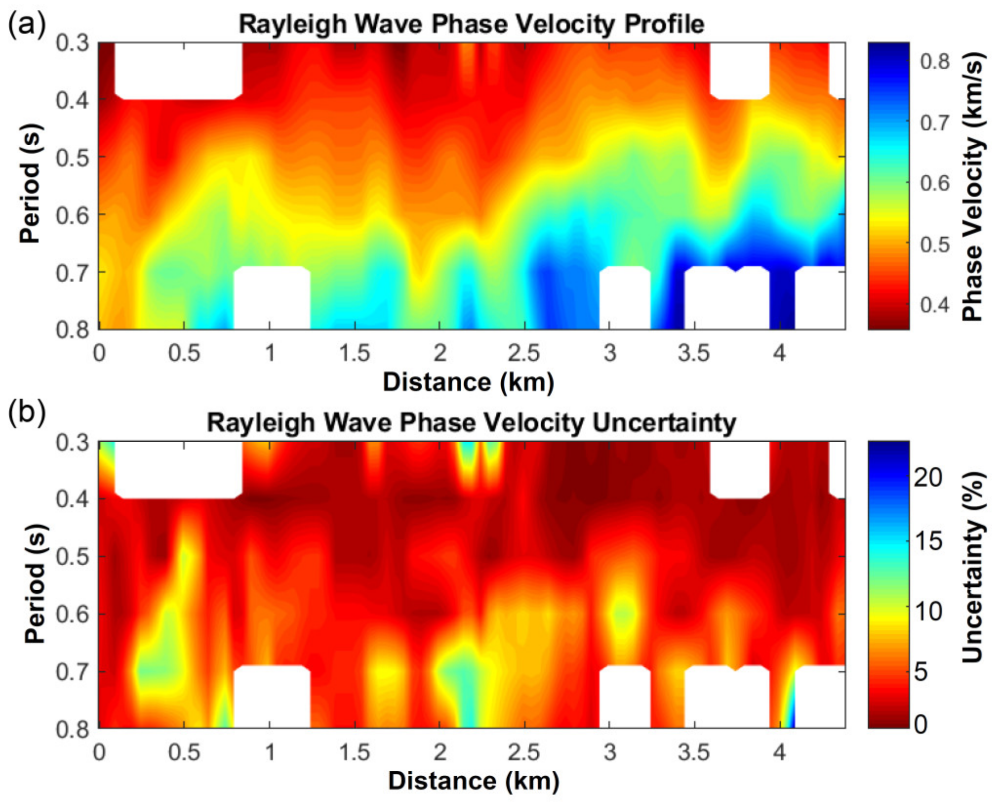
3.1. Phase Velocities and Uncertainties

From the repeated measurements of the slowness and their uncertainty at each location and period (0.3–0.8 s periods), the phase velocity profile of the Rayleigh wave across the Meishan Fault was established (Figure 6). A prominent low-velocity area occurs at 1.1 km to 2.5 km between the 0.3 s and 0.6 s periods. The highest velocities are at the south end of the array and have a greater than 0.6 s period. Overall, the phase velocities increase with the period. There are a few areas with relatively high uncertainties at a distance of approximately 0.4 km between 0.5 s and 0.7 s periods and at approximately 2.2 km for less than 0.4 s periods and greater than 0.7 s periods (Figure 6b). The high uncertainties may be due to the relatively low SN ratios of the observed Rayleigh waves. However, it is not clear that the Rayleigh waves are weak in those areas, and it might be related to the transition between low- and high-velocity materials.

3.2. Phase Velocities and Uncertainties

Figure 7a shows the shear wave velocity profile across the Meishan Fault. In the shear wave velocity profile, velocities generally increase with depth. The Vs is approximately 0.3 km/s at the surface and increases to approximately 1.1 km/s at depth. There are no clear lateral variations at the same depth in the velocity profile; however, the distribution of Vs shows a similar pattern to the phase velocity profile (Figure 6a) of the Rayleigh wave. For example, the contour of Vs = 0.6 km/s from 1.1 to 2.5 km along the profile and between 0.1 km and 0.15 km in-depth, and the U-shaped features mimic the Rayleigh wave phase velocities. Figure 7b shows the perturbations of the Vs profile and the perturbations relative to the average shear velocity at each depth. In the perturbations of the Vs profile, a clear transition between low-velocity and high-velocity materials is observed at approximately 2.5 km distance along the profile.

4. Discussion

The Chiayi blind fault divides the Meishen Fault area into the following two parts: a coastal plain to the west and an uplifted platform to the east [21,22]. The coastal plain mostly consists of soft alluvial strata, and the uplifted platform is covered by Late Pleistocene to Holocene laterite and alluvium deposits [21]. While the Meishan Fault is generally recognized as a right-lateral strike-slip fault, based on the simulated results of historical seismic data, Liao [23] believes that the focal mechanism of the 1906 Meishan earthquake was that of an oblique thrust fault mechanism with a strike oriented in the NE-SW direction and with a small right-lateral component. In addition, the transient location of the Meishan Fault trace is also controversial. One location is indicated by the CGS and passes through the northwest side of CCU, and the other location, indicated by Omori [3], passes through the southeast side of the campus.

The distribution of the array in this study is shown in Figure 1. The seismic array passes through the Meishan Fault and has a length of approximately 4.8 km. The north part of the array is parallel to the distribution of eight geological drilled wells and the profile of seismic surveys obtained by Chen [21], and the south part of the array intersects the seismic survey profile obtained by Wang and Li [24]. On the basis of the drilling results, Chen [21] confirmed that the Meishan Fault is a right-lateral strike-slip fault. They also showed that there is substantial deformation of the strata in the wells near the trace of the Meishan Fault, indicating that the Meishan Fault might pass between these wells. Furthermore, the shear wave velocity profile above 20 m, as obtained from seismic surveys, shows significant lateral variation in velocity, and this is consistent with the location of a large amount of deformation between the strata. The velocity profile of Chen [21] indicates that Vs gradually increases from approximately 0.1 km/s at the surface to approximately 0.37 km/s at 20 m in depth. The Vs in this study are approximately 0.3–0.4 km/s above 50 m depth. Therefore, the absolute value of Vs is consistent with the results of the previous studies in the shallow part of the profile. Moreover, the lateral velocity variation in Chen [21] occurs at 1.1 km along the profile of this study, which also shows significant variations in the shallow part of the perturbation profile at this point (Figure 7b). In conclusion, we believe that the Meishan Fault passes through the northwest side of CCU.

Systematic research on the distribution, geometry, and kinematics of the flower structures, including the fault systems formed at different times and controlled by different factors, suggests that the faults in the stepover zone are very different from a major strike-slip fault. In general, the stress orientation is not parallel to the strike of the strike-slip fault [25,26]. Thus, the fault might feature bends and form stepovers [1], and the formation of the flower structures in the stepover zone is easier [25,26]. The Meishan Fault is a right-lateral strike-slip fault, and its fault trace is a right-ascending step. Therefore, it is likely that this is a compressed flower structure along the Meishan Fault; this phenomenon has been observed in several studies [8,24].

Wang and Li [24] finished four profiles, Profiles A, B, C, and D, derived from a reflection seismic survey. The locations from the northeast to southwest of these profiles are Meishan (Profile A), Zhongkeng (Profile B), Nanhua University (Profile C), and CCU (Profile D). Profile A shows that the stratum is bent in a reverse U-shape, and this phenomenon is known as the Xiaomei anticline. Profile A also shows the compressional flower structure in the area where the Meishan Fault was active. A similar seismic survey result was obtained by Shih [8] at the same location. In the Zhongkeng region (Profile B), the uplift caused by the flower structure can also be seen. Further southwest at Nanhua University, Profile C, which is along the Sandie River, shows similar structures to other profiles, including the flower structure, whose location is consistent with the fault trace obtained by Omori [3]. Profile D passes through the southwest side of CCU, and its results demonstrate that there is barely a horizontal stratum in the north part of Profile D. The stratum has a slight uplift in the south part of Profile D, and this is interpreted as the transient position of the Maishan fault in previous studies [3,24]. However, there is no obvious flower structure in Profile D. Profile D intersects the seismic array in this study at approximately 2.3–2.5 km, and this intersection is also near the stratum where there is a slight uplift. At this intersection with the perturbation profile, a clear and nearly vertical velocity transition could be observed. Wang and Li [24] interpreted this boundary as the location of the Meishan Fault obtained by Omori [3]; however, this boundary is also near the branch fault (Chentsoliao fault). In our results, the velocity transition is closer to the location of the Chentsoliao Fault. Thus, we believe that the slight uplift of the stratum and the velocity transition may have been caused by the Chentsoliao Fault instead of the Meishan Fault as suggested by Omori [3].

The width of the fault damage zone is related to the cumulative displacement of the fault. The large variation in fault width may be caused by the roughness properties of the fault [27,28]. Otherwise, the faults, which feature bends or stepovers, increase stresses, resulting in a wider damage zone [1]. The resulting Vs in the damage zone is at approximately 0.3–0.6 km/s [29]. In accordance with these previous studies, the Vs profile in the present study implies that the Meishan Fault may be broad, and possibly over 3 km in width. This phenomenon has been noted in previous seismic surveys [30,31,32]. These investigators found that numerous flower structures are widespread beneath the Xiaomei anticline. However, our study area is covered by thick laterite and alluvium deposits, and the Vs in deposits (VS = ~0.3–0.4 km/s) is similar to the Vs in the damage zone. Thus, it is difficult to distinguish the damage zone width based on the Vs distribution of this profile. Zheng [33] also presented 3D Vs tomography of the Meishan Fault zone. Since its resolution is limited by the interstation distance (approximately 2 km), the tomography cannot reveal the effects of the numerous flower structures beneath the Xiaomei anticline. However, their results demonstrate clear velocity variations between the two sides of the Meishan Fault, and this is consistent with the perturbation profile in the present study.

5. Conclusions

This study used short period (0.3–0.8 s) double beamforming tomography from ambient noise data to obtain the shallow velocity structures (<300 m) across the Meishan Fault. In the shear wave velocity profile, the velocities generally increase with depth, from 0.3 km/s at the surface to 1.1 km/s at depth. Although we could not distinguish the fault zone width due to the thick laterite covering the study area, the results provide local-scale seismic imaging that agrees with the geological and regional-scale tomography results. According to the results of this study, we believe that the Meishan Fault has propagated through the northwest side of the CCU as indicated by the CGS, and the velocity transition of the perturbation profile may be caused by a branch fault, the Chentsoliao Fault. This study demonstrates that the ambient noise double beamforming method is an effective tool for imaging the detailed shallow structure along a dense seismic array.

References

1. Finzi, Y.; Hearn, E.H.; Ben-Zion, Y.; Lyakhovsky, V. Structural properties and deformation patterns of evolving strike-slip faults: Numerical simulations incorporating damage rheology. Pure Appl. Geophys. 2009, 166, 1537–1573. [Google Scholar] [CrossRef] [Green Version]
2. Meyer, S.E.; Kaus, B.J.P.; Passchier, C. Development of branching brittle and ductile shear zones: A numerical study. Geochem. Geophys. Geosyst. 2017, 18, 2054–2075. [Google Scholar] [CrossRef]
3. Omori, F. Preliminary note on the Formosa earthquake of March 17, 1906. Bull. Imp. Earthq. Inves. Comm. 1907, 2, 53–71. [Google Scholar]
4. Bonilla, M.G. A review of recently active faults in Taiwan. In U.S. Geological Survey Open-File Report 75-41, Version 1.1; USGS: Reston, VA, USA, 1975; p. 43. [Google Scholar]
5. Hsu, T.L.; Chang, H.C. Quaternary faulting in Taiwan. Mem. Geol. Soc. China 1979, 3, 155–165. [Google Scholar]
6. Lin, C.-W.; Chang, H.-C.; Lu, S.-T.; Shih, T.-S.; Huang, W.-C. An Introduction to the Active Faults of Taiwan, 2nd ed.; Central Geological Survey Special Publication: New Taipei, Taiwan, 2000; pp. 1–122. (In Chinese)
7. Chen, H.-W.; Shih, T.-S.; Shao, P.-H.; Huang, P.-H.; Chang, H.-C. The Study of Meishan Fault from Dalin and Zhongkeng Quaterary Strata Profiles; Annual Report of Central Geological Survey; Central Geological Survey: New Taipei, Taiwan, 2001; pp. 12–15. (In Chinese)
8. Shih, R.-C.; Chen, P.-H.; Lu, M.-T.; Chen, W.-S. Construction of Active Fault Database Plan Form Seismic and Geological Surveys—Shallow Geophysical Exploration (1/5); Annual Report of Central Geological Survey; Central Geological Survey: New Taipei, Taiwan, 2002; pp. 1–166. (In Chinese)
9. Huang, C.-Y.; Shyu, C.-T.; Lin, S.B.; Lee, T.-Q.; Sheu, D.D. Marine geology in the arc-continent collision zone off southeastern Taiwan: Implications for Late Neogene evolution of the Coastal Range. Mar. Geol. 1992, 107, 183–212. [Google Scholar] [CrossRef]
10. Chen, W.-S.; Yang, C.-C.; Shih, R.-C.; Yang, H.-C.; Yan, Y.-C.; Chen, Y.-G.; Chang, H.-C.; Lin, W.-H.; Lee, Y.-H.; Shih, T.-S.; et al. Structural Characteristics of the Chiuchiungkeng Fault. Cent. Geol. Surv. Spec. Publ. 2003, 14, 123–139. (In Chinese) [Google Scholar]
11. Chen, W.-S.; Yu, N.-T.; Yang, H.-C. The Characteristics Investigation of Important Active Faults Research Project-Analysis and Evaluation of Active Faults (3/4); Final Report of Central Geological Survey; Central Geological Survey: New Taipei, Taiwan, 2013; pp. 1–98. (In Chinese)
12. Wang, Y.; Lin, F.C.; Ward, K.M. Ambient noise tomography across the Cascadia subduction zone using dense linear seismic arrays and double beamforming. Geophys. J. Int. 2019, 217, 1668–1680. [Google Scholar] [CrossRef]
13. Bensen, G.D.; Ritzwoller, M.H.; Barmin, M.P.; Levshin, A.L.; Lin, F.; Moschetti, M.P.; Shapiro, N.M.; Yang, Y. Processing seismic ambient noise data to obtain reliable broad-band surface wave dispersion measurements. Geophys. J. Int. 2007, 169, 1239–1260. [Google Scholar] [CrossRef] [Green Version]
14. Harmon, N.; Gerstoft, P.; Rychert, C.A.; Abers, G.A.; Salas de La Cruz, M.; Fischer, K.M. Phase velocities from seismic noise using beamforming and cross correlation in Costa Rica and Nicaragua. Geophys. Res. Lett. 2008, 35, L19303. [Google Scholar] [CrossRef] [Green Version]
15. Gatto, M.P.A.; Montrasio, L.; Zavatto, L. Experimental Analysis and Theoretical Modelling of Polyurethane Effects on 1D Wave Propagation through Sand-Polyurethane Specimens. J. Earthq. Eng. 2021, 1–24. [Google Scholar] [CrossRef]
16. Wang, Y.; Lin, F.-C.; Schmandt, B.; Farrell, J. Ambient noise tomography across Mount St. Helens using a dense seismic array. J. Geophys. Res. Solid Earth 2017, 122, 4492–4508. [Google Scholar] [CrossRef]
17. Yao, H.; van Der Hilst, R.D.; De Hoop, M.V. Surface-wave array tomography in SE Tibet from ambient seismic noise and two-station analysis—I. Phase velocity maps. Geophys. J. Int. 2006, 166, 732–744. [Google Scholar] [CrossRef] [Green Version]
18. Yao, H.; Beghein, C.; Van Der Hilst, R.D. Surface wave array tomography in SE Tibet from ambient seismic noise and two-station analysis-II. Crustal and upper-mantle structure. Geophys. J. Int. 2008, 173, 205–219. [Google Scholar] [CrossRef] [Green Version]
19. Herrmann, R.B. Computer programs in seismology: An evolving tool for instruction and research. Seismol. Res. Lett. 2013, 84, 1081–1088. [Google Scholar] [CrossRef]
20. Yun, K.Y. A Study in the Conversion between P-Wave Velocity and Density Models of Yunlin and Chiayi Areas, Taiwan. Master’s Thesis, National Chung Cheng University, Chiayi, Taiwan, 2018. (In Chinese). [Google Scholar]
21. Chen, W.-S.; Yang, C.-C.; Yang, H.-C.; Wu, L.-C.; Lin, C.-W.; Chang, H.-C.; Shih, R.-C.; Lin, W.-H.; Lee, Y.-H.; Shih, T.-S.; et al. Tectono-geomorphologic studies in the Chiayi-Tainan region in southwestern Taiwan and its implications for active structure. Bull. Cent. Geol. Surv. 2004, 17, 53–78. (In Chinese) [Google Scholar]
22. Chen, W.-S.; Yeh, M.-G.; Yang, C.-C.; Shih, R.-C.; Lin, C.-W.; Hou, C.-S. Structural Studies of the Meishan Fault, Southwest Taiwan. Bull. Cent. Geol. Surv. 2006, 19, 135–151. (In Chinese) [Google Scholar]
23. Liao, Y.W.; Ma, K.F.; Hsieh, M.C.; Cheng, S.N.; Kuo-Chen, H.; Chang, C.P. Resolving the 1906 Mw 7.1 Meishan, Taiwan, Earthquake from Historical Seismic Records. Seismol. Res. Lett. 2018, 89, 1385–1396. [Google Scholar] [CrossRef] [Green Version]
24. Wang, C.-Y.; Lee, Y.-H. The Investigation form Seismic Survey; National Central University: Taoyuan, Taiwan, 2005. (In Chinese) [Google Scholar]
25. Wilcox, R.E.; Harding, T.P.; Seely, D.R. Basic wrench tectonics. Aapg Bull. 1973, 57, 74–96. [Google Scholar]
26. Woodcock, N.H.; Fischer, M. Strike-slip duplexes. J. Struct. Geol. 1986, 8, 725–735. [Google Scholar] [CrossRef] [Green Version]
27. Dieterich, J.H.; Smith, D.E. Nonplanar faults: Mechanics of slip and off-fault damage. Pure Appl. Geophys. 2009, 166, 1799–1815. [Google Scholar] [CrossRef]
28. Fang, Z.; Dunham, E.M. Additional shear resistance from fault roughness and stress levels on geometrically complex faults. J. Geophys. Res. Solid Earth 2013, 118, 3642–3654. [Google Scholar] [CrossRef]
29. Wang, Y.; Allam, A.; Lin, F.C. Imaging the fault damage zone of the San Jacinto Fault near Anza with ambient noise tomography using a dense nodal Array. Geophys. Res. Lett. 2019, 46, 12938–12948. [Google Scholar] [CrossRef]
30. Sun, W.-H. The Three-Dimensional Seismic Interpretation of Structure of the Meishan Fault Zone. Master’s Thesis, National Chung Cheng University, Chiayi, Taiwan, 2015. (In Chinese). [Google Scholar]
31. Tsao, H.-C. Subsurface Image of the Meishan Fault and in Nearby Structure by Using the Seismic Reflection Data. Master’s Thesis, National Chung Cheng University, Chiayi, Taiwan, 2017. (In Chinese). [Google Scholar]
32. Huang, W.-H. Integrated Interpretation of the Structure of the Meishan Fault by Using Seismic Exploration Data. Master’s Thesis, National Chung Cheng University, Chiayi, Taiwan, 2018. (In Chinese). [Google Scholar]
33. Zheng, J.-Y. 3-D Shear Wave Shallow Crustal Structure at Meishan Fault Zone Using Ambient Noise Tomography. Master’s Thesis, National Central University, Taoyuan, Taiwan, 2018. (In Chinese). [Google Scholar]
Figure 1. A topographic map showing the locations of the Meishan Fault, seismic stations, and the National Chung Cheng University (CCU) region. The blue box represents the CCU region, and the red and black lines indicated the fault traces of the Meishan Fault obtained by the CGS and Omori [3], respectively. The array of the sixty smartsolo geophones is represented by white triangles. The inset map shows the study area (Taiwan).
Applsci 12 05847 g001
Figure 2. Vertical to vertical component cross correlation from the source station to the receiver stations for each section. The first section is north of the Meishan Fault (MS01−MS17), and the next section (MS18−MS29) is inside CCU. The third (MS30−MS45) and fourth (MS45−MS60) sections are south of CCU.
Applsci 12 05847 g002
Figure 3. The maximum amplitude of the envelope of the stacked waveforms with respect to source beam slowness and receiver slowness for Stations MS22 and MS34, taken as an example. The color bar represents the amplitude of the stacked waveforms for each slowness, and the white cross indicates the location of the maximum amplitude.
Applsci 12 05847 g003
Figure 4. Histograms of repeated measurements of the slowness at Station MS22 at periods of 0.3 s, 0.5 s, and 0.7 s.
Applsci 12 05847 g004
Figure 5. The slowness measurements along the entire array at periods of 0.3 s, 0.5 s, and 0.7 s. The error bars show the uncertainties of the mean slowness.
Applsci 12 05847 g005
Figure 6. (a) The Rayleigh wave phase velocity profile and (b) its uncertainty profile as measured by the double beamforming method.
Applsci 12 05847 g006
Figure 7. (a) Cross-section of the shear velocities across the Meishan Fault. (b) Perturbations of the Vs profile, and perturbations relative to the average shear velocity at each depth.
Applsci 12 05847 g007
Publisher’s Note: MDPI stays neutral with regard to jurisdictional claims in published maps and institutional affiliations.