On the Communication Performance of Airborne Distributed Coherent Radar

Abstract

Compared with a monostatic radar, airborne distributed coherent radar (ADCR) has been widely applied thanks to its flexibility, greater degree of freedom, stronger detection, and anti-jamming ability. Unlike distributed ground-based radar, the precondition for ADCR to perform tasks is maintenance of stable wireless communication links among the unmanned aerial vehicles (UAVs). Therefore, the communication channel modeling of ADCR is very important. This paper mainly analyzes the performance of a communication system composed of radar UAVs, communication UAV (relay), and ground base station. The probability density function (PDF) and outage probability (OP) of signal-to-noise ratio (SNR) at the ground terminal are derived analytically in the cases of transmission power error, UAV position error, and multi-path fading. Numerical simulation shows the validity of the derived results.

1. Introduction

The detection ability and anti-jamming ability of conventional monostatic radars are relatively weak. The complex electromagnetic environment of modern society necessitates greater requirements for the detection ability of radar [1]. Under the existing technical conditions, detection capability can be improved by increasing antenna aperture and signal bandwidth, but this will create problems such as large radar volume, limited mobility, high manufacturing cost, and difficult later maintenance [2]. ADCR can overcome the above shortcomings and significantly improve radar detection ability and anti-jamming ability [3,4]. It is usually composed of multiple radars with different functions and information fusion centers [5]. Compared with ground-based radar, ADCR generally offers the following advantages:

• Radars with different frequency bands, power, polarization, and antenna patterns can be combined systematically to detect targets from multiple angles and in various ways. Meanwhile, coherent detection can also be realized. These advantages can improve the detection probability of the target [6].
• When a small number of radars are subject to inevitable electronic attack or failure, other radars can quickly form an effective detection network, which greatly improves the anti-jamming ability of the radar network [7].
• Compared with ground-based radar, ADCR is usually smaller, more flexible, and easier to deploy [8].

However, unlike distributed ground-based radar, the prerequisite for an ADCR radar to perform its mission is to maintain a stable communication connection [9]. This is necessary for the network to perform tasks independently or to be controlled by the ground station in real time. Meanwhile, compared with distributed ground-based radar, the ADCR communication system must be connected wirelessly, which is more unreliable than wired communication. The factors that obviously affect the performance of airborne radar communication system mainly include the following three aspects:

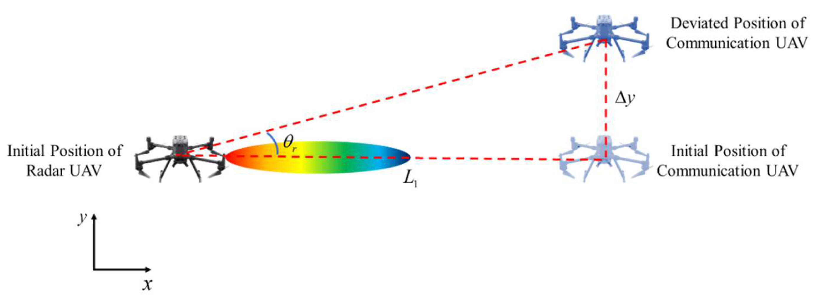
• UAV position fluctuation: Ground-based radar is usually fixed, while ADCR is usually affected by forces such as wind, with its position fluctuating [10]. Taking the communication between UAVs as an example, communication usually depends on the directional antenna, and the mainlobe of the transmitting antenna should point to the connecting direction between the transmitter and the receiver by default. However, the fluctuation of the transmitter or the receiver will cause the receiver to deviate from the mainlobe of the transmitter, which will further cause the antenna gain of the communication link to decline and affect the communication performance.
• Limited load of UAV: Unlike high-power ground-based radar, the load of ADCR is usually very limited [11,12]. This mainly includes the energy carried by UAVs and their limited size. Limited energy leads to limited transmitting power and motion capability of UAVs, which will lead to limited communication coverage and motion range. Limited size often leads to performance limitations related to size and area. For example, fewer antenna elements will lead to wider mainlobe width. The limited size may also affect the performance of some precision components, such as the stability of the transmitter’s power amplifier [12,13,14].
• Nature of wireless channel propagation: Since ADCR cannot rely on wired communication in the same way as ground-based radar, shadow fading, multi-path fading, and propagation loss will affect communication performance [15].

In view of the significant difference between ADCR and ground-based radar in the analysis of communication performance, it is important to build a comprehensive and accurate channel model for ADCR. At present, the performance analysis work of UAV communication system is emerging in endlessly. We divide these works into two main categories: one is to focus on the impact of antennas and beams on communication performance; the second is to focus on the impact of cascading and fading on communication performance.

Antenna and beam: the impact of beam misalignment caused by fluctuating UAV position on communication performance is studied. Zhangyu Guan et al. studied the challenges faced by UAVs when applying millimeter wave or terahertz directional transmission [16]. They pointed out that the misalignment between the transmitting and receiving antennae of the UAVs could easily lead to communication outage in many outdoor measurement experiments. Weizhi Zhong et al. [17] focused on formation of an adaptive beam to overcome the unstable beam pointing between UAVs. They combined the feedback information of beam deviation measured by different sensors, the expected data rate and greedy geometry algorithm to propose a beam design method. Fouda Abdurrahman et al. [18] analyzed the impact of beam misalignment on communication performance in non-orthogonal multiple-access downlink systems. In addition, Mohammad Taghi Dabiri et al. also conducted a lot of in-depth research on the position fluctuation of UAV. For example, in [19] they established the position fluctuation of UAV as Gaussian random variable, and modeled the channel fading with Nakagami distribution. The analytic expression of OP was derived under three different topology models. Mohammad Taghi Dabiri et al. further enriched and improved previous work in [20], and expanded the antenna model from the original uniform linear array to any planar array. On the basis of performance analysis, they also studied the optimal antenna pattern and the optimal geometric position of the relay UAV.

Cascading and fading: This part mainly focuses on the cascading between different communication links, and considers the impact of different shadow fading or multi-path fading on communication performance. At present, the dual-hop link is the most studied field. For example, Yang Liang et al. conducted a lot of research on the dual-hop system in an urban environment. In [21], they proposed a communication system in which an UAV acted as a relay. Yang Liang also conducted a lot of in-depth research on the performance of the dual-hop communication system combining UAV and intelligent reflecting surface (IRS). For example, in [22], the IRS fixed on the building was used to improve the severe fading between the ground transmitting source and UAV. The OP, bit error rate and ergodic channel capacity at the destination terminal were derived. In addition, Xiaomin Chen et al. [23] studied the performance of multi-hop communication links where UAVs acted as relays. Considering the propagation loss, shadowing, and multi-path fading of the communication system, the OP and other performances of the communication system composed of ground-to-air (G2A), air-to-air (A2A), and air-to-ground (A2G) were derived. The rationality of the proposed OP was verified by numerical simulation under different terrain conditions (such as hills, mountains, and oceans).

From the above research, the following two deficiencies can be summarized:

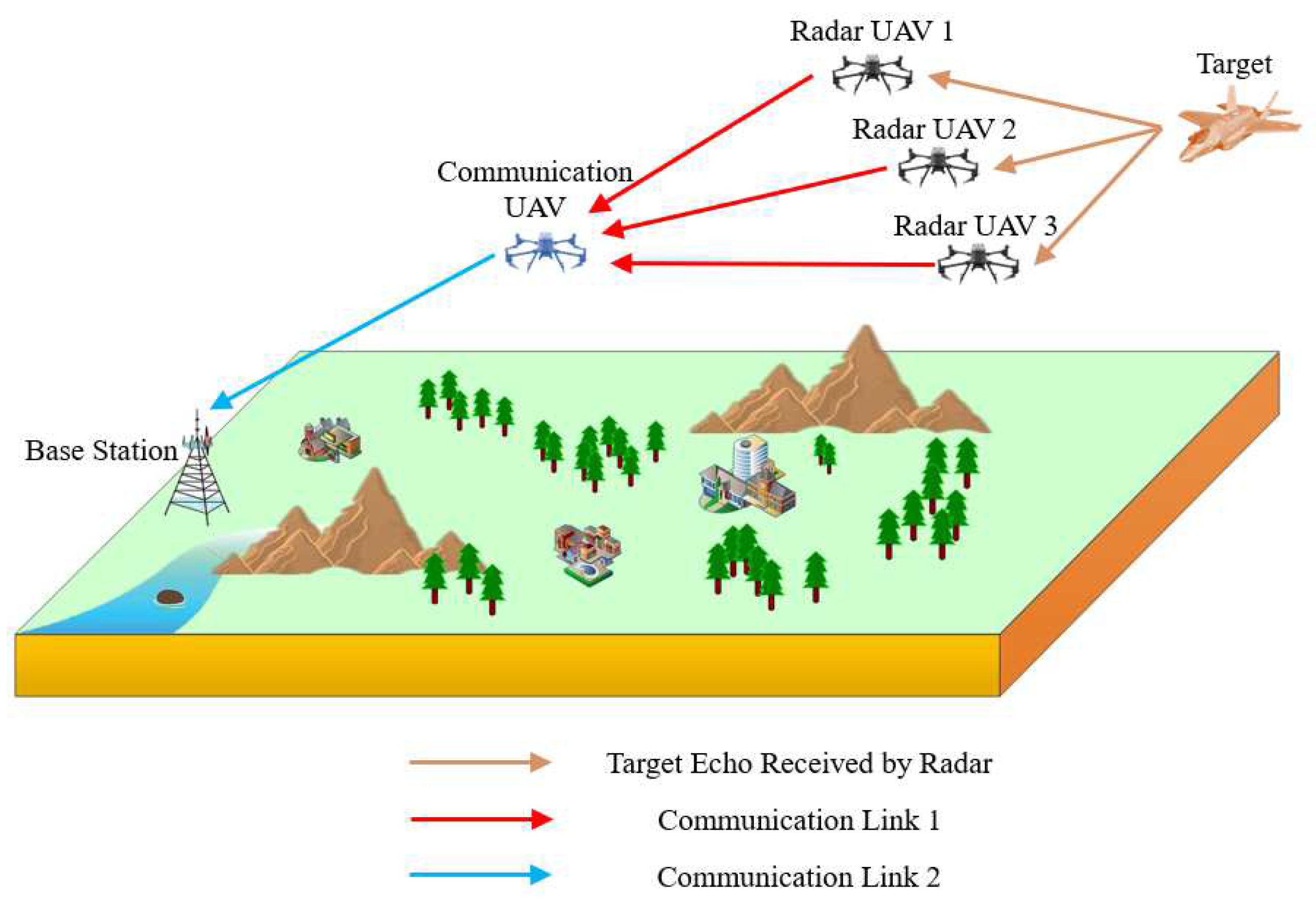
• At present, there is still little research into communication performance analysis for ADCR. Since the target detection by ADCR is usually coherent, and the data acquired by radar UAVs needs to be sent (possibly through relay) to the ground information fusion center for processing. In this case, if the clocks between UAVs can keep strict synchronization, the communication signals transmitted by each radar UAV can be directly summed at the communication UAV. Therefore, the topology of ADCR is usually complex. Thus, the above existing research and conclusions are not directly applied. This will be explained carefully in the modeling of Section 2.
• At present, few studies comprehensively consider factors such as UAV transmitting power error [24], UAV position error [19,20,25], multipath fading [26,27]. Most research only considers one or several of them.

Based on the above research status and analysis, this paper aims to build a channel model which is suitable for ADCR communication system and covers a wide range of factors. Meanwhile, this paper is also devoted to deriving the closed-form expression of OP under this channel model. Numerical results will verify the rationality of the theoretical expressions.

The main contributions of this paper are as follows:

• A channel model suitable for ADCR communication systems under coherent conditions is constructed. Compared with the existing research on communication performance analysis, our proposed model features two innovations: First, the load of radar UAV and communication UAV is limited, which leads to the performance error of their power amplifiers. We use the model based on noncentral chi-squared distribution to express their transmission power error, and cascade it with other random variables in the scenario, such as multi-path fading, antenna pointing error, etc., which makes up for the shortcomings of the existing work. Second, considering the coherent detection of target by radar UAV, the communication signal can also be directly accumulated at the communication UAV. This performance analysis mode of radar-communication cooperative optimization is rarely seen in the existing research.
• By approximating the Rician distribution and the noncentral chi-squared distribution, the analytic expression of OP at the ground base station is derived. Noncentral chi-squared distribution and Rician distribution are usually expressed in the form of modified Bessel function, which is not conducive to cascading with random variables such as multi-path fading. Therefore, we use an approximate expression to represent noncentral chi-squared distribution and Rician distribution respectively.
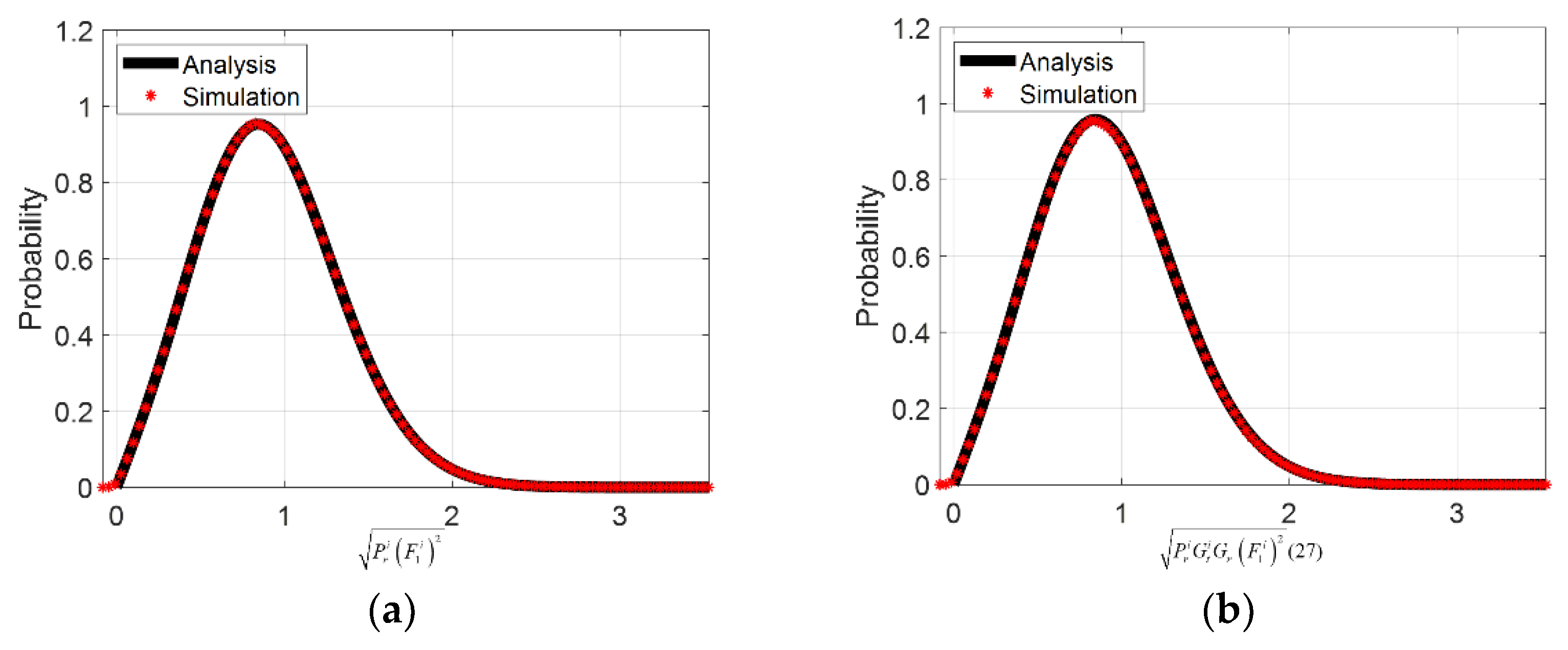
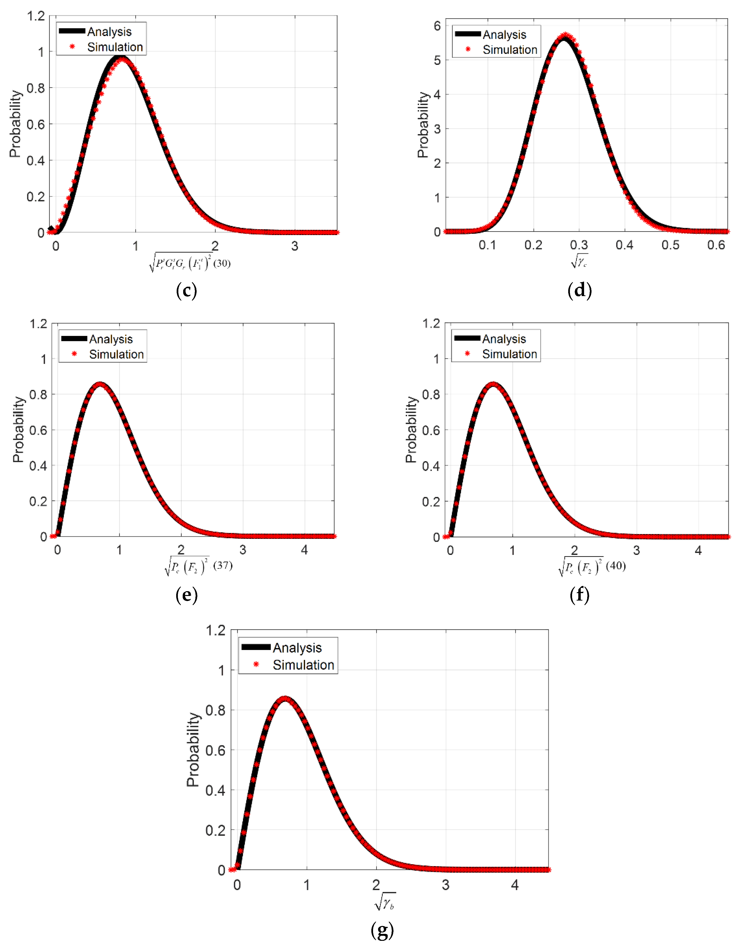
• The rationality of the proposed closed-form expression is verified by numerical simulation.

The rest of this paper is organized as follows: in Section 2, the communication system model based on ADCR is established, including the topology of the communication system, statistical model of errors and fading. On this basis, Section 2 derives the analytical expressions of the OP at the ground base station. The corresponding numerical simulation results are presented in Section 3, which proves the correctness of the theoretical derivation. Section 4 summarizes the full paper and analyzes the work in the future.

2. Materials and Methods

In this section, we mainly present the system structure of ADCR communication system, analyze the basic statistical model of some random variables such as the amplitude of multi-path fading, and derive the OP of the whole system by mathematical methods.

2.1. System Model

In this subsection, we build the overall topology of the ADCR communication system. On this basis, we also give the statistical models of UAV transmitting power (with errors), UAV position (with errors), and multi-path fading, which can be used for the subsequent derivation of the analytical expression of OP in Section 2.2.

2.1.1. The Overall Topology of the ADCR Communication System

Figure 1 shows the topology of the ADCR communication system. As shown in the figure, the communication system consists of several radar UAVs, a communication UAV, and a ground base station. Each radar UAV sends electromagnetic waves to detect the target and receives a target echo. The target echo is represented by a brown arrow in Figure 1. At this time, each radar UAV needs to transmit the echo information to the ground base station. However, since the terrain on the ground is too complex and the radar UAV is far from the ground base station, at least one communication UAV is required to act as a relay. To simplify the analysis, we only set up one communication UAV. In general, the signal received by the communication UAV from each radar UAV may be the echo signal, or it may be the result of the preliminary signal processing by the radar UAV (such as the target range, velocity, etc.). In this paper, the radar UAV transmits the coherent target echo signal to the communication UAV. The communication UAV adopts the decode-and-forward (DF) mode for the information transmitted by each radar UAV, and forwards the information to the ground base station. The communication link between the radar UAV and the communication UAV is named communication link 1, and the communication link between the communication UAV and the ground base station is named communication link 2.

It should be emphasized that we assume that each radar UAV performs a coherent detection task for the target, and each radar UAV is of the ability to perform coherent processing on the echo signal. At this time, the echoes obtained by each radar can be directly summed at the communication UAV. That is to achieve coherent accumulation of echoes and provide a great gain for the final target detection at the base station. Since each radar UAV transmits coherent radar echoes to the communication UAV, if the clocks of all UAVs are synchronized, these communication signals can also be directly summed at the communication UAV.

For the convenience of subsequent representation, we define the following variables: the number of radar UAVs is $N_{radar}$, the corresponding transmitting power of $i$-th radar UAV is $P_r^i$ (where $i=1,2,\cdots ,N_{radar}$), and the power gain of transmitting antenna is $G_t^i$. The transmitting power of the communication UAV is $P_c^{}$, and the power gain of the receiving antenna is $G_r^{}$. For the communication link between the $i$-th radar UAV and the communication UAV, its corresponding fading is $F_1^i$ and the distance is $L_1^i$. For the communication link between the communication UAV and the base station, its corresponding fading is $F_2^{}$ and the distance is $L_2^{}$. The noise variance introduced by the receiver of the communication UAV is $N_c$, and the noise variance introduced by the receiver of the base station is $N_b$. In order to simplify the problem, we assume that the propagation coefficients of all paths are $\alpha$. We assume that for each radar UAVs, $G_r^{}$ is an independent random variable. Meanwhile, since the radar UAV is usually far away from the communication UAV, we believe that there is $L_1\approx L_1^i$, that is, the distance between each radar UAV and the communication UAV is roughly the same. Since the receiving antenna of the base station is usually large in size and the effective receiving range of angle arrival is often wide, the impact of the position error of the communication UAV on the communication performance can be ignored.

Based on the above definition, it is necessary to determine the receiving signal model at the communication UAV and base station under the DF mechanism. At this time, the receiving signal model of the communication UAV is:

$$y_c=\left({\displaystyle \sum _{i=1}^{N_{radar}}\sqrt{\frac{P_r^i{G}_t^i{G}_r^{}{\left(F_1^i\right)}^2}{{\left(L_1\right)}^{\alpha }}}}\right)x_r+n_c,$$

(1)

where $x_r$ is the communication signal carrying the coherent radar echo information, and $n_c$ is the noise. The receiving signal model of the base station is:

$$y_b=\sqrt{\frac{P_c^{}{\left(F_2^{}\right)}^2}{{\left(L_2\right)}^{\alpha }}}{x}_c+n_b,$$

(2)

where $x_c$ is the transmitting signal of the communication UAV and $n_b$ is the noise. According to (1) and (2), the instantaneous SNR ${\gamma }_c$ at the communication UAV and the instantaneous SNR ${\gamma }_b$ at the base station can be obtained by

$${\gamma }_c={\left({\displaystyle \sum _{i=1}^{N_{radar}}\sqrt{P_r^i{G}_t^i{G}_r^{}{\left(F_1^i\right)}^2}}\right)}^2\frac{1}{N_c{\left(L_1\right)}^{\alpha }}$$

(3)

$${\gamma }_b=\frac{P_c^{}{\left(F_2^{}\right)}^2}{N_b{\left(L_2\right)}^{\alpha }}$$

(4)

2.1.2. Statistical Model of $P_r^i$ and $P_c$

Due to the limitation of UAV load, the power amplifier output of each UAV may be unstable. Therefore, in this subsection, we will give the transmitting power model of radar UAV and communication UAV. Since power is closely related to amplitude, we define the amplitude factor corresponding to the $i$-th radar UAV as $A_r^i$, and the amplitude factor corresponding to the communication UAV as $A_c^{}$. So obviously there is $P_r^i={\left(A_r^i\right)}^2$, $P_c^{}={\left(A_c^{}\right)}^2$. If $A_r^i$ follows the Gaussian distribution with mean ${\mu }_r^i$ and variance ${\left({\sigma }_r^i\right)}^2$. $A_c^{}$ follows the Gaussian distribution with mean ${\mu }_c$ and variance ${\sigma }_c^2$. i.e., $A_r^{}~\mathcal{N}\left({\mu }_r^i,{\left({\sigma }_r^i\right)}^2\right)$ and $A_c^{}~\mathcal{N}\left({\mu }_c,{\sigma }_c^2\right)$. We define $B_r^i=A_r^i/{\sigma }_r^i$ and $B_c^{}=A_c^{}/{\sigma }_c^{}$. Then ${\left(B_r^i\right)}^2$ follows the noncentral chi-squared distribution with scale parameter ${\lambda }_r^i={\left(\frac{{\mu }_r^i}{{\sigma }_r^i}\right)}^2$ and degree of freedom 1. The PDF of ${\left(B_r^i\right)}^2$ is:

$${\mathit{f}}_{{\left(B_r^i\right)}^2}\left(x\right)=\frac{1}{2}\exp \left[-\frac{x+{\lambda }_r^i}{2}\right]{\left(\frac{x}{{\lambda }_r^i}\right)}^{-\frac{1}{2}}{I}_{-\frac{1}{2}}\left(\sqrt{{\lambda }_r^{i}x}\right)$$

(5)

where $I_{\beta }\left(x\right)$ represents the modified $\beta$-th order Bessel function of the first kind. Since the expression in (5) contains exponential function, power function and Bessel function, it is not conducive to subsequent derivation in this paper. According to [28], we will apply another approximate expression for the non-central chi square distribution:

$$f_{{\left(B_r^i\right)}^2}(x)={\displaystyle \sum _{k=0}^{+\infty }\frac{{\left({\lambda }_r^i\right)}^k\exp \left(-\frac{{\lambda }_r^i}{2}\right)}{2^{2k+\frac{1}{2}}\mathrm{\Gamma }\left(k+\frac{1}{2}\right)k!}\exp \left(-\frac{x}{2}\right)x^{k-\frac{1}{2}}},$$

(6)

where $\mathrm{\Gamma }\left(·\right)$ is the gamma function. The PDF of $P_r^i$ can be obtained from (6)

$$f_{P_r^i}(x)={\displaystyle \sum _{k=0}^{+\infty }\frac{{\left({\lambda }_r^i\right)}^k\exp \left(-\frac{{\lambda }_r^i}{2}\right)}{2^{2k+\frac{1}{2}}{\left({\sigma }_r^i\right)}^{2k+1}\mathrm{\Gamma }\left(k+\frac{1}{2}\right)k!}\exp \left(-\frac{x}{2{\left({\sigma }_r^i\right)}^2}\right)x^{k-\frac{1}{2}}}$$

(7)

Similarly, the PDF of $P_c^{}$ can be obtained:

$$f_{P_c}\left(x\right)={\displaystyle \sum _{l=0}^{+\infty }\frac{{\lambda }_c^l\exp \left(-\frac{{\lambda }_c^{}}{2}\right)}{2^{2l+\frac{1}{2}}{\sigma }_c^{2l+1}\mathrm{\Gamma }\left(l+\frac{1}{2}\right)l!}\exp \left(-\frac{x}{2{\sigma }_c^2}\right)x^{l-\frac{1}{2}}}$$

(8)

It should be noted that the PDFs represented by (7) and (8) involve the summation of functions to infinite times, which is not feasible for the numerical simulation in Section 3. However, when the summation order is high, the higher-order components of PDF impose little effect on the PDF value, so the subsequent simulation only takes a finite number of summations to approximate the real distribution.

2.1.3. Statistical Model of ${\theta }_t^i$ and ${\theta }_r$

In order to improve the communication transmission efficiency, the transmitting and receiving antennas on UAV are usually directional. When the position of the UAV fluctuates due to factors such as wind, the mainlobe of the transmitting and receiving antennas will no longer be aligned. This will have a serious impact on the communication performance. Therefore, the position error of the UAV fundamentally affects the antenna gain. As mentioned above, we only consider the antenna pointing misalignment between the radar UAV and the communication UAV. In Figure 2, we show the angle error ${\theta }_r$ when the radar UAV communicates with the communication UAV.

For a clearer representation, we only draw the geometric relationship between the communication UAV and the radar UAV in Figure 2 when only the position error on the $y$-axis exists. This is because the position error on the $x$-axis does not affect the gain of the transmitting antenna. Based on current research [29,30,31], there is $\mathrm{\Delta }y~\mathcal{N}\left(0,{\sigma }_{\mathrm{\Delta }y}^2\right)$ where ${\sigma }_{\mathrm{\Delta }y}^2$ is the variance of $\mathrm{\Delta }y$. Based on the geometric relationship shown in Figure 2, there are ${\theta }_r=\arctan \left(\frac{\mathrm{\Delta }y}{L_1}\right)$ and $\mathrm{\Delta }y\ll L_1$. We can obtain ${\theta }_r\approx \frac{\mathrm{\Delta }y}{L_1}$ and ${\theta }_r~\mathcal{N}\left(0,\frac{{\sigma }_{\mathrm{\Delta }y}^2}{{\left(L_1\right)}^2}\right)$. If the angle that the $i$-th radar UAV deviates from the communication UAV is ${\theta }_t^i$, for simplicity, let ${\theta }_t^i~\mathcal{N}\left(\overline{{\theta }_t^i},{\left({\sigma }_{mt}^i\right)}^2\right)$ and ${\theta }_r^{}~\mathcal{N}\left(\overline{{\theta }_r^{}},{\sigma }_{mr}^2\right)$. The influence of UAV position fluctuation on antenna gain $G_t^i$ and $G_r^{}$ will be analyzed in Section 2.2.

2.1.4. Statistical Model of $F_1^i$ and $F_2$

$F_1^i$ and $F_2$ correspond to the fading on communication link 1 and communication link 2, respectively. When radar UAV detects near-ground targets, it is reasonable to consider the fading of communication system in ADCR. That is because the communication signal will be reflected by the complex obstacles on the ground. Since communication link 1 is generally far away from the ground, there is a main component of the communication signal at the communication UAV. We apply Rician distribution to model it. Communication link 2 is an A2G link and the terrain near the ground is much more complex than that of link 1. To represent this fading more accurately, we apply Nakagami distribution. The PDF of $F_1^i$ is:

$$f_{F_1^i}\left(x\right)=\frac{x}{{\left({\sigma }^i\right)}^2}\exp \left(\frac{-\left(x^2+{\left(v^i\right)}^2\right)}{2{\left({\sigma }^i\right)}^2}\right)I_0\left(\frac{x{v}^i}{{\left({\sigma }^i\right)}^2}\right),$$

(9)

where $K_1^i=\frac{{\left(v^i\right)}^2}{2{\left({\sigma }^i\right)}^2}$ is the shape parameter and $K_2^i={\left(v^i\right)}^2+2{\left({\sigma }^i\right)}^2$ is the scale parameter.

The PDF of $F_2^{}$ is:

$$f_{F_2}(x)=\frac{2}{\mathrm{\Gamma }(m)}{\left(\frac{m}{\mathrm{\Omega }}\right)}^m{x}^{2m-1}\exp \left(-\frac{m}{\mathrm{\Omega }}{x}^2\right)$$

(10)

In fact, since (9) contains a Bessel function, which is not conducive to subsequent analytical derivation such as (5), we use the mixed gamma distribution [32] to approximate rice distribution. Thus, the PDF of $F_1^i$ can be written as:

$$f_{F_1^i}(x)={\displaystyle \sum _{g=1}^{G}2a_g^i{x}^{2b_g^i-1}{e}^{-c^i{x}^2}},$$

(11)

where $G$ is the order of approximation, and other parameters in (11) are:

$$a_g^i=\frac{d_g^i}{{\displaystyle \sum _{g=1}^G{d}_g^i\mathrm{\Gamma }(b_g^i)c^{-b_g^i}}}$$

(12)

$$b_g^i=g$$

(13)

$$c^i=1+K_1^i$$

(14)

$$d_g^i=\frac{{\left(K_1^i\right)}^{g-1}{(1+K_1^i)}^g}{e^{K_1^i}{\left[\left(g-1\right)!\right]}^2}$$

(15)

2.2. Performance Analysis

Based on the modeling of the topology of the communication system in Section 2, this section theoretically derives the analytical PDF of ${\gamma }_c$ and ${\gamma }_b$. To facilitate the derivation process, we first calculate the PDF of $\sqrt{{\gamma }_c}$ and $\sqrt{{\gamma }_b}$, and then consider the OP of the whole communication system.

2.2.1. The PDF of $\sqrt{{\gamma }_c}$

We first calculate the PDF of $\sqrt{P_r^i{\left(F_1^i\right)}^2}$:

$$\begin{array}{ll}& f_{P_r^i{\left(F_1^i\right)}^2}(r)\\ =& {\displaystyle {\int }_0^{+\infty }\frac{1}{x}{f}_{P_r^i}}(x)f_{{\left(F_1^i\right)}^2}\left(\frac{r}{x}\right)dx\\ =& {\displaystyle \sum _{g=1}^G{\displaystyle \sum _{k=0}^{+\infty }{\displaystyle {\int }_0^{+\infty }\mathcal{A}\left(i,g,k\right)x^{k-b_g^i-\frac{1}{2}}{r}^{b_g^i-1}\exp \left(-\frac{x}{2{\left({\sigma }_r^i\right)}^2}-\frac{c^{i}r}{x}\right)dx}}}\end{array}$$

(16)

where

$$\mathcal{A}\left(i,g,k\right)=\frac{{\left({\lambda }_r^i\right)}^k\exp \left(-\frac{{\lambda }_r^i}{2}\right)a_g^i}{2^{2k+\frac{1}{2}}{\left({\sigma }_r^i\right)}^{2k+1}\mathrm{\Gamma }\left(k+\frac{1}{2}\right)k!}$$

(17)

Based on WA 203 (15) in [33], the PDF of $\sqrt{P_r^i{\left(F_1^i\right)}^2}$ can be derived after some mathematical manipulation:

$$f_{\sqrt{P_r^i{\left(F_1^i\right)}^2}}(x)={\displaystyle \sum _{g=1}^G{\displaystyle \sum _{k=0}^{+\infty }ℬ(i,g,k)x^{b_g^i+k-\frac{1}{2}}{K}_{b_g^i-k-\frac{1}{2}}\left(\frac{\sqrt{2c^i}}{{\sigma }_r^i}x\right)}},$$

(18)

where $K_{\beta }\left(x\right)$ represents the modified $\beta$-th order Bessel function of the second kind. There is:

$$ℬ(i,g,k)=\frac{{\left({\lambda }_r^i\right)}^k\exp \left(-\frac{{\lambda }_r^i}{2}\right)a_g^i}{\mathrm{\Gamma }\left(k+\frac{1}{2}\right)k!}{2}^{\frac{7}{4}-\frac{1}{2}{b}_g^i-\frac{3}{2}k}{\left({\sigma }_r^i\right)}^{-\frac{1}{2}-k-b_g^i}{\left(c^i\right)}^{\frac{1}{4}+\frac{1}{2}k-\frac{1}{2}{b}_g^i}$$

(19)

Then we calculate the PDF of $\sqrt{G_t^i{G}_r}$.

Let $E_t^i=\sqrt{G_t^i}$, $E_r=\sqrt{G_r}$. Then $E_t^i$ and $E_r$ represent the transmitting antenna amplitude gain of the $i$-th radar UAV and the receiving antenna amplitude gain of the communication UAV respectively. Based on the modeling method of millimeter wave antenna in [34], there are:

$$E_t^i=\left\{\begin{array}{cc}\left|\frac{\sin \left(\pi N_t^i{\theta }_t^i\right)}{\pi N_t^i{\theta }_t^i}\right|\hfill & \hfill ({\theta }_t^i<\frac{1}{N_t^i})\\ 0\hfill & \hfill Otherwise\end{array}\right.$$

(20)

$$E_r=\left\{\begin{array}{cc}\left|\frac{\sin \left(\pi N_r{\theta }_r\right)}{\pi N_r{\theta }_r}\right|\hfill & \hfill ({\theta }_r<\frac{1}{N_r})\\ 0\hfill & \hfill Otherwise\end{array}\right.,$$

(21)

where $N_t$ and $N_r$ represent the element number of transmitting and receiving antennae respectively. The antennae are all uniform linear arrays. Based on [19], the PDF of $\sqrt{G_t^i{G}_r}$ can be obtained directly:

$$f_{\sqrt{G_t^i{G}_r}}(x)={\displaystyle \sum _{i^{\prime }=0}^{N_s-1}{\displaystyle \sum _{j^{\prime }=0}^{N_s-1}\frac{{\mathcal{C}}_{t{i}^{\prime }}\left({{\theta }^{\prime }}_t,{\sigma }_t\right){\mathcal{C}}_{r{j}^{\prime }}\left({{\theta }^{\prime }}_r,{\sigma }_r\right)}{{\mathcal{D}}_{i^{\prime }{j}^{\prime }}\left(N_s,N_t,N_r\right)}\delta \left(x-{\mathcal{D}}_{i^{\prime }{j}^{\prime }}\left(N_s,N_t,N_r\right)\right)}}$$

(22)

where $Q\left(\cdot \right)$ is the right tailed function with standard normal distribution, namely Q-function, and $\delta \left(\cdot \right)$ is Dirac delta function. $N_s$ is the number of discrete continuous antenna patterns mentioned in [19]. In addition:

$${𝒞}_t\left(i,i’\right)=Q\left(\frac{i’+N_s{N}_t\overline{{\theta }_t^i}}{N_s{N}_t{\sigma }_{\mathrm{mt}}^i}\right)-Q\left(\frac{i’+1+N_s{N}_t\overline{{\theta }_t^i}}{N_s{N}_t{\sigma }_{\mathrm{mt}}^i}\right)+Q\left(\frac{i’-N_s{N}_t\overline{{\theta }_t^i}}{N_s{N}_t{\sigma }_{\mathrm{mt}}^i}\right)-Q\left(\frac{i’+1-N_s{N}_t\overline{{\theta }_t^i}}{N_s{N}_t{\sigma }_{\mathrm{mt}}^i}\right)$$

(23)

$${𝒞}_{rj}\left(j’\right)=Q\left(\frac{j’+N_s{N}_r\overline{{\theta }_r}}{N_s{N}_r{\sigma }_{mr}}\right)-Q\left(\frac{j’+1+N_s{N}_r\overline{{\theta }_r}}{N_s{N}_r{\sigma }_{mr}}\right)+Q\left(\frac{j’-N_s{N}_r\overline{{\theta }_r}}{N_s{N}_r{\sigma }_{mr}}\right)-Q\left(\frac{j’+1-N_s{N}_r\overline{{\theta }_r}}{N_s{N}_r{\sigma }_{mr}}\right)$$

(24)

$$𝒟\left(i,j’\right)=\frac{1}{N_t{N}_r}\left|\frac{\mathrm{s}\mathrm{i}\mathrm{n}\left(\frac{\pi N_{t}i’}{N_s{N}_t}\right)}{\frac{\pi N_{t}i’}{N_s{N}_t}}\right|\left|\frac{\mathrm{s}\mathrm{i}\mathrm{n}\left(\frac{\pi N_{r}j’}{N_s{N}_r}\right)}{\frac{\pi N_{r}j’}{N_s{N}_r}}\right|$$

(25)

Then we calculate the PDF of $\sqrt{P_r^i{G}_t^i{G}_r^{}{\left(F_1^i\right)}^2}$. From (18) and (22) we can get:

$$\begin{array}{cc}& f_{\sqrt{P_r^i{G}_t^i{G}_r{\left(F_1^r\right)}^2}}(r)\hfill \\ =& {\int }_0^{+\infty }\frac{1}{x}{f}_{\sqrt{G_t^i{G}_r}}(x)f_{\sqrt{P_r^i{\left(F_1^i\right)}^2}}\left(\frac{r}{x}\right)dx\hfill \\ =& {\displaystyle \sum _{g=1}^G\sum _{i^{\prime }=0}^{N_s-1}\sum _{j^{\prime }=0}^{N_s-1}\sum _{k=0}^{+\infty }}\frac{ℬ\left(i,g,k\right){𝒞}_t\left(i,i’\right){𝒞}_{rj’}\left(j’\right)}{{\left[𝒟(i’,j’)\right]}^{b_g^i+k+\frac{3}{2}}}{r}^{b_g^i+k-\frac{1}{2}}{K}_{b_g^j-k-\frac{1}{2}}\left(\frac{\sqrt{2c^i}}{{\sigma }_r}r\right)\hfill \end{array}$$

(26)

Let $k_0(i,g)=b_g^i$, $m_0(k)=k+\frac{1}{2}$, ${\mathrm{\Psi }}_0(i^{\prime },j^{\prime })=\sqrt{\frac{c^i}{2}}\frac{1}{{\sigma }_r\mathcal{D}\left(i^{\prime },j^{\prime }\right)}$, there is:

$$\begin{array}{ll}& f_{\sqrt{P_r^i{G}_t^i{G}_r^{}{\left(F_1^i\right)}^2}}(x)\\ =& {\displaystyle \sum _{g=1}^G{\displaystyle \sum _{i^{\prime }=0}^{N_s-1}{\displaystyle \sum _{j^{\prime }=0}^{N_s-1}{\displaystyle \sum _{k=0}^{+\infty }\frac{\mathcal{B}(i,g,k){\mathcal{C}}_t\left(i,i^{\prime }\right){\mathcal{C}}_{r{j}^{\prime }}\left(j^{\prime }\right)}{{\left[\mathcal{D}\left(i^{\prime },j^{\prime }\right)\right]}^{b_g+k+\frac{3}{2}}}{\left[\frac{4{\left[{\mathrm{\Psi }}_0^{}(i^{\prime },j^{\prime })\right]}^{k_0(g)+m_0(k)}}{\mathrm{\Gamma }\left[k_0(i,g)\right]\mathrm{\Gamma }\left[m_0(k)\right]}\right]}^{-1}}}}}\\ & \hfill \times f_{KG}(x\left|m_0(k),\right.k_0(i,g),{\mathrm{\Psi }}_0^{}(i^{\prime },j^{\prime }))\hfill \\ =& {\displaystyle \sum _{g=1}^G{\displaystyle \sum _{i^{\prime }=0}^{N_s-1}{\displaystyle \sum _{j^{\prime }=0}^{N_s-1}{\displaystyle \sum _{k=0}^{+\infty }ℰ(g,i,i^{\prime },j^{\prime },k)f_{KG}(x\left|m_0(k),\right.k_0(i,g),{\mathrm{\Psi }}_0^{}(i^{\prime },j^{\prime }))}}}}\end{array}$$

(27)

where $f_{KG}(x\left|m,k,\mathrm{\Psi }\right.)$ is a generalized K distribution ($K_G$ distribution), and its PDF is [35]:

$$f_{KG}\left(x\left|m,k,\mathrm{\Psi }\right.\right)=\frac{4{\mathrm{\Psi }}^{k+m}}{\mathrm{\Gamma }\left(m\right)\mathrm{\Gamma }\left(k\right)}{x}^{k+m-1}{K}_{k-m}\left(2\mathrm{\Psi }x\right)\hspace{1em}\left(x\ge 0\right)$$

(28)

There is:

$$\mathcal{E}(g,i,i^{\prime },j^{\prime },k)=\frac{{\left({\lambda }_r^i\right)}^k\exp \left(-\frac{{\lambda }_r^i}{2}\right)a_g^i{\mathcal{C}}_t\left(i,i^{\prime }\right){\mathcal{C}}_{r{j}^{\prime }}\left(j^{\prime }\right)}{2^k\mathcal{D}\left(i^{\prime },j^{\prime }\right)k!}\mathrm{\Gamma }\left(b_g^i\right)c^{-b_g^i}$$

(29)

The PDF shown in (27) requires weighted summation of multiple generalized K distributions, which is not conducive to cascading with the OP PDF of communication link 2. We can combine (27) into an independent generalized K distribution by referring to the method in [35], that is:

$$f_{\sqrt{P_r^i{G}_t^i{G}_r^{}{\left(F_1^i\right)}^2}}(x)=f_{KG}\left(x\left|m_w,\right.k_w,{\mathrm{\Psi }}_w\right)$$

(30)

For convenience, let $W^i=\sqrt{P_r^i{G}_t^i{G}_r^{}{\left(F_1^i\right)}^2}$, $Z={\displaystyle \sum _{i=1}^{N_{radar}}{W}^i}$. For simplicity, we will explain the steps of calculating $m_w$,$k_w$ and ${\mathrm{\Psi }}_w$ in Appendix A. Now we assume that they are all known, and it is necessary to further calculate the PDF of $Z$. Let the PDF of $Z$ be $f_Z\left(x\right)=f_{KG}\left(x\left|m_z,\right.k_z,{\mathrm{\Psi }}_z\right)$, then the moment of $Z$ can be expressed as:

$$\begin{array}{ll}{\mu }_Z(n^{\prime })=& {\displaystyle \sum _{n_1=0}^{n^{\prime }}{\displaystyle \sum _{n_2=0}^{n_1}\cdots {\displaystyle \sum _{n_{N_{radar}-1}=0}^{n_{N_{radar}-2}}\left(\begin{array}{c}{n}^{\prime }\\ n_1\end{array}\right)}}}\left(\begin{array}{c}{n}_1\\ n_2\end{array}\right)\cdots \left(\begin{array}{c}{n}_{N_{radar}-2}\\ n_{N_{radar}-1}\end{array}\right)\\ & \times {\mu }_{W^1}(n^{\prime }-n_1){\mu }_{W^2}(n_1-n_2)\cdots {\mu }_{W^{N_{radar}-1}}(n_{N_{radar}-2}-n_{N_{radar}-1}){\mu }_{W^{N_{radar}}}(n_{N_{radar}-1})\end{array}$$

(31)

The procedures in Appendix A are repeated to obtain the values of $m_z$,$k_z$ and ${\mathrm{\Psi }}_z$. Since $\sqrt{{\gamma }_c}=\frac{Z}{\sqrt{N_c{\left(L_1\right)}^{\alpha }}}$, after some mathematical manipulation, we can obtain:

$$f_{{\gamma }_c}(x)=f_{KG}\left(x\left|m_z,k_z,\sqrt{N_c{\left(L_1\right)}^{\alpha }}{\mathrm{\Psi }}_z\right.\right)$$

(32)

Let $m_1=m_z$, $k_1=k_z$, ${\mathrm{\Psi }}_1=\sqrt{N_c{\left(L_1\right)}^{\alpha }}{\mathrm{\Psi }}_z$, then we can finally obtain the PDF of $\sqrt{{\gamma }_c}$:

$$f_{\sqrt{{\gamma }_c}}(x)=f_{KG}\left(x\left|m_1,\right.k_1,{\mathrm{\Psi }}_1\right)$$

(33)

2.2.2. The PDF of $\sqrt{{\gamma }_b}$

We first calculate the PDF of $\sqrt{P_c^{}{\left(F_2^{}\right)}^2}$. Based on (8) and (10), we can obtain:

$$\begin{array}{ll}& f_{P_c^{}{\left(F_2^{}\right)}^2}(r)\\ =& {\displaystyle {\int }_0^{+\infty }\frac{1}{x}{f}_{P_c}}(x)f_{{\left(F_2^{}\right)}^2}\left(\frac{r}{x}\right)dx\\ =& {\displaystyle \sum _{l=0}^{+\infty }{\displaystyle {\int }_0^{+\infty }ℱ(l)x^{l-m-\frac{1}{2}}{r}^{m-1}\exp \left(-\frac{x}{2{\sigma }_c^2}-\frac{mr}{\mathrm{\Omega }x}\right)dx}}\end{array}$$

(34)

where

$$ℱ(l)=\frac{{\lambda }_c^l\exp \left(-\frac{{\lambda }_c^{}}{2}\right){\left(\frac{m}{\mathrm{\Omega }}\right)}^m}{2^{2l+\frac{1}{2}}{\sigma }_c^{2l+1}\mathrm{\Gamma }\left(l+\frac{1}{2}\right)l!\mathrm{\Gamma }(m)}$$

(35)

We can also refer to WA 203 (15) of [33]. After some mathematical manipulation, we can obtain:

$$f_{\sqrt{P_c^{}{\left(F_2^{}\right)}^2}}(x)={\displaystyle \sum _{l=0}^{+\infty }ℱ(l)2^{\frac{9}{4}-\frac{1}{2}m+\frac{1}{2}l}{\sigma }_c^{l-m+\frac{1}{2}}{\left(\frac{\mathrm{\Omega }}{m}\right)}^{\frac{1}{2}m-\frac{1}{2}l-\frac{1}{4}}}{x}^{m+l-\frac{1}{2}}{K}_{m-l-\frac{1}{2}}\left(\sqrt{\frac{2m}{\mathrm{\Omega }}}\frac{1}{{\sigma }_c^{}}x\right)$$

(36)

Let $k_0=m$, $m_0(l)=l+\frac{1}{2}$, ${\mathrm{\Psi }}_0=\sqrt{\frac{m}{2\mathrm{\Omega }}}\frac{1}{{\sigma }_c}$, we can obtain:

$$\begin{array}{ll}& f_{\sqrt{P_c^{}{\left(F_2^{}\right)}^2}}\left(x\right)\\ =& {\displaystyle \sum _{l=0}^{+\infty }\mathcal{F}(l)2^{\frac{9}{4}-\frac{1}{2}m+\frac{1}{2}l}{\sigma }_c^{l-m+\frac{1}{2}}{\left(\frac{\Omega }{m}\right)}^{\frac{1}{2}m-\frac{1}{2}l-\frac{1}{4}}{\left[\frac{4{\mathrm{\Psi }}_0^{k_0+m_0(l)}}{\Gamma \left(k_0\right)\Gamma \left(m_0(l)\right)}\right]}^{-1}}{f}_{KG}(r\left|m_0(l),\right.k_0,{\mathrm{\Psi }}_0^{})\\ =& {\displaystyle \sum _{l=0}^{+\infty }\mathcal{G}l)f_{KG}(x\left|m_0(l),\right.k_0,{\mathrm{\Psi }}_0^{})}\end{array}$$

(37)

where

$$\mathcal{G}(l)=\frac{{\lambda }_c^l\exp \left(-\frac{{\lambda }_c^{}}{2}\right)}{2^{l}l!}$$

(38)

Similar to (30), in order to turn the PDF represented by (37) into one generalized K distribution, we need to calculate the moment of $\sqrt{P_c^{}{\left(F_2^{}\right)}^2}$:

$${\mu }_{\sqrt{P_c^{}{\left(F_2^{}\right)}^2}}(n^{\prime })={\displaystyle \sum _{l=0}^{+\infty }}{\mathrm{\Psi }}_0^{-n^{\prime }}\frac{\Gamma \left[m_0(l)+\frac{n^{\prime }}{2}\right]\Gamma \left[k_0+\frac{n^{\prime }}{2}\right]}{\Gamma \left[m_0(l)\right]\Gamma \left[k_0\right]}{f}_{KG}\left(x\left|m_0(l),\right.k_0,{\mathrm{\Psi }}_0\mathcal{G}(l)\right)$$

(39)

Repeating the process in Appendix A, we can obtain:

$$f_{\sqrt{P_c^{}{\left(F_2^{}\right)}^2}}(x)=f_{KG}\left(x\left|m_v,\right.k_v,{\mathrm{\Psi }}_v^{}\right)$$

(40)

After further mathematical manipulation, the PDF of $\sqrt{{\gamma }_b}$ is:

$$f_{\sqrt{{\gamma }_b}}\left(x\right)=f_{KG}\left(x\left|m_v,\right.k_v,\sqrt{N_b{\left(L_2\right)}^{\alpha }}{\mathrm{\Psi }}_v\right)$$

(41)

Similarly, let $m_2=m_v$, $k_2=k_v$, ${\mathrm{\Psi }}_2=\sqrt{N_b{\left(L_2\right)}^{\alpha }}{\mathrm{\Psi }}_v$, we can finally obtain the PDF of $\sqrt{{\gamma }_b}$:

$$f_{\sqrt{{\gamma }_b}}(x)=f_{KG}\left(x\left|m_2,\right.k_2,{\mathrm{\Psi }}_2\right)$$

(42)

2.2.3. The OP of the Whole Communication System

Based on the PDF of $\sqrt{{\gamma }_c}$ and $\sqrt{{\gamma }_b}$ derived from Section 2.2.1 and Section 2.2.2, in this subsection, we derive the analytical OP expression of the while communication system. Based on EH I 219 (47) in [33], the following formula is true for the PDF of generalized K distribution:

$$\begin{array}{ll}{f}_{KG}\left(x\left|m,\right.k,\mathrm{\Psi }\right)& =\frac{4{\mathrm{\Psi }}^{k+m}}{\mathrm{\Gamma }\left(m\right)\mathrm{\Gamma }\left(k\right)}{x}^{k+m-1}{K}_{k-m}\left(2\mathrm{\Psi }x\right)\\ & =\frac{2\mathrm{\Psi }}{\mathrm{\Gamma }\left(m\right)\mathrm{\Gamma }\left(k\right)}{G}_{0,2}^{2,0}\left({\mathrm{\Psi }}^2{x}^2\left|\begin{array}{c}-\\ k-\frac{1}{2},m-\frac{1}{2}\end{array}\right.\right)\end{array}$$

(43)

where $G_{p,q}^{m,n}\left(·\right)$ is the Meijer-G function. Thus, the PDF of $\sqrt{{\gamma }_c}$ and $\sqrt{{\gamma }_b}$ can also be written as:

$$f_{\sqrt{{\gamma }_c}}(x)=\frac{2{\mathrm{\Psi }}_1}{\mathrm{\Gamma }\left(m_1\right)\mathrm{\Gamma }\left(k_1\right)}{G}_{0,2}^{2,0}\left({\left({\mathrm{\Psi }}_1^{}\right)}^2{x}^2\left|\begin{array}{c}-\\ k_1-\frac{1}{2},m_1-\frac{1}{2}\end{array}\right.\right)$$

(44)

$$f_{\sqrt{{\gamma }_b}}(x)=\frac{2{\mathrm{\Psi }}_2}{\mathrm{\Gamma }\left(m_2\right)\mathrm{\Gamma }\left(k_2\right)}{G}_{0,2}^{2,0}\left({\left({\mathrm{\Psi }}_2^{}\right)}^2{x}^2\left|\begin{array}{c}-\\ k_2-\frac{1}{2},m_2-\frac{1}{2}\end{array}\right.\right)$$

(45)

The PDF of ${\gamma }_c$ and ${\gamma }_b$ can be written as:

$$f_{{\gamma }_c}(x)=\frac{{\mathrm{\Psi }}_1}{\mathrm{\Gamma }\left(m_1\right)\mathrm{\Gamma }\left(k_1\right)}{x}^{-\frac{1}{2}}{G}_{0,2}^{2,0}\left({\left({\mathrm{\Psi }}_1^{}\right)}^{2}x\left|\begin{array}{c}-\\ k_1-\frac{1}{2},m_1-\frac{1}{2}\end{array}\right.\right)$$

(46)

$$f_{{\gamma }_b}(x)=\frac{{\mathrm{\Psi }}_2}{\mathrm{\Gamma }\left(m_2\right)\mathrm{\Gamma }\left(k_2\right)}{x}^{-\frac{1}{2}}{G}_{0,2}^{2,0}\left({\left({\mathrm{\Psi }}_2^{}\right)}^{2}x\left|\begin{array}{c}-\\ k_2-\frac{1}{2},m_2-\frac{1}{2}\end{array}\right.\right)$$

(47)

With the help of [36], the OP of communication link 1 and 2 can be written as:

$$\begin{array}{ll}{P}_{out-1}\left({\gamma }_{th-c}\right)& ={\displaystyle {\int }_0^{{\gamma }_{th-c}}{f}_{{\gamma }_c}(x)dx}\\ & =\frac{{\mathrm{\Psi }}_1}{\mathrm{\Gamma }\left(m_1\right)\mathrm{\Gamma }\left(k_1\right)}{x}^{\frac{1}{2}}{G}_{1,3}^{2,1}\left({\left({\mathrm{\Psi }}_1^{}\right)}^2{\gamma }_{th-c}\left|\begin{array}{c}\frac{1}{2}\\ k_1-\frac{1}{2},m_1-\frac{1}{2},-\frac{1}{2}\end{array}\right.\right)\end{array}$$

(48)

$$\begin{array}{ll}{P}_{out-2}\left({\gamma }_{th-b}\right)& ={\displaystyle {\int }_0^{{\gamma }_{th-b}}{f}_{{\gamma }_b}(x)dx}\\ & =\frac{{\mathrm{\Psi }}_2}{\mathrm{\Gamma }\left(m_2\right)\mathrm{\Gamma }\left(k_2\right)}{x}^{\frac{1}{2}}{G}_{1,3}^{2,1}\left({\left({\mathrm{\Psi }}_2^{}\right)}^2{\gamma }_{th-b}\left|\begin{array}{c}\frac{1}{2}\\ k_2-\frac{1}{2},m_2-\frac{1}{2},-\frac{1}{2}\end{array}\right.\right)\end{array}$$

(49)

where ${\gamma }_{th-c}$ and ${\gamma }_{th-b}$ are the detection thresholds of respective links.

Based on [22], the overall OP of the dual-hop communication link in the DF is:

$$P_{out}\left({\gamma }_{th-c},{\gamma }_{th-b}\right)=P_{out\_1}\left({\gamma }_{th-c}\right)+P_{out\_2}\left({\gamma }_{th-b}\right)-P_{out\_1}\left({\gamma }_{th-c}\right)P_{out\_2}\left({\gamma }_{th-b}\right)$$

(50)

So far, the theoretical derivation of the ADCR communication performance is completed.

3. Results and Discussion

In this section, the correctness of (50) will be verified by numerical simulation. We will change different system parameters (such as the distance of communication link, propagation loss coefficient, parameters of multi-path fading, etc.) to verify the correctness and robustness of (50) under different conditions. The method consists in, applying the Monte Carlo method under different parameters to generate a large number of samples of ${\gamma }_c$ and ${\gamma }_b$, and the kdensity function of MATLAB R2020a is also applied to fit the PDF of the samples. Then the OP can be calculated. This Monte-Carlo-based result will be denoted by “simulation” in the figures, while the corresponding theoretical value of (50) is represented by “analysis” in the figures.

Before presenting the results, we first give the default parameters in

Table 1. Default parameters for numerical simulation.

Symbols	Meaning	Value
$N_c$	Noise variance of communication UAV receiver	1
$N_b$	Noise variance of base station receiver	1
$L_1$	Distance of communication link 1	100 m
$L_2$	Distance of communication link 2	100 m
$\alpha$	Propagation loss coefficient	2
${\mu }_r^i$	Mean of amplitude of radar UAV transmitter	10
${\mu }_c$	Mean of amplitude of communication UAV transmitter	10
${\sigma }_r^i$	Standard deviation of amplitude of radar UAV transmitter	0.1
${\sigma }_c^{}$	Standard deviation of amplitude of communication UAV transmitter	0.1
$N_{radar}$	Number of radar UAVs	3
$N_{MC}$	Number of SNR samples generated by Monte Carlo experiments	${10}^6$
$k,l$	Approximation order of noncentral chi-squared distribution	80.80
$N_t$	Number of radar UAV transmitting antenna array elements	10
$N_r$	Number of receiving antenna elements of communication UAV	10
$\overline{{\theta }_t^i}$	Radar UAV transmitting antenna pointing average	0
$\overline{{\theta }_r^{}}$	Average direction of communication UAV receiving antenna	0
${\sigma }_{mt}^i$	Standard deviation of radar UAV transmitting antenna misalignment	0.06
${\sigma }_{mr}$	Standard deviation of communication UAV receiving antenna misalignment	0.06
$N_s$	Number of antenna pattern samples	100
$m$	Nakagami fading parameters	1
$\mathrm{\Omega }$	Nakagami fading parameters	1
$K$	Rice fading parameters	1.5
$G$	Approximate order of rice distribution	10

. The meaning of default parameters is that unless otherwise specified in the results shown in this section, all parameters are taken based on the default parameters.

It should be noted that we set $\overline{{\theta }_t^i}=\overline{{\theta }_r^{}}=0°$. This is because we assume that each radar UAV is associated with a dedicated independent receiving antenna on communication UAV.

In order to visually demonstrate the correctness of our theoretical derivation, we give the analysis and simulation curves of PDF of $\sqrt{P_r^i{\left(F_1^i\right)}^2}$,$\sqrt{P_r^i{G}_t^i{G}_r^{}{\left(F_1^i\right)}^2}$ by (27),$\sqrt{P_r^i{G}_t^i{G}_r^{}{\left(F_1^i\right)}^2}$ by (30),$\sqrt{{\gamma }_c}$,$\sqrt{P_c^{}{\left(F_2^{}\right)}^2}$ by (37),$\sqrt{P_c^{}{\left(F_2^{}\right)}^2}$ by (40), and $\sqrt{{\gamma }_b}$ Figure 3 under the default parameter conditions in Table 1.

It can be seen from the subgraphs in Figure 3 that the analytical expressions we proposed are in good agreement with the results of Monte Carlo numerical simulation for any part of theoretical derivation in Section 2.2. Figure 3a–d shows the PDF curves in the process of deriving the PDF of $\sqrt{{\gamma }_c}$. It can be seen that the analysis and simulation in Figure 3a,b are almost identical, but from Figure 3c, there are some slight deviations between the two. This is because (30) approximates the weighted sum of multiple generalized K distributions to a unified generalized K distribution. This error is also transferred to Figure 3d. However, on the whole, the error introduced by this approximation is acceptable. Figure 3e–g show the PDF curves in the process of deriving the PDF of $\sqrt{{\gamma }_b}$. Comparing Figure 3e,f, it can be seen that the approximation of weighted summation of multiple generalized K distributions does not introduce too much error in this case.

In order to clearly show the influence of each parameter on OP, we show the theoretical value of OP and the results of Monte Carlo experiment in Figure 4. It should be noted that in Figure 4, only one parameter is changed for each figure, while other parameters remain the same as the default parameters.

Figure 4 shows the comparison between the theoretical OP and the OP obtained by Monte Carlo simulation when the six propagation-related parameters change. On the whole, the theoretical OP derived in Section 2.2 is well in agreement with the simulation results. This proves that our proposed statistical distribution is accurate. Analysis one by one: Figure 4a shows the change of OP with the distance $L_1$ of communication link 1. We note that when $L_1<50 m$, the OP does not approach 0 because the overall OP of the system is limited by $L_2$. This trend of OP is also applicable to Figure 4b, but in order to maintain the same range of distance (i.e., the range of the $x$-axis), this trend is not obvious in Figure 4b. Figure 4c,d shows the change of OP with Nakagami fading parameters. For the Nakagami fading model shown in (10), when $m$ or $\mathrm{\Omega }$ becomes larger, it means that the fading is reduced, so OP gradually decreases. Figure 4e shows the change of OP with propagation loss coefficient. In general, $2\le \alpha \le 6$, it can be seen that OP is very sensitive to $\alpha$ compared with other parameters. On the contrary, OP is not very sensitive to the parameters of Rice fading as shown in Figure 4f. However, since the larger $K$ means lesser Rician fading, OP shows a slow downward trend here.

4. Conclusions and Future Work

A communication system model designed for ADCR has been established. Compared with the existing research, our model mainly considers two different factors: one is the instability of transmitting power of radar UAV and communication UAV caused by limited load. The other is the coherent detection of distributed radar, which leads to the direct accumulation of communication signals at the communication UAV. Based on the modeling of various errors and fading, the analytical OP expression of the base station is derived. The approximate expressions of Rician distribution and noncentral chi-squared distribution are fully used in the derivation. Numerical simulation verifies the rationality of the theoretical derivation, which will promote application of our proposed communication system model in real scenarios. It provides an important reference for the communication performance optimization of ADCR systems. In future work, we will continue to finely design the communication system model of ADCR, and consider more communication transmission modes, such as amplify-and-forward mode.

References

1. Pan, Y.; Zhang, J.; Luo, G.Q.; Yuan, B. Evaluating radar performance under complex electromagnetic environment using supervised machine learning methods: A case study. In Proceedings of the 2018 8th International Conference on Electronics Information and Emergency Communication (ICEIEC), Beijing, China, 15–17 June 2018; pp. 206–210. [Google Scholar]
2. Potapov, A.A. Waves in large disordered fractal systems: Radar, nanosystems, and clusters of unmanned aerial vehicles and small-size spacecrafts. J. Commun. Technol. Electron. 2018, 63, 980–997. [Google Scholar] [CrossRef]
3. Nenashev, V.; Sentsov, A.; Shepeta, A. Formation of radar image the earth’s surface in the front zone review two-position systems airborne radar. In Proceedings of the 2019 Wave Electronics and its Application in Information and Telecommunication Systems (WECONF), Saint-Petersburg, Russia, 3–7 June 2019; pp. 1–5. [Google Scholar]
4. Khan, M.B.; Hussain, A.; Anjum, U.; Ali, C.B.; Yang, X. Adaptive doppler compensation for mitigating range dependence in forward-looking airborne radar. Electronics 2020, 9, 1896. [Google Scholar] [CrossRef]
5. Lu, X.; Xu, Z.; Ren, H.; Yi, W. LPI-based resource allocation strategy for target tracking in the moving airborne radar network. In Proceedings of the 2022 IEEE Radar Conference (RadarConf22), New York City, NY, USA, 21–25 March 2022; pp. 1–6. [Google Scholar]
6. Duk, V.; Wojaczek, P.; Rosenberg, L.; Cristallini, D.; O’Hagan, D.W. Airborne passive radar detection for the APART-GAS trial. In Proceedings of the 2020 IEEE Radar Conference (RadarConf20), Florence, Italy, 21–25 September 2020; pp. 1–6. [Google Scholar]
7. Liu, Z.-A.; Lu, J.-G.; Dong, Z.; Jie, Y.-H. Research on anti-point source jamming method of airborne radar based on artificial intelligence. In International Conference on Advanced Hybrid Information Processing; Springer: Cham, Switzerland, 2021; pp. 154–164. [Google Scholar] [CrossRef]
8. Brandfass, M.; Dallinger, A.; Weidmann, K. Modular, scalable multifunction airborne radar systems for high performance ISR applications. In Proceedings of the 2018 19th International Radar Symposium (IRS), Bonn, Germany, 20–22 June 2018; pp. 1–10. [Google Scholar]
9. Wang, J.; Liang, X.-D.; Chen, L.-Y.; Wang, L.-N.; Li, K.; Sensing, R. First demonstration of joint wireless communication and high-resolution SAR imaging using airborne MIMO radar system. IEEE Trans. Geosci. Remote Sens. 2019, 57, 6619–6632. [Google Scholar] [CrossRef]
10. Najafi, M.; Ajam, H.; Jamali, V.; Diamantoulakis, P.D.; Karagiannidis, G.K.; Schober, R. Statistical modeling of the FSO fronthaul channel for UAV-based communications. IEEE Trans. Commun. 2020, 68, 3720–3736. [Google Scholar] [CrossRef] [Green Version]
11. Zhang, S. Research on emergency coverage capability of fixed-wing UAV based on 5G. In Proceedings of the 2020 International Wireless Communications and Mobile Computing (IWCMC), Limassol, Cyprus, 15–19 June 2020; pp. 680–684. [Google Scholar]
12. Aissa, S.B.; Letaifa, A.B.; Sahli, A.; Rachedi, A. Computing offloading and load balancing within UAV clusters. In Proceedings of the 2022 IEEE 19th Annual Consumer Communications & Networking Conference (CCNC), Las Vegas, NV, USA, 8–11 January 2022; pp. 497–498. [Google Scholar]
13. Malandrakis, K.; Dixon, R.; Savvaris, A.; Tsourdos, A. Design and development of a novel spherical UAV. IFAC-PapersOnLine 2016, 49, 320–325. [Google Scholar] [CrossRef]
14. Uto, K.; Seki, H.; Saito, G.; Kosugi, Y. Characterization of rice paddies by a UAV-mounted miniature hyperspectral sensor system. IEEE J. Sel. Top. Appl. Earth Obs. Remote Sens. 2013, 6, 851–860. [Google Scholar] [CrossRef]
15. Cui, Z.; Briso-Rodriguez, C.; Guan, K.; Calvo-Ramirez, C.; Ai, B.; Zhong, Z. Measurement-based modeling and analysis of UAV air-ground channels at 1 and 4 GHz. IEEE Antennas Wirel. Propag. Lett. 2019, 18, 1804–1808. [Google Scholar] [CrossRef]
16. Guan, Z.; Kulkarni, T. On the effects of mobility uncertainties on wireless communications between flying drones in the mmWave/THz bands. In Proceedings of the IEEE INFOCOM 2019-IEEE Conference on Computer Communications Workshops (INFOCOM WKSHPS), Paris, France, 29 April—2 May 2019; pp. 768–773. [Google Scholar]
17. Zhong, W.; Xu, L.; Liu, X.; Zhu, Q.; Zhou, J. Adaptive beam design for UAV network with uniform plane array. Phys. Commun. 2019, 34, 58–65. [Google Scholar] [CrossRef]
18. Fouda, A.; Ibrahim, A.S.; Guvenc, I.; Ghosh, M. Interference management in UAV-assisted integrated access and backhaul cellular networks. IEEE Access 2019, 7, 104553–104566. [Google Scholar] [CrossRef]
19. Dabiri, M.T.; Safi, H.; Parsaeefard, S.; Saad, W. Analytical channel models for millimeter wave UAV networks under hovering fluctuations. IEEE Trans. Wirel. Commun. 2020, 19, 2868–2883. [Google Scholar] [CrossRef] [Green Version]
20. Dabiri, M.T.; Rezaee, M.; Yazdanian, V.; Maham, B.; Saad, W.; Hong, C.S. 3D channel characterization and performance analysis of UAV-assisted millimeter wave links. IEEE Trans. Wirel. Commun. 2020, 20, 110–125. [Google Scholar] [CrossRef]
21. Yang, L.; Chen, J.; Hasna, M.O.; Yang, H.-C. Outage performance of UAV-assisted relaying systems with rf energy harvesting. IEEE Commun. Lett. 2018, 22, 2471–2474. [Google Scholar] [CrossRef]
22. Yang, L.; Meng, F.; Zhang, J.; Hasna, M.O.; Di Renzo, M. On the performance of RIS-assisted dual-hop UAV communication systems. IEEE Trans. Veh. Technol. 2020, 69, 10385–10390. [Google Scholar] [CrossRef]
23. Chen, X.; Hu, X.; Zhu, Q.; Zhong, W.; Chen, B. Channel modeling and performance analysis for UAV relay systems. China Commun. 2018, 15, 89–97. [Google Scholar]
24. Ji, B.; Li, Y.; Zhou, B.; Li, C.; Song, K.; Wen, H. Performance analysis of UAV relay assisted iot communication network enhanced with energy harvesting. IEEE Access 2019, 7, 38738–38747. [Google Scholar] [CrossRef]
25. Krasuski, K.; Wierzbicki, D.; Bakuła, M. Improvement of UAV positioning performance based on EGNOS+SDCM solution. Remote Sens. 2021, 13, 2597. [Google Scholar] [CrossRef]
26. Khuwaja, A.A.; Chen, Y.; Zheng, G. Effect of user mobility and channel fading on the outage performance of UAV communications. IEEE Wirel. Commun. Lett. 2019, 9, 367–370. [Google Scholar] [CrossRef]
27. You, C.; Zhang, R. 3D trajectory optimization in Rician fading for UAV-enabled data harvesting. IEEE Trans. Wirel. Commun. 2019, 18, 3192–3207. [Google Scholar] [CrossRef] [Green Version]
28. András, S.; Baricz, Á. Properties of the probability density function of the non-central chi-squared distribution. J. Math. Anal. Appl. 2008, 346, 395–402. [Google Scholar] [CrossRef] [Green Version]
29. Dabiri, M.T.; Sadough, S.M.S.; Ansari, I.S. Tractable optical channel modeling between UAVs. IEEE Trans. Veh. Technol. 2019, 68, 11543–11550. [Google Scholar] [CrossRef]
30. Dabiri, M.T.; Sadough, S.M.S.; Khalighi, M.A. Channel modeling and parameter optimization for hovering UAV-based free-space optical links. IEEE J. Sel. Areas Commun. 2018, 36, 2104–2113. [Google Scholar] [CrossRef] [Green Version]
31. Kaadan, A.; Refai, H.H.; Lopresti, P.G. Multielement FSO transceivers alignment for inter-UAV communications. J. Light. Technol. 2014, 32, 4785–4795. [Google Scholar] [CrossRef]
32. Atapattu, S.; Tellambura, C.; Jiang, H. A mixture gamma distribution to model the SNR of wireless channels. IEEE Trans. Wirel. Commun. 2011, 10, 4193–4203. [Google Scholar] [CrossRef]
33. Zwillinger, D.; Jeffrey, A. Table of Integrals, Series, and Products; Elsevier: Amsterdam, The Netherlands, 2007. [Google Scholar]
34. Yu, X.; Zhang, J.; Haenggi, M.; Letaief, K.B. Coverage analysis for millimeter wave networks: The impact of directional antenna arrays. IEEE J. Sel. Areas Commun. 2017, 35, 1498–1512. [Google Scholar] [CrossRef]
35. Peppas, K. Accurate closed-form approximations to generalised-K sum distributions and applications in the performance analysis of equal-gain combining receivers. IET Commun. 2011, 5, 982–989. [Google Scholar] [CrossRef]
36. Wolfram Research. Available online: https://functions.wolfram.com/HypergeometricFunctions/MeijerG/21/01/02/01/ (accessed on 1 May 2022).
Figure 1. Schematic diagram of ADCR communication system.
Applsci 12 06351 g001
Figure 2. Geometric relationship between communication UAV and radar UAV with position error.
Applsci 12 06351 g002
Figure 3. Numerical simulation of PDF. (a) P r i F 1 i 2 , (b) P r i G t i G r F 1 i 2 by (27), (c) P r i G t i G r F 1 i 2 by (30), (d) γ c , (e) P c F 2 2 by (37), (f) P c F 2 2 by (40), (g) γ b , respectively.
Applsci 12 06351 g003aApplsci 12 06351 g003b
Figure 4. Numerical simulation of OP. The parameters changed in each subfigure are (a) L 1 , (b) L 2 , (c) m , (d) Ω , (e) α , (f) and K , respectively.
Applsci 12 06351 g004