Novel Vision Transformer–Based Bi-LSTM Model for LU/LC Prediction—Javadi Hills, India

Abstract

Continuous monitoring and observing of the earth’s environment has become interactive research in the field of remote sensing. Many researchers have provided the Land Use/Land Cover information for the past, present, and future for their study areas around the world. This research work builds the Novel Vision Transformer–based Bidirectional long-short term memory model for predicting the Land Use/Land Cover Changes by using the LISS-III and Landsat bands for the forest- and non-forest-covered regions of Javadi Hills, India. The proposed Vision Transformer model achieves a good classification accuracy, with an average of 98.76%. The impact of the Land Surface Temperature map and the Land Use/Land Cover classification map provides good validation results, with an average accuracy of 98.38%, during the process of bidirectional long short-term memory–based prediction analysis. The authors also introduced an application-based explanation of the predicted results through the Google Earth Engine platform of Google Cloud so that the predicted results will be more informative and trustworthy to the urban planners and forest department to take proper actions in the protection of the environment.

1. Introduction

The Land Use/Land Cover (LU/LC) prediction is one of the most significant applications of remote sensing and GIS technology. The main causes of LU/LC changes are agricultural/crop damage, wetland change, deforestation, urban expansion, and vegetation loss. Several researchers working in this application area for many years had different findings for their study areas around the world. The importance of this LU/LC prediction research is to provide information about the landscape changes of the specific study area to the government officials, forest department, urban planners, and social workers for the protection of the LU/LC environment [1,2,3]. Remote sensing technology provides information about the satellite data and helps in performing the LU/LC prediction research effectively. Researchers have used different remote sensing satellite systems for acquiring the data, and some of the satellite system databases are Advanced Land Imager (ALI), Hyperion data, Linear Imaging Self-Scanning Sensor III (LISS-III), Linear Imaging Self-Scanning Sensor IV (LISS-IV), Landsat Series, Sentinel-2A and -2B, Moderate Resolution Imaging Spectroradiometer (MODIS), Rapid Eye Earth Imaging System (REIS), and ASTER Global DEM (Digital Elevation Model). Other data acquisition for performing the LU/LC prediction research can be made through aerial photographs, Google Earth images, government, and field or ground survey data. The advantage of the satellite and airborne data has been used in many applications areas such as oceanography, landscape monitoring, weather forecasting, biodiversity conservation, forestry, cartography, surveillance, and warfare [4,5,6,7,8,9,10]. The different band in the multispectral data has been widely used in monitoring the LU/LC changes around the world. The visible (red–blue–green), near infrared (NIR), short-wave infrared (SWIR), and TIRS (thermal infrared sensor) bands were used for calculating the most important LU/LC indices, such as the Land Surface Temperature (LST), Normalized Difference Vegetation Index (NDVI), Normalized Difference Moisture Index (NDMI), Normalized Difference Water Index (NDWI), Normalized Difference Built-Up Index (NBBI), and Normalized Difference Salinity Index (NDSI) [11,12].

The primary processing for correcting the noise and cloud effects in the satellite and airborne data has been achieved through preprocessing. The multispectral satellite data have been used for performing effective research on LU/LC analysis. The noise, atmospheric, geometric, topographic, and radiometric errors in the raw multispectral satellite data are corrected by using the primary process of image preprocessing. Different methods have been used for correcting the satellite image errors, and some of them are Image Registration, Independent Component Analysis (ICA), Linear Discriminant Analysis (LDA), Discrete Wavelet Transform (DWT), Resampling, Quick Atmospheric Correction (QUAC) module, Minimum Noise Fraction (MNF), Dark Object Subtraction (DOS) module, Orthorectification, Rescaling, Principal Component Analysis (PCA), F-mask method, FLAASH (Fast Line-of-Sight Atmospheric Analysis of Hypercubes) module, ASCII Coordinate Conversion, Apparent Reflectance Model (ARM), Georeferencing, Image De-striping, and Lookup Table (LUT) Stretch and Point Spread Convolution methods [13,14,15,16,17]. LU/LC classification has been performed by using different classification algorithms for finding the LU/LC types of a particular location. Some of the LU/LC classification algorithms used by researchers are Maximum Likelihood Classification (MLC), Support Vector Machine (SVM) Classification, k-Nearest Neighbor Classification (kNN), K-Means Clustering, Mahalanobis Distance Classification (MDC), Classification and Regression Tree (CART), Logistic Regression Model (LRM), Artificial Neural Network (ANN) Classification, Random Forest Classification (RFC), Spectral Angle Mapper (SAM) Classification, Minimum Distance to Mean Classification (MDM), Parallelepiped Classification (PLC), Multivariate Adaptive Regression Spline (MARS), Fuzzy C Means (FCM), and Iterative Self-Organizing Data Analysis (ISODATA) clustering. The different LU/LC class types classified are built-up areas, water bodies, forest-cover areas, wetlands, and vegetation areas. The accuracy assessment was performed by comparing the LU/LC classified map with the ground truth data. Based on the accuracy assessment, the performance of the classification method has been measured. The LU/LC change detection has been performed between the LU/LC time-series classified map [18,19,20,21,22].

The LU/LC prediction was performed by calibrating the dependent and independent variables. The LU/LC change map is considered the dependent variable, and the factors associated with the LU/LC change are considered as the independent variables. The factors associated with LU/LC change include slope, elevation, aspect, climatic variables, distance variables (distance from road, forest edge, agricultural land, water bodies, and urban areas), and census data. LU/LC prediction has been performed by using different algorithms for finding the future LU/LC changes in a particular location. Some of the algorithms used by researchers are based on the Markov Chain (MC), Cellular Automata (CA), Conventional Neural Network (CNN), Recurrent Neural Network (RNN), Gated Recurrent Unit (GRU), and Long Short-Term Memory Neural Network (LSTM) [23,24,25,26,27,28,29,30]. In recent technologies, transformer-based models are widely used and processed in image-processing applications. The transformer-based deep-learning model is considered the state-of-the-art model in image recognition, as it focuses on the confident part of inputs to get more efficient results [31,32]. Many researchers have worked on the transformer-based model in the field of natural language processing (NLP) [33,34]. Researchers also performed the transformer-based models in image-recognition problems through remote sensing analysis. The Vision Transformers have been used widely for remote sensing applications. The advantage of using the Vision Transformers for remote-sensing applications provides better classification accuracy than the standard algorithms [35,36,37].

Explainable artificial intelligence (XAI) is a process of allowing the users to understand and trust the outputs produced by the machine-learning and deep-learning models. XAI conveys the importance of transparency (presents the significant way of reaching the goal), justification (clarifying why the results provided by the prediction model are acceptable), informativeness (providing new information to researchers), and uncertainty estimation (computing how trustworthy a prediction model is) [38,39]. The few XAI tools for explaining the results of machine-learning and deep-learning models include LIME (Local Interpretable Model-Agnostic Explanations), DeepLIFT (Deep Learning Important Features), SHAP (Shapley Additive explanations), LRP (Layer-Wise Relevance Propagation), Saliency Maps, CIU (Contextual Importance and Utility), DALEX (Model Agnostic Language for Exploration and Explanation), Skater, Occlusion Analysis, and Integrated Gradients/SmoothGrad. The usage of XAI tools varies for every application area of machine- and deep-learning models [40,41,42,43].

In the field of remote sensing, we observed that researchers had used the supervised and unsupervised machine-learning models for performing the LU/LC classification and prediction analysis. The supervised-learning models (MLC, SVM, KNN, MDC, CART, LR, ANN, RFC, SAM, MDM, PLC, MARS, MC, CA, CNN, RNN, and LSTM) are considered to be more accurate than the unsupervised-learning models (KM, FCM, and ISODATA). The unsupervised learning is performed with no prior information about the data, and there are no training data available for training the unsupervised algorithms. It performs the LU/LC classification by learning the data without any class labels. The advantage of unsupervised algorithms helps in finding the unknown patterns in the image, which are more difficult to find by using the normal method. The results of the unsupervised classification algorithms were used as the input training data for the supervised algorithms. The advantage of using the unsupervised methods (KM, FCM, and ISODATA) is that they help in separating the similar and dissimilar pixels into clusters through the distance functions. The disadvantage of the unsupervised-learning model is the high computational time when the data are unstructured. The main disadvantage is that unsupervised algorithms are not used during the process of LU/LC prediction analysis since it requires both past and present training data. The supervised learning depends on the user-defined training data for classifying the LU/LC classes. The MLC, SVM, KNN, MDC, SAM, MDM, CART, MARS, and PLC techniques were widely used for classifying the LU/LC classes. The models based on LR, ANN, MC, CA, CNN, RNN, GRU, and LSTM were widely used during the process of LU/LC prediction analysis. The supervised classifiers help in providing the results by using previous experiences. The real-world computation problems were solved by using supervised-learning methods. It performs the classification and prediction with the knowledge of class labels. The supervised-learning models were used during the process of LU/LC prediction analysis. The past and present training data have been analyzed and processed in supervised learning. The accuracy results of the standard classification and prediction algorithms differ for each study area. The results mainly depend on the training parameters and the complexity of the input data. In terms of LU/LC analysis, the misclassification rate has been observed due to the overlapping of pixels in the satellite image. In all the neural network models, the time taken for training and validation is more for massive datasets. The disadvantage of the standard LU/LC machine-learning model is lacking knowledge of the predicted map, resulting in difficulties for the urban planners when further processing the data [44,45,46].

The rest of the paper is given as follows: Section 2 explains the motivation and contribution of this work. Section 3 explains the proposed methodology of this research work. Section 4 explains the materials and methods proposed in our research work, Section 5 provides the training parameters and validation results of each method used in this research work, Section 6 explains the comparative analysis of our LU/LC prediction model, and Section 7 delivers the conclusion of this research work.

2. Motivations and Contributions

The main contribution of researchers around the world is to provide new innovative information to society, government, and different educational sectors in their respective domains. Many researchers had motivated and contributed to the significant problem of LU/LC prediction analysis. The LU/LC change detection for past, present, and future analysis has been a key research topic to understand the environmental change on the earth’s surface. Hence, LU/LC feature extraction has emerged as an essential research aspect, and therefore, the standard and accurate methodology for LU/LC classification and prediction should be made. By use of satellite system technology, we can perform our research on LU/LC change analysis. The main need of this research is to assist the land-resource management, government officials, forest department, and urban planners to take action to protect the earth’s environment. From the brief survey on different classification and prediction algorithms, we have found that the sustainable growth of the LU/LC environment for the time-series data requires an accurate classification and prediction map, which was considered the strong motivation for our study. The main contributions of our work are as follows:

• The novel Vision Transformer–based Bidirectional long-short term memory (Bi-LSTM) model is proposed for predicting the LU/LC changes of Javadi Hills, India.
• The use of the LST map with the Vision Transformer–based LU/LC classification map provides the main advantage in achieving good validation accuracy with less computational time during the process of LU/LC prediction analysis through the Bi-LSTM model.
• The impacts of the Multi-Satellite System (LISS-III multispectral with the Landsat TIRS, RED, and NIR bands) on the proposed LU/LC prediction model for Javadi Hills, India, are analyzed.
• Explainable Artificial Intelligence (XAI), an application-based explanation, is also introduced for validating the predicted results through the Google Earth Engine platform of Google Cloud so that the predicted results will be more informative and trustworthy to the urban planners and forest department to take appropriate measures in the protection of the environment.

3. Materials and Methods

This section elaborates the various stages of our proposed prediction model: (i) the study area and data acquisition, (ii) proposed Vision Transformer–based LULC classification, (iii) description of expression for calculating and analyzing the LST map, (iv) Bi-LSTM model for LULC prediction, and (v) description of explainable AI and its importance.

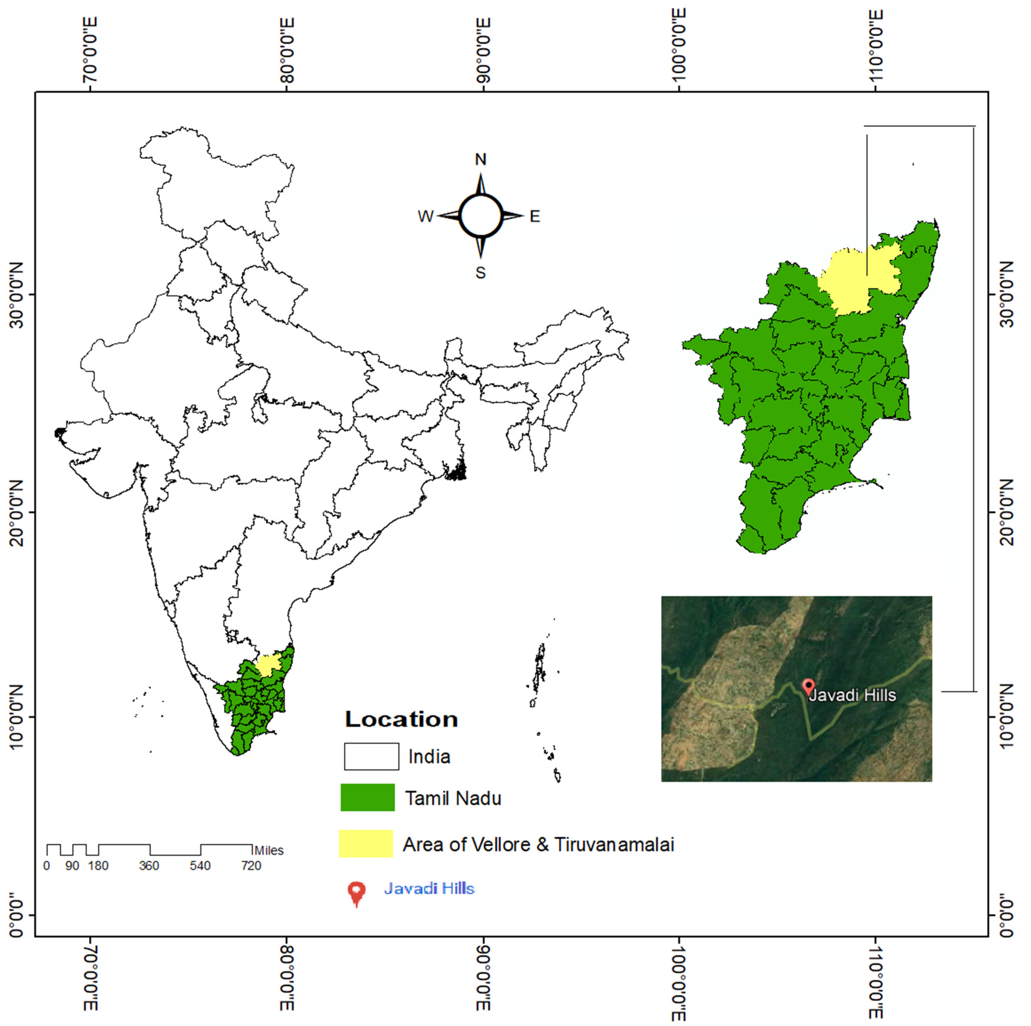
3.1. Study Area and Data Acquisition

The study area in our research work is the forest- and non-forest-covered area of Javadi Hills with the geographic coordinates falling between 78.75 E 12.5 N and 79.0 E 12.75 N. Our study area is located across the Eastern Ghats of Vellore and Tiruvannamalai district, Tamil Nadu, India. The UTM (Universal Transverse Mercator) GCS (geographic coordinate system)/WGS (World Geodetic System) 1984 (44 N) projection system was processed for the extracted satellite data. The location of the Javadi Hills map was extracted from Google Earth Engine (https://www.google.com/earth/ (accessed on 10 November 2021)). The map view of our study area was prepared by using ArcGIS (Version 10.1 developed by ESRI (http://www.esri.com/software/arcgis)) geospatial software, and it is shown in Figure 1.

The multispectral LISS-III satellite images for the years 2012 and 2015 were collected from the Bhuvan Indian Geo-Platform of ISRO (www.bhuvan.com (accessed on 9 December 2019)). The extracted LISS-III multispectral data of Javadi Hills were used for the LU/LC classification process. The TIRS, RED, and NIR bands of Landsat 8 (Band 10) and Landsat 7 (Band 6) were collected from the United States Geological Survey (USGS), United States (https://earthexplorer.usgs.gov (accessed on 16 December 2019)) and were used for the estimation of LST. There was no TIRS Band in the LISS-III sensor, so we extracted the TIRS image from the Landsat Satellite data for our study area. The importance of the TIRS band used in our paper provides the impact of LST on Javadi Hills for the years 2012 and 2015.

Table 1. Characteristics and sources of the satellite images.

Satellite	Path	Sensor	Year	Source
Resourcesat-1/2	101/064	LISS-III	18 February 2012 22 March 2015	Bhuvan Indian Geo-Platform of ISRO (www.bhuvan.com (accessed on 9 December 2019))
Landsat 8 OLI/TI and Landsat 7 (ETM+)	143/51	Operational Land Imager (OLI) and the Thermal Infrared (TI) Sensor	27 March 2015	United States Geological Survey (https://earthexplorer.usgs.gov (accessed on 16 December 2019))
		Enhanced Thematic Mapper Plus (ETM+)	26 March 2012

shows the source and characteristics of the remotely sensed satellite images. In our research work, the atmospheric corrections were made to provide good visibility to the extracted LISS-III multispectral satellite image of Javadi Hills. The scan-line error correction was made for filling the gaps in the extracted Landsat TIRS image of Javadi Hills. The geometric correction was made to extract the Region of Interest (ROI) coordinates in the forest- and non-forest-covered area of Javadi Hills that falls between 78.80 E 12.56 N and 78.85 E 12.60 N. Figure 2 represents the preprocessed image of multispectral LISS-III data of Javadi Hills for the years 2012 and 2015. Figure 3, Figure 4 and Figure 5 represent the preprocessed Landsat TIRS, RED, and NIR bands of the Javadi Hills for the years 2012 and 2015.

3.2. Proposed Vision Transformer Model for LU/LC Classification

A transformer is a deep-learning model that has emerged through the self-attention mechanism. The transformer follows the encoder–decoder architecture by processing the sequential data parallelly without depending on any recurrent network. It has been widely used in the scientific fields of NLP and computer vision. The Vision Transformer architecture has attracted an interesting view from researchers in recent years by showing good performance in the area of machine- and deep-learning applications. The Vision Transformer has been used in the area of image classification for providing state-of-the-art performance and to outperform the standard classification models. The Vision Transformer develops the encoder module of the transformer for performing the image classification by representing the sequence of image patches to the classified label. The attention mechanism of the Vision Transformer goes through all areas of the image and integrates the information into the full-sized image [47,48,49,50,51]. The end-to-end Vision Transformer model for the classification of satellite images is shown in Figure 6. The Vision Transformer classification model has experimented with the preprocessed LISS-III satellite image of Javadi Hills for the years 2012 and 2015. The Vision Transformer architecture is composed of an embedding, encoder, and classifier layer. Equations (1) and (2) represent the first step of analyzing and dividing the training images into a sequence of patches.

Let $S_i$ represent a set of training satellite images, $r$, where $X_i$ is a satellite image; $y_i$ represents the class labels $\left\{y_i\in 1, 2, \dots \dots , m\right\}$ associated with the $X_i$, and m denotes the number of defined LU/LC classes for that set.

$$S_i={\left\{X_i,y_i\right\}}_{i=1}^r$$

(1)

In the first step of the Vision Transformer model, an image $X_i$ from the training, the set is divided into non-overlapping patches of fixed size. Each patch is observed by the Vision Transformer as an individual token. Thus, from the size $h \ast w \ast c$(where $h$ is the height, $c$ is the number of channels, and $w$ is the width) of an image $X_i$, we extracted the patches of dimension $c \ast p \ast p$ ($p$ is the patch size) from it. The extracted patches are converted to a sequence of images $\left(x_1, x_2, x_3, \dots \dots \dots , x_n\right)$ of length $n$ through flattening.

$$n=hw/p^2$$

(2)

The image patches are linearly projected into a vector setup of model dimension, $d$, using the known embedding matrix, $E$. The concatenation of embedded representations is processed along with the trained classification token $vclass$ for performing the classification task. The positional information, $E_{pos}$, is programmed and attached to the patch representation. The spatial arrangements of the trained image patches were processed through positional embedding. The resulting sequence of image patches from positional embedding with token $z_0$ is given in Equation (3).

$$z_0=\left[vclass;x1E;x2E;\dots \dots \dots ,xnE\right]+E_{pos}, E\in {ℝ}^{\left(p^{2}c\right) \ast d}, E_{pos}\in {ℝ}^{\left(n+1\right) \ast d}$$

(3)

The resulting sequence of embedded image patches, $z_0$, is passed into the transformer encoder with $L$ identical layers. It has a multi-head self-attention block (MSA) and fully connected feed-forward MLP (Multilayer Perceptron) block with the GeLU activation function between them. The two subcomponents of the encoder work with the residual skip connections through the normalization layer $\left(LN\right)$. The representation of the two main components of the encoder is given in Equations (4) and (5). The last layer of the encoder, the first element in the sequence $z_L^0$, is passed into the head classifier for attaining the LU/LC classified classes.

$$z_l^1=MSA \left(LN\left(z_{l-1}\right)\right)+z_{l-1}, l=1\dots ..L$$

(4)

$$z_l=MLP \left(LN\left(z_l^1\right)\right)+z_l^1, l=1\dots ..L$$

(5)

$$y_i=LN \left(z_L^0\right)$$

(6)

The transformer block for the classification model is shown in Figure 7. The MSA block of the encoder is considered the central component of the transformer. The MSA block determines the importance of a single patch embedding with the other embeddings in the sequence. There are four layers in the MSA block: the linear layer, the self-attention layer, the concatenation layer, and a final linear layer. The attention weight is computed by calculating the weighted sum of all values in the sequence. The query-key-value scaling dot product is computed by the self-attention (SA) head through the attention weights The Q (query), K (key), and V (value) were generated by multiplying the element against three learned matrices $U_{QKV}$ (Equation (7)). For determining the significance of the elements on the sequence, the dot product is used between the Q vectors of one element with the K vectors of the other elements. The results show the importance of the image patches in the sequence. The outcomes of the dot product were scaled and passed into a Softmax (Equation (8)).

$$\left[\mathrm{Q},\mathrm{K},\mathrm{V}\right]=z{U}_{QKV}, U_{QKV}\in {ℝ}^{d \ast 3D_k}$$

(7)

$$A=softmax \left(\frac{Q{K}^T}{\sqrt{D_K}}\right), A\in {ℝ}^{n \ast n}$$

(8)

$$SA \left(z\right)=A.V$$

(9)

$$MSA \left(z\right)=Concat\left(S{A}_1\left(z\right); S{A}_2\left(z\right);\dots . S{A}_h\left(z\right)\right)W, W\in {ℝ}^{h.D_K \ast D}$$

(10)

The scaling-dot-product process achieved by the SA block is related to the standard dot product, but it includes the dimension of the key $D_K$ as a scaling factor. The patches with the high attention scores (Equation (8)) are processed by multiplying the outputs of Softmax with the values of each patch embedding vector. The results of all the attention heads are concatenated and provided to the MLP classifier for attaining the pixel value representation of the feature map (Equation (10)). The resampling was performed for adjusting the size of the feature map so that the output classified image would be represented in the standardized form during the time of accuracy assessment. The training data with different parameters that define the Vision Transformer classification model of our research work are presented in Section 5.1. The LU/LC classification map for the years 2012 and 2015 is shown in Figure 8. The accuracy assessment for the feature-extraction-based classification model is shown in Section 5.2. The evaluation of the LU/LC classification map was achieved through the accuracy assessment. The percentage of the LU/LC change between the years 2012 and 2015 for our study area was calculated. Based on the good accuracy results, the LU/LC change classification map was processed for further findings of the LU/LC prediction map.

3.3. Land Surface Temperature

The LST measures the skin temperature of the spatial data in the field of remote sensing. It displays the cold and hot temperature of the earth’s surface through the radiant energy reflected within the surface. The thermal-infrared remote-sensing data are used for measuring the LST. The TIRS data help in recognizing the mixture of bare soil and vegetation temperatures through LST [52,53,54]. In our research work, we estimated the LST for the TIRS bands of Landsat 8. Equations (11)–(13) represent the estimation of LST for TIRS image 7. The conversion of the Digital Number (DN) value to the radiance of the TIRS image is calculated by using Equation (11). The conversion of radiance into the brightness temperature is shown in Equation (12). The degree conversion from Kelvin (K) to Celsius © is shown in Equation (13).

$$L_{\lambda }=\left(\frac{LMA{X}_{\lambda }-LMI{N}_{\lambda }}{QCALMAX-QCALMIN}\right) \ast \left(QCAL-QCALMIN\right)+LMI{N}_{\lambda }$$

(11)

where $L_{\lambda }$ represents the spectral radiance in $\left(Watts/(m^2 \ast s{r}^2 \ast \mu m\right))$, $QCAL$ represents the quantized calibrated pixel value, $QCALMAX$ represents the maximum quantized calibrated pixel value, $QCALMIN$ represents the minimum quantized calibrated pixel value, $LMA{X}_{\mathsf{\lambda }}$ represents the spectral radiance scaled to $QCALMAX$, and $LMI{N}_{\mathsf{\lambda }}$ represents the spectral radiance scaled to $QCALMIN$.

$$T_K=\frac{K2}{\ln \left(\frac{K1}{L_{\lambda }}+1\right)}$$

(12)

$$C=T_K-273.15$$

(13)

where $T_{K }$ represents the effectiveness at the satellite temperature in Kelvin, and $K1 \mathrm{and} K2$ represent the calibration constants 1 and 2 in $\left(Watts/(m^2 \ast s{r}^2 \ast \mu m\right))$, respectively. For Landsat 7, the calibration constant value of $K1 \mathrm{and} K2$ is 666.09 and 1282.71, respectively.

Equations (14)–(20) represent the estimation of LST for the TIRS image of Landsat 8. By using the radiance rescaling factor, the conversion of Top of Atmosphere (TOA) spectral radiance is shown in Equation (14). By using the thermal infrared constant values in the metadata file of the satellite image, the spectral radiance data are converted to the TOA brightness temperature, and the expression is shown in Equation (15). The NDVI is calculated for differentiating the near-infrared and visible reflectance of the vegetation cover of the satellite data. The expression for NDVI is shown in Equation (16). The Land Surface Emissivity (LSE) is derived from NDVI values for displaying the average emissivity of the earth’s surface. The expressions are shown in Equations (17) and (18). By using the results of TOA brightness temperature, emitted radiance wavelength, and LSE, the LST was calculated and is shown in Equation (19).

$$T{L}_{\mathsf{\lambda }}=ML \ast QCAL+AL-O_i$$

(14)

where $T{L}_{\mathsf{\lambda }}$ represents the TOA spectral radiance in $\left(Watts/(m^2 \ast s{r}^2 \ast \mu m\right))$, $ML$ represents the radiance multiplicative band rescaling factor of the TIRS image, $QCAL$ represents the quantized calibrated pixel value, $AL$ represents the radiance additive band rescaling factor of TIRS image, and $O_i$ represents the correction value of the TIRS band of Landsat 8.

$$B{T}_P=\frac{K2}{\ln \left(\frac{K1}{T{L}_{\mathsf{\lambda }}}+1\right)}-273.15$$

(15)

where $B{T}_P$ represents TOA brightness temperature in Celsius, and $K1 \mathrm{and} K2$ represent the calibration constant 1 and 2 in $\left(Watts/(m^2 \ast s{r}^2 \ast \mu m\right))$, respectively. For Landsat 8, the calibration constant value of $K1 \mathrm{and} K2$ is 774.8853 and 1321.0789, respectively.

$$NDVI=\frac{\left(NIR-RED\right)}{\left(NIR+RED\right)}$$

(16)

where $NDVI$ represents the Normalized Difference Vegetation Index, $NIR$ represents the reflectance values of the near-infrared band, and $RED$ represents the reflectance values of the red band.

$$PV={\left(\left(NDVI-NDV{I}_{min}\right)/\left(NDV{I}_{max} – NDV{I}_{min}\right)\right)}^2$$

(17)

$$E=0.004 \ast PV+0.986$$

(18)

where $E$ represents the Land Surface Emissivity, $PV$ represents the Proportion of Vegetation, $NDVI$ represents the reflectance values of the $NDVI$ image, $NDV{I}_{max}$ represents the maximum reflectance value of the $NDVI$ image, and $NDV{I}_{min}$ represents the minimum reflectance value of the $NDVI$ image.

$$LST=\frac{B{T}_P}{\left(1+\left(\raisebox{1ex}{$\mathsf{\lambda } \ast B{T}_P$}\!\left/ \!\raisebox{-1ex}{$c2$}\right.\right) \ast \ln \left(E\right)\right)}$$

(19)

$$c2=\raisebox{1ex}{$pk \ast vl$}\!\left/ \!\raisebox{-1ex}{$bc$}\right.$$

(20)

where $LST$ represents Land Surface Temperature, $B{T}_P$ represents the TOA brightness temperature in Celsius ©, $\mathsf{\lambda }$ represents the wavelength of the emitted radiance, $pk$ represents the Planck’s constant value of $6.626 \ast {10}^{-34}\mathrm{J}\mathrm{s}$, $vl$ represents the velocity of the light value of $2.998\ast 108\mathrm{m}/\mathrm{s}$, and $bc$ represents the Boltzmann constant value of $1.38\ast {10}^{-34}\mathrm{JK}$. The statistical modeling of TIRS bands present in the Landsat satellite image was used for analyzing the LU/LC surface temperature of Javadi Hills, and it helps in improving the performance of the LU/LC prediction model. The LST map of Javadi Hills during the years 2012 and 2015 was analyzed by using the TIRS bands of Landsat 7 and 8 for the area of Javadi Hills. The flow of the calculation of LST for our area of Javadi Hills is shown in Figure 9. The LST map for the years 2012 and 2015 is shown in Figure 10. In this research work, we used the spatial features of the LST map and the LU/LC change classification map for evaluating the LU/LC prediction map for Javadi Hills. The LST map shows the features of the high- and low-temperature values of the earth’s surface. The high-temperature values indicate less vegetation, and the low-temperature value indicates a high-vegetation area. The impact of the LST map over the LU/LC change classification map provides good accuracy during the process of LU/LC prediction. The relationship between the values of the LST and LU/LC map is shown in Section 5.1.

3.4. Bidirectional Long Short-Term Memory Model for LU/LC Prediction

The LSTM model is considered the advanced model of RNN, where the long-term dependencies can be learned for the sequence prediction problems. The long-term vanishing-gradient problems are prevented by using the LSTM models. The key elements of the LSTM model are input, forget, and output gate [55,56,57]. Figure 11 displays the working principle of the LSTM model. In Figure 11, the vector operations represent the element-wise multiplication $(\ast ),$ and element-wise summation $(+)$ respectively. The time step (t) indicates the length of the input sequence in all the Equations (21)–(26). Equation (21) shows the mathematical expression of the forget gate, where $f_t$ represents the memory gate’s output at time t, $\sigma$ represents the sigmoid function (0 <$\sigma$ < 1), $W_f$ represents the weight value of ANN, $h_{t-1}$ is the output value of the previous cell, $x_t$ represents the input values, and $b_f$ denotes the bias weight values of the ANN. At the output of the equation, the value 1 will keep the information and the value 0 will forget the information

$$f_t=\sigma \left(W_f \ast \left[h_{t-1},x_t\right]+b_f\right)$$

(21)

$$I_t=\sigma \left(W_i \ast \left[h_{t-1},x_t\right]+b_i\right)$$

(22)

$$\widetilde{c_t}=tanh\left(W_c \ast \left[h_{t-1},x_t\right]+b_c\right)$$

(23)

In Equation (22), $I_t$ represents the output of the input gate, σ represents the sigmoid function, $W_i$ represents the weight values stored in the memory of ANN,$h_{t-1}$ is the output value of the previous cell, $x_t$ represents the input values, and $b_i$ denotes the bias weight values of the ANN.

In Equation (23), $\widetilde{c_t}$ represents the output of ANN with the normalized $tanh$ function that outputs the value between −1 and +1, $W_c$ represents the weight values stored in the memory of ANN, $h_{t-1}$ is the output value of the previous cell, $x_t$ represents the input values, and $b_c$ denotes the bias weight values of the ANN.

$$C_t=C_{t-1} \ast f_t+i_t \ast \widetilde{c_t}$$

(24)

$$O_t=\sigma \left(W_O \ast \left[h_{t-1},x_t\right]+b_O\right)$$

(25)

$$h_t=O_t\ast tanh \left(C_t\right)$$

(26)

Equation (24) shows the mathematical expression of the updated gate, where the memory is updated. The ANN learns the stored or forgotten information from the memory and then updates the newly added information from Equations (21)–(23). Equation (25) shows the mathematical expression of the output gate, where $W_O$ represents the weight values stored in the memory of ANN, $h_{t-1}$ is the output value of the previous cell, $x_t$ represents the input values, and $b_O$ denotes the bias weight values of the ANN. The output value, $h_t$, was calculated in Equation (26).

The uniform LU/LC classes were generated through the Vision Transformer classification model, and the features of the LST map were extracted for the years 2012 and 2015. In this research work, we used the spatial features of the LST map and the LU/LC change classification map for evaluating the LU/LC prediction map, using the Bi-LSTM model. The idea of Bi-LSTM is to process the sequence data in both forward and backward directions. The Bi-LSTM algorithm was used in our research for extracting the spatial and temporal features of the fifteen-year time-series data from 2012 to 2027 for the area of Javadi Hills. Figure 12 displays the working principle of the Bi-LSTM prediction model.

The inputs of the Bi-LSTM are given as the 3D vectors (samples, time steps, and features) for producing both spatial and temporal information. The samples define the number of the input LU/LC map ($L (j_{m,n}$)) of size ($m\ast n$) with defined labels $\left(j\right)$ for training and validation. With the LU/LC and LST features for the years 2012 and 2015, we have predicted and simulated the LU/LC map for the years 2018 and 2021. With the inputs of 2012 ($t-3)$, 2015 $\left(t\right)$, 2018 ($t+3)$, and 2021 $\left(t+6\right)$, the Bi-LSTM was processed in forward and backward directions for analyzing the features of time-series data and to project the predicted maps for the years 2021 $\left(t+9\right)$ and 2024 $\left(t+12\right)$ successfully. The features ($LC(j_{m,n}$)) define the LU/LC classes with the LST temperature values for each time step at defined coordinates. The input set of combined features of the LU/LC and LST map from the Javadi Hills was split by the ratio of 8:2 for the training and validation of the model. The parameters were adjusted through a trial-and-error approach for acquiring good prediction accuracy. The tanh activation function was used for the Bi-LSTM layers, whereas the Softmax activation functions were used for the last layer to calculate the probabilities between the LU/LC classes of Javadi Hills. Through repeated forward and back-propagation processes, the parameters are adjusted until the cost function is minimized. The validation method is part of training the prediction model and adjusting the parameters, which uses a small portion of data to validate and update the model parameters for each training epoch. The significant approach is to ensure that the prediction model is learning from data correctly by minimizing the cost function during the training and validation process. The training data with the parameters that run the Bi-LSTM prediction model for our research work are presented in Section 5.1. The LU/LC prediction map for the years 2018, 2021, 2024, and 2027 is shown in Figure 13 and Figure 14. The validation results of the LU/LC prediction model are shown in Section 5.2. Our proposed model provides good validation accuracy, and the growth patterns of the LU/LC results are shown in Section 5.3.

3.5. Application-Based Explainable Artificial Intelligence and Its Importance

The XAI provides knowledge to humans about the outcomes achieved by machine- or deep-learning models. The XAI has been used for providing knowledge on the extracted time-series LU/LC information to the urban planners, forest department, and government officials. XAI improves the user’s understanding and trust in the products or services. There are many ways of explaining the model through XAI, and the techniques of explaining the model differ for each application area around the world [58,59,60]. In our research work, we used application-based XAI, and it was observed to be the easiest and fastest way of obtaining knowledge with finite compute resources. The knowledge about the outcomes of the prediction model can be accessed through online applications. Technically, the application-based XAI can be understood by the end-users through third-party applications. In our prediction model, we used the Google Earth Engine (https://www.google.com/earth/ (accessed on 10 November 2021)) platform for explaining our results to urban planners, forest departments, and government officials. The LU/LC predicted results for the years 2018 and 2021 were tested through the Google Earth Engine time-series image. We achieved good testing accuracy for our prediction model. Through the XAI of the Google Earth Engine platform, the end-users can also access and check the LU/LC information. We have shown the model structure of XAI through the Google Earth Engine platform for our research work in Figure 15. The XAI on Google Earth will convey the LU/LC information to the government, forest department, and urban planners to take action in regard to protecting the LU/LC area.

4. Proposed LU/LC Prediction Using Vision Transformer–Based Bi-LSTM Model

This research work aimed to identify the LU/LC changes in the forest-covered (high vegetation) and non-forest-covered (less vegetation) regions of the proposed study area. The flow of LU/LC change for our study area is shown in Figure 16. The proposed flow of this work is described in the following steps,

• The LISS III satellite images for the years 2012 and 2015 of Javadi Hills, India, were collected from Bhuvan-Thematic Services of the National Remote Sensing Centre (NRSC), Indian Space Research Organization (ISRO).
• The Landsat satellite images for the years 2012 and 2015 of Javadi Hills, India, were collected from the United States Geological Survey (USGS), United States.
• Atmospheric, geometric, and radiometric corrections were performed to provide better visibility in the acquired LISS-III and Landsat images.
• The proposed Vision Transformers for classifying LU/LC classes were successfully performed for the years 2012 and 2015 of the LISS-III image.
• An LST map was calculated for the years 2012 and 2015 from Landsat TIRS images for extracting the spatial features.
• The relationship between the spatial features of the LST map with the LU/LC classification map were used to provide good validation results during the prediction process.
• The Bi-LSTM model was successfully applied to forecast the future LU/LC changes of Javadi Hills for the years 2018, 2021, 2024, and 2027.
• The LU/LC changes that occurred in our study area will assist the urban planners and forest department to take proper actions in the protection of the environment through XAI.

Algorithm to Construct the Vision Transformer–Based Bi-LSTM Model for LU/LC Prediction

Our research is based on the Vision Transformer–based Bi-LSTM model for LU/LC Prediction of Javadi Hills, India. From the brief analysis and validation, we found that the impact of the TIRS LST map with the LU/LC classified provides a good percentage of results with a lower misclassification rate. The detailed steps of our proposed model are presented in Algorithm 1. Each process in our proposed algorithm provides the different aspects of LU/LC information of Javadi Hills. A brief explanation of the input data, training data, parameter settings, and accuracy assessment of our proposed model is explained in Section 5.

Algorithm 1: To Construct the Vision Transformer–Based Bi-LSTM Prediction Model.

Inputs ($I_P$): The LISS-III multispectral satellite images for the years 2012 and 2015 (I1, I2), and Landsat bands for the years 2012 and 2015 $\left(I{R}_{1, }I{R}_2\right)$

Output ($O_P$): Predicted LU/LC images 2018, 2021, 2024, and 2027 $\left(P{R}_{1, } P{R}_{2 }, P{R}_{3 }, P{R}_{4 }\right)$

Begin

1  Input data ($I_P$):

2  Initialize the input data

3    Extract LISS-III multispectral image ($M=I_{1, }{I}_2$)

4    Extract Landsat bands $\left(T=I{R}_{1, }I{R}_2\right)$

5  Return input data ($I_P$)

6

7  Preprocessed data $\left(P{R}_I\right)$:

8  Initialize the input data for performing the preprocessing for the input data $I_P$ of M and T

9  For each initialized input image of M and T

10    Calculate the geometric coordinates of the study area $G_I$ (georeferencing)

11    Reduce the atmospheric (haze) effects $A_I$ of the georeferenced image

12    Correct the radiometric errors $R_I$ for the haze-reduced image

13  End for

14  Return preprocessed data $\left(P{R}_I\right)$

15

16  LU/LC classification ($L{U}_I$):

17  Perform the Vision Transformer–based LU/LC classification by using the preprocessed image $P{R}_I$

18  For each input image of $P{R}_I$

19    Load the training data $Ti$ and initialize the parameters

20    Split an image into patches of fixed size

21    Flatten the image patches

22    Perform the linear projection from the flattened patches

23    Include the positional embeddings

24    Feed the sequences as an input to the transformer encoder

25    Fine-tune the multi-head self-attention block in the encoder

26    Concatenate all the outputs of attention heads and provide the MLP classifier for attaining the pixel value representation of the feature map.

27    Generate the LU/LC classification map

28  End for

29  LU/LC classification ($L{U}_I$)

30

31  Accuracy assessment ($A{A}_I$):

32  Perform the accuracy assessment for the feature extraction–based LU/LC classification map $L{U}_I$

33  For each classified map of $L{U}_I$

34    Compare the labels of each classified data $L{U}_I$ with the Google Earth data

35    Build the confusion matrix

36    Calculate overall accuracy, precision, recall, and F1-Score

37    Summarize the performance of the classified map $L{U}_I$

38  End for

39  Return accuracy assessment $\left(A{A}_I\right)$

40

41  Change detection ($C{D}_I$):

42  Perform the LU/LC change detection by using the time-series LU/LC change classification map ($L{U}_I$)

43  For each classified map of $L{U}_I$

44  Calculate the percentage of change between the time-series classified map of $L{U}_I$

45  End For

46  Return change detection ($C{D}_I$)

47

48  Extracting LST map (LST)

49  Initialize the $I_P$ of T

50  For each preprocessed image of T

51    Calculate Land Surface Temperature using the Landsat bands (TIRS, RED, and NIR)

52    Extract the spatial features

53  End for

54  Return LST ($LS{T}_I$)

55

56  LU/LC prediction ($L{P}_I$):

57  Perform the Bi-LSTM prediction model by using the time-series LU/LC classification map of 2012 ($L{U}_1$) and 2015 ($L{U}_2$) and the spatial features of the LST map of 2012 ($LS{T}_1$) and 2015 ($LS{T}_2$)

58  For each time-series, LU/LC classified map of $L{U}_I$: {$L{U}_1, L{U}_2$} and LST map $LS{T}_I$: $\left\{LS{T}_1,LS{T}_2\right\}$

59  Perform LU/LC prediction $(L{P}_I)$ using Bi-LSTM model

60    Initialize the inputs for LU/LC prediction

61    Input $\left(IP\right)=\left\{L_1, LS{T}_1, L_2, LS{T}_2, \dots \right\}$

62    Combine the information of the time-series LU/LC classified map $L{U}_I$ with the LST map $LS{T}_I$

63    Load the 3D input vectors {samples, time steps, features}

64    Initialize the Bi-LSTM parameters

65    Apply tanh activation function for each Bi-LSTM layer

66    The output layer is decided by using the Softmax activation function

67    Update the parameters until the loss function is minimized

68    The output of the predicted time-series data is obtained

69    Validate the results

70  End for

71  Return LU/LC prediction map $L{P}_I$ $\left\{P{R}_{1, } P{R}_{2 }, \dots \right\}$

72  Analyze the growth patterns of the LU/LC prediction maps

73

74  Explain predicted results to the urban planners, forest department, and government officials, using application-based XAI

End

5. Results and Discussion

The problematic study on LU/LC prediction in Javadi was presented in this research work. The LISS-III multispectral, Landsat TIRS, RED, and NIR satellite images were used for predicting the vegetation in the forest- and non-forest-covered regions of the Javadi Hills. All the research experiments were processed on the Intel Xeon processor 2.90 GHz CPU, along with 128 GB RAM in Windows 10 (64-bit) environment. The needed libraries and packages of Python of version 3.10.2 developed by Python Software Foundation (https://www.python.org/) were installed for implementing the proposed model of our research. The backend geospatial software such as QGIS of version 3.6.1 developed by QGIS Development Team (https://qgis.org/en/site/), ArcGIS of version 10.1 developed by ESRI (http://www.esri.com/software/arcgis) and Google Earth Engine developed by Google (https://www.google.com/earth/) was used for preparing and analyzing the satellite data.

5.1. Training Data and Parameter Settings

For appropriate mapping of the input features to the output features using machine-learning or a deep-learning model, the training data and its parameters were used and tuned. Algorithm 1 shows the detailed procedure of our research on LU/LC prediction. The multispectral input map ($M$) of our study area Javadi Hills for the year 2012 and 2015 was considered as ($I_{1, } I_2$). The preprocessed multispectral image was processed for the further processing of our model.

The training samples of an image are divided into patches. The 16 patches (size = 64 × 4) were extracted from the input training image (256 × 256), of which each patch contains the trained LU/LC classes (high and less vegetation). The training samples for the area of Javadi Hills were generated through the latitude and longitudinal coordinates of Javadi Hills manually through Google Earth image. For the input image of Javadi Hills for the years 2012 and 2015, the LU/LC classification was performed through the Vision Transformer model. The working process of the Vision Transformer model was explained in Section 3.2. For a better understanding of our training samples in the patched image, we show the trained patches of 1 and 16 in Figure 17. The hyper-parameters used during the training process of the Vision Transformer model are shown in

Table 2. Hyperparameters of the Vision Transformer model.

Hyperparameters	Value
Learning Rate	0.001
Weight Decay	0.0001
Batch Size	10
Number of epochs	100
Image size	256 × 256
Patch size	64
Patches per image	16
Number of heads	4
Transformer Layers	8
Activation Function	GeLU
Optimizer	Adam

. The output extracted at the end of the fully connected layer was used as the LU/LC classified map for further processing.

After the classification, each classified sample was tested through the referenced data of Google Earth images. The LU/LC classified image ($L{U}_I$) was tested through the referenced Google Earth image. Each reference datum was labeled according to the respective LU/LC classes of the Javadi Hills through Google Earth images. The LU/LC class considered in our research work includes the high- and less-vegetation regions of the forest- and non-forest-covered regions of Javadi Hills. For better understanding, we have shown the validation of the point shape file with the Google Earth images in Figure 18, and the class values associated with each coordinate of the trained image are shown in

Table 3. Training data values for the area of Javadi Hills.

Training Feature Value	Longitude	Latitude	Class Value	Class Label
1	78.829746	12.581815	1	High Vegetation
241	78.81025	12.58796	2	Less Vegetation
1785	78.818244	12.580221	2	Less Vegetation
733	78.849159	12.576782	1	High Vegetation
6640	78.81107	12.57028	2	Less Vegetation
6277	78.83463	12.576789	1	High Vegetation
12,354	78.851079	12.59151	1	High Vegetation
12,179	78.80721	12.58024	2	Less Vegetation
20,163	78.81167	12.5669	2	Less Vegetation
30,759	78.841932	12.59148	1	High Vegetation
24,465	78.840458	12.591477	1	High Vegetation
28,861	78.805977	12.580232	2	Less Vegetation
35,655	78.836129	12.591499	1	High Vegetation
33,638	78.812464	12.580187	2	Less Vegetation
63	78.81674	12.60167	1	Less Vegetation
39,388	78.81276	12.58634	2	Less Vegetation

. The accuracy assessment was calculated for the Vision Transformer model, and the results are shown in Section 5.2.

The percentage of LU/LC change detection was calculated for the LU/LC classified image, and the results are shown in Section 5.3. Based on the good accuracy, the LU/LC classification map was processed for further findings of the LU/LC prediction map. The LST map for the years 2012 and 2015 was calculated to extract the spatial features of Javadi Hills. The estimation of the LST map was explained in Section 3.3. The LST map shows the features of the high- and low-temperature values of the earth’s surface of Javadi Hills. The high-temperature values indicate less vegetation, and the low-temperature value indicates a high-vegetation area. The LST ($LS{T}_I$) and the LU/LC ($L{U}_I$) classification map was used as an input for predicting the LU/LC map of Javadi Hills. We combined the time-series features of LST and the LU/LC map of Javadi Hills. The impact of LST on the LU/LC map provides good results during the prediction process. For a better understanding, we show the impact of a few LST and LU/LC features in Figure 19, and we show the values in

Table 4. LST and LU/LC values for the area of Javadi Hills.

Feature Value	Longitude	Latitude	Class Value	Temperature Value	Class Label
1	78.82975	12.58182	1	32.183754	High Vegetation
241	78.81025	12.58796	2	37.755061	Less Vegetation
1785	78.81824	12.58022	2	37.755061	Less Vegetation
733	78.84916	12.57678	1	31.708773	High Vegetation
6640	78.81107	12.57028	2	34.998298	Less Vegetation
6277	78.83463	12.57679	1	31.708773	High Vegetation
12,354	78.85108	12.59151	1	30.273344	High Vegetation
12,179	78.80721	12.58024	2	38.20916	Less Vegetation
20,163	78.81167	12.5669	2	34.998298	Less Vegetation
30,759	78.84193	12.59148	1	32.607521	High Vegetation
24,465	78.84046	12.59148	1	32.183754	High Vegetation
28,861	78.80598	12.58023	2	38.20916	Less Vegetation
35,655	78.83613	12.5915	1	31.708773	High Vegetation
33,638	78.81246	12.58019	2	34.533323	Less Vegetation
63	78.81674	12.60167	2	36.842331	Less Vegetation
39,388	78.81276	12.58634	2	38.20916	Less Vegetation

. The impact on the LST and LU/LC map strengthens our proposed predicted model with good validation results.

From the input LU/LC and LST features of 2012 and 2015, we predicted the LU/LC map of 2018 by using the Bi-LSTM model with the tuning of different parameters. The validated result provides good accuracy for our proposed model. We used the inputs of the LU/LC map of 2012 and 2015, along with the predicted LU/LC map of 2018 for predicting the LU/LC map for the year 2021. The short-term prediction was performed till the year 2027 for our study area. The working process of the Bi-LSTM model was explained in Section 3.4. The parameter used during the training process of the Bi-LSTM model is shown in

Table 5. Hyperparameters for the Bi-LSTM model.

Parameter	Value
Input Image Format	Raster
Number of Training Samples	51,200
Activation Function	tanh, Softmax
Dropout	0.1, 0.25
Learning Rate	0.001
Optimizer	Adam
Loss Function	Categorical Cross Entropy
Hidden layers	20
Number of epochs	100
Batch Size	32

.

The combined features of the LU/LC and LST map were used as the training features during the process of the Bi-LSTM training. Each pixel value was identified through the latitude and longitudinal coordinates of Javadi Hills manually through the combined features of the LU/LC and LST map. Each pixel holds either high or less vegetation for its defined coordinate system. The few combined values were shown in Table 4. For better understanding, we show the combined features map in Figure 20. The accuracy results for the prediction model are shown in Section 5.2. The results were also cross-verified with the time-series Google Earth Engine for acquiring the validation accuracy of our model. With the impact of the LST map with the LU/LC map, good validation accuracy was obtained with a lower misclassification rate.

5.2. Validation of Vision Transformer–Based Bi-LSTM Model

The Google Earth images with the LU/LC classified images were evaluated for the examination of accuracy assessment. By using the time-series images of the Google Earth Engine, the accuracy assessment was calculated for the LU/LC classified image of Javadi Hills. All the pixel values of the LU/LC classified image were validated with the Google Earth images. A total of 1008 random training samples were loaded, and the confusion matrix was obtained during the process of accuracy assessment.

Table 6. LU/LC confusion matrix.

LU/LC Classification	Class	Reference Class
		2012		2015
		High Vegetation	Less Vegetation	High Vegetation	Less Vegetation
Actual Class	High Vegetation	694	4	689	6
	Less Vegetation	7	303	8	305

represents the confusion matrix for the years 2012 and 2015. The results of the accuracy assessment for the year 2012 are 0.9891, and for 2015, it is 0.9861.

Table 7. LU/LC accuracy assessment for the proposed Vision Transformer model.

LU/LC Classification	2012	2015
Overall Accuracy	0.9891	0.9861
Precision	0.9901	0.9885
Recall	0.9942	0.9913
F1-Score	0.9921	0.9898

represents the LU/LC accuracy assessment for the years 2012 and 2015.

The LU/LC prediction was performed, and the results were analyzed and processed. The total number of pixel values was sliced into training and validation sets in an 8:2 proportion. The accuracy values of the prediction method look good for the LU/LC map of 2018 and 2021. The result of the validation accuracy for the year 2018 is 0.9865, and for 2021, it is 0.9811. The results were also cross-verified with the time-series Google Earth Engine image of Javadi Hills for the years 2018 and 2021 for acquiring the testing accuracy of our model. The results of the testing accuracy for our model also provide good results for 2018 and 2021. The results of the testing accuracy for the year 2018 is 0.9696, and for 2021, it is 0.9673. The results of the testing and validation accuracy of the predicted map are presented in

Table 8. Validation and testing process of the proposed Vision Transformer–based Bi-LSTM Prediction Model.

Input Map (Year)	Training Feature Map (256 × 200 Pixels)	Train—Validation Split (8:2) Data	Test Data (Google Earth Image)	Predicted Map	Validation Accuracy	Testing Accuracy
LU/LC Classification—LST Map (2012, and 2015)	51,200	40,960–10,240	51,200	2018	0.9865	0.9696
	51,200	40,960–10,240	51,200	2021	0.9811	0.9673

. The validation accuracy refers to the results of the non-trained datasets of the model. The testing accuracy refers to the results of the complete model. We used the inputs of the LU/LC map of 2012 and 2015, along with the predicted LU/LC map of 2018 and 2021 for predicting the LU/LC map for the years 2024 and 2027. The short-term prediction was performed till the year 2027 for our study area. As the Google Earth Engine provides the time-series image till the current date, the validation and testing accuracy for the predicted LU/LC map of 2024 and 2027 was not calculated. With the results of the good validation accuracy for all the LU/LC predicted maps of Javadi Hills, our prediction model provides a lower misclassification rate.

$$Average Model Accuracy=\left(\frac{A_{Y1}+A_{Y2}+\dots +A_{Yn}}{\mathrm{T}}\right) \ast 100$$

(27)

where $A_Y$ represents the accuracy value of years $\left\{1\dots .n\right\}$, and $\mathrm{T}$ represents the total number of years. The importance of providing the performance of the model depends on the average classification and prediction results. The average classification and prediction accuracy for the time series LU/LC data have been calculated by using Equation (27). The accuracy results for the years 2012 (0.9891) and 2015 (0.9861) were used for providing the performance of the calculation model through the average model accuracy. The average classification accuracy that was obtained was 98.76% for the proposed Vision Transformer model. The validation and testing results of our prediction model for the year 2018 are 0.9865 and 0.9696, respectively. The validation and testing results of our prediction model for the year 2021 are 0.9811 and 0.9673, respectively. The average validation accuracy is 98.38%, and the testing accuracy is 96.84% for our prediction model. We infer that the impact of the LST spatial variable from TIRS bands with the classified LU/LC map provides a good percentage of results.

The computational complexity defines the total time taken by the computer for running an algorithm. The computational complexity of the Vision Transformer model is $O \left(nC\right)$, where $n$ is the size of input, and $C$ is the number of classified LU/LC classes. The computational complexity of the Bi-LSTM prediction model is $O \left(nkC+1\right)$, where $k$ is the size of the spatial maps (LST) associated with input data $n$. Hence, the total computational time of our proposed algorithm $C_c$ is the arithmetic sum of the classification and prediction model, which is given in Equation (28).

$$C_c=O \left(nC\right)+O \left(nkC+1\right)$$

(28)

Although the proposed Vision Transformer–based Bi-LSTM prediction model shows significant performance, its training phase requires the determination of class values associated with spatial maps for each pixel in the $n$ images, and this is computationally expensive.

5.3. Growth Pattern of the LU/LC Area of Javadi Hills

The growth patterns of LU/LC change in the area of Javadi Hills were performed between the years 2012 to 2027, and the results are shown in

Table 9. LU/LC area statistics for LU/LC Map (2012–2027).

LU/LC Class	Area (ha)
	Year
	2012	2015	2018	2021	2024	2027
High Vegetation	1651.04	1601.22	1621.18	1596.04	1568.23	1553.17
Less Vegetation	736.85	786.67	766.71	791.85	819.66	834.72
Total (ha)	2387.89	2387.89	2387.89	2387.89	2387.89	2387.89

. In 2012, the LU/LC multispectral classified map was found to be 1651.04 ha (hectare) of the high vegetation and 736.85 ha of less vegetation. In 2015, the LU/LC multispectral classified map was found to be 1601.22 ha of vegetation and 786.67 ha of less vegetation. In 2018, the LU/LC predicted map was found to be 1621.18 ha of high vegetation and 766.71 ha of less vegetation. In 2021, the LU/LC predicted map was found to be 1596.04 ha of high vegetation and 791.85 ha of less vegetation. In 2024, the LU/LC predicted map was found to be 1568.23 ha of high vegetation and 819.66 ha of less vegetation. In 2027, the LU/LC predicted map was found to be 1553.17 ha of high vegetation and 834.72 ha of less vegetation. It was observed that the LU/LC changes have been frequently happening every three years in the area of Javadi Hills. The results of the LU/LC change that occurred between the years 2012 to 2027 are shown in

Table 10. Percentage of LU/LC change for the area of Javadi Hills during 2012–2027.

LU/LC Class	Area (%)
	Year
	2012–2015	2015–2018	2018–2021	2021–2024	2024–2027
High Vegetation	−3.01	1.24	−1.55	−1.74	−0.96
Less Vegetation	6.76	−2.53	3.27	3.51	1.83

. The comparison chart of LU/LC area statistics for the time-series data from 2012 to 2027 is shown in Figure 21.

6. Comparative Analysis

In this research work, we have proposed the Vision Transformer–based Bi-LSTM prediction model for analyzing the past, present, and future changes of Javadi Hills, India. We also infer that the LU/LC prediction accuracy of our model provides a lower error rate, i.e., below 5%. From the thorough analysis, we infer that the use of the LST map has a high impact on the LU/LC environment, and it was considered an important spatial feature for the prediction of the LU/LC vegetation map.

We have compared our model with CNN, DWT, and standard LU/LC classification and prediction techniques for the area of Javadi Hills. Our model outperforms the other standard classification and prediction algorithms in terms of accuracy and computational efficiency. We have executed the standard LU/LC algorithms (DWT [22], CNN [27], SVM [1], MLC [2], and RFC [25]) and provided a comparative analysis of the Vision Transformer model for our study area of Javadi Hills in

Table 11. Comparative analysis of the proposed Vision Transformer model with other algorithms for the area of Javadi Hills, India.

Algorithms	Average Accuracy (%)
Ours	98.76
CNN [27]	96.42
DWT [22]	94.21
SVM [1]	97.71
MLC [2]	94.4
RFC [25]	95.6

. We have also presented the comparative accuracy of the classification model in Figure 22. We have also shown the comparative analysis of our prediction model with the hybrid machine-learning models [7] for the area of Javadi Hills in

Table 12. Comparative analysis of LU/LC prediction models for the area of Javadi Hills, India.

Study Area	Algorithm	Prediction Accuracy (%)
Javadi Hills, India	Vision Transformer–based Bi-LSTM Model (ours)	98.38%
	RFC-based MC–ANN–CA Model [7]	93.41%

.

Our model outperforms the hybrid machine-learning models [7] and provides good prediction accuracy. We have validated the use of the LST map with other spatial maps that include a slope, aspect, and distances from the road map [7] for our prediction model. From the thorough analysis, we infer that the use of the LST map has a high impact on the LU/LC environment, and it has been considered an important spatial feature for the prediction of the LU/LC vegetation map. We have shown a few comparisons of the validation results of the LU/LC prediction methods by using LST, slope, aspect, and distance from the road map for the area of Javadi Hills in

Table 13. Testing of the Vision Transformer–based Bi-LSTM model using the various combinations of Input Spatial Data for Javadi Hills, India.

Study Area	Input Data	Prediction Accuracy (%)
Javadi Hills, India	LU/LC Classification—LST Map	98.38
	LU/LC Classification—Slope Map	92.33
	LU/LC Classification—Distance from Road Map	91.64
	LU/LC Classification—Slope, Distance from road map	92.52
	LU/LC Classification—Slope, LST map	93.45
	LU/LC Classification—Distance from Road, LST map	93.17
	LU/LC Classification—Slope, Distance from Road, LST map	94.2

.

We also show a few comparative analyses of overall prediction models for a few different study areas in

Table 14. Comparative analysis of LU/LC prediction models for different study areas.

Study Area	Algorithm	Prediction Accuracy (%)
Javadi Hills, India (our study)	Vision Transformer–Based Bi-LSTM Model	98.38
Wuhan, China [28]	Self-Adaptive Cellular-Based Deep-Learning LSTM Model	93.1
Guangdong province of South China [23]	Deep Learning (RNN–CNN) and CA–MC Model	95.86
Western Fansu Province, China [26]	CNN–GRU Model	93.46
Dhaka, Bangladesh [29]	CA–MC and ANN Model	90.21
University of Nebraska–Lincoln [24]	CNN–Bi-LSTM Model	91.73
City of Surrey, British Columbia [56]	RNN–ConvLSTM Model	88.0
Klingenberg, Germany [55]	Fully CNN–LSTM Model	87.0
Awadh, Lucknow [6]	CA–MC and LR model	84.0

. We observed that there is a performance variation in the prediction results for each study area around the world. This variation of the LU/LC classification and prediction results was due to the selection of study area, satellite data, environmental data, and its LU/LC classes. A variation of results was observed for our study area with the assessment of multi-satellite datasets through the proposed algorithm. We delivered a clear view of the importance of Vision Transformer–based LU/LC classification and Bi-LSTM-based prediction for forecasting the time series LU/LC vegetation map. The advantage of our proposed work lies in using only the LST map as the spatial data for predicting the LU/LC vegetation map. We also achieved a good prediction accuracy of 98.38%. Our proposed algorithm can be applied to other study areas around the world in predicting the LU/LC vegetation map. Moreover, our proposed model has been efficient for urban planners, forest departments, and government officials in analyzing the LU/LC information through XAI and taking necessary actions in the protection of the LU/LC environment.

7. Conclusions

The LU/LC prediction modeling was considered important research in the area of remote sensing. In this research work, the multispectral LISS-III and Landsat satellite image of Javadi Hills for the periods 2012 and 2015 were downloaded and performed for analyzing the LU/LC prediction for the years 2018, 2021, 2024, and 2027. The Vision Transformer model for performing the LU/LC classification was proposed, and the accuracy assessment was performed by using Google Earth Images. The average classification accuracy obtained for our Vision Transformer model was 98.76%. The spatial features from the LST map and LU/LC classified map were used as input for predicting the LU/LC changes in Javadi Hills. For predicting the future LU/LC changes of Javadi Hills, the Bi-LSTM model was successfully applied. We infer that the impact of the LST spatial features with the LU/LC classified map provides a good percentage of results with 98.38%. The predicted results provide the variation in the high- and less-vegetation regions of Javadi Hills from 2012 to 2027. Our Vision Transformer–based Bi-LSTM model has produced good validation results when compared with other standardized models. Our research on LU/LC prediction provides information to the forest departments, urban planners, and government officials to take necessary action in the protection of the LU/LC environment through application-based XAI. In the future, we plan to focus more on using the TIRS bands of hyperspectral data to obtain the temperature values associated with each pixel and to classify the hyperspectral data in real-time scenarios.

References

1. Baig, M.F.; Mustafa, M.R.U.; Baig, I.; Takaijudin, H.B.; Zeshan, M.T. Assessment of land use land cover changes and future predictions using CA-ANN simulation for selangor, Malaysia. Water 2022, 14, 402. [Google Scholar] [CrossRef]
2. Imran, M.; Aqsa, M. Analysis and mapping of present and future drivers of local urban climate using remote sensing: A case of Lahore, Pakistan. Arab. J. Geosci. 2020, 13, 1–14. [Google Scholar] [CrossRef]
3. Heidarlou, H.B.; Shafiei, A.B.; Erfanian, M.; Tayyebi, A.; Alijanpour, A. Effects of preservation policy on land use changes in Iranian Northern Zagros forests. Land Use Policy 2019, 81, 76–90. [Google Scholar] [CrossRef]
4. Chaves, M.E.D.; Michelle, C.A.P.; Ieda, D.S. Recent applications of Landsat 8/OLI and Sentinel-2/MSI for land use and land cover mapping: A systematic review. Remote Sens. 2020, 12, 3062. [Google Scholar] [CrossRef]
5. Priyadarshini, K.N.; Kumar, M.; Rahaman, S.A.; Nitheshnirmal, S. A comparative study of advanced land use/land cover classification algorithms using Sentinel-2 data. Int. Arch. Photogramm. Remote Sens. Spat. Inf. Sci. 2018, 42, 20–23. [Google Scholar] [CrossRef] [Green Version]
6. Siddiqui, A.; Siddiqui, A.; Maithani, S.; Jha, A.K.; Kumar, P.; Srivastav, S.K. Urban growth dynamics of an Indian metropolitan using CA markov and logistic regression. Egypt. J. Remote Sens. Space Sci. 2018, 21, 229–236. [Google Scholar] [CrossRef]
7. Mohan, R.; Sam, N.; Agilandeeswari, L. Modelling spatial drivers for LU/LC change prediction using hybrid machine learning methods in Javadi Hills, Tamil Nadu, India. J. Indian Soc. Remote Sens. 2021, 49, 913–934. [Google Scholar] [CrossRef]
8. Sandamali, S.P.I.; Lakshmi, N.K.; Sundaramoorthy, S. Remote sensing data and SLEUTH urban growth model: As decision support tools for urban planning. Chin. Geogr. Sci. 2018, 28, 274–286. [Google Scholar] [CrossRef] [Green Version]
9. Hegde, G.; Ahamed, J.M.; Hebbar, R.; Raj, U. Urban land cover classification using hyperspectral data. Int. Arch. Photogramm. Remote Sens. Spat. Inf. Sci. 2014, 8, 751–754. [Google Scholar] [CrossRef] [Green Version]
10. Elmore, A.J.; John, F.M. Precision and accuracy of EO-1 Advanced Land Imager (ALI) data for semiarid vegetation studies. IEEE Trans. Geosci. Remote Sens. 2003, 41, 1311–1320. [Google Scholar] [CrossRef]
11. Elbeih, S.F.; El-Zeiny Ahmed, M. Qualitative assessment of groundwater quality based on land use spectral retrieved indices: Case study Sohag Governorate, Egypt. Remote Sens. Appl. Soc. Environ. 2018, 10, 82–92. [Google Scholar] [CrossRef]
12. Nagy, A.; El-Zeiny, A.; Sowilem, M.; Atwa, W.; Elshaier, M. Mapping mosquito larval densities and assessing area vulnerable to diseases transmission in Nile valley of Giza, Egypt. Egypt. J. Remote Sens. Space Sci. 2022, 25, 63–71. [Google Scholar] [CrossRef]
13. Etemadi, H.; Smoak, J.M.; Karami, J. Land use change assessment in coastal mangrove forests of Iran utilizing satellite imagery and CA–Markov algorithms to monitor and predict future change. Environ. Earth Sci. 2018, 77, 1–13. [Google Scholar] [CrossRef]
14. Goodarzi Mehr, S.; Ahadnejad, V.; Abbaspour, R.A.; Hamzeh, M. Using the mixture-tuned matched filtering method for lithological mapping with Landsat TM5 images. Int. J. Remote Sens. 2013, 34, 8803–8816. [Google Scholar] [CrossRef]
15. Vijayan, D.; Shankar, G.R.; Shankar, T.R. Hyperspectral data for land use/land cover classification. Int. Arch. Photogramm. Remote Sens. Spat. Inf. Sci. 2014, 40, 991. [Google Scholar] [CrossRef] [Green Version]
16. Myint, S.W.; Okin, G.S. Modelling land-cover types using multiple endmember spectral mixture analysis in a desert city. Int. J. Remote Sens. 2009, 30, 2237–2257. [Google Scholar] [CrossRef]
17. Amigo, J.M.; Carolina, S. Preprocessing of hyperspectral and multispectral images. In Data Handling in Science and Technology; Elsevier: Amsterdam, The Netherlands, 2020; Volume 32, pp. 37–53. [Google Scholar] [CrossRef]
18. HongLei, Y.; JunHuan, P.; BaiRu, X.; DingXuan, Z. Remote sensing classification using fuzzy C-means clustering with spatial constraints based on Markov random field. Eur. J. Remote Sens. 2013, 46, 305–316. [Google Scholar] [CrossRef] [Green Version]
19. Navin, M.S.; Agilandeeswari, L. Comprehensive review on land use/land cover change classification in remote sensing. J. Spectr. Imaging 2020, 9, a8. [Google Scholar] [CrossRef]
20. Ganasri, B.P.; Dwarakish, G.S. Study of land use/land cover dynamics through classification algorithms for Harangi catchment area, Karnataka State, India. Aquat. Procedia 2015, 4, 1413–1420. [Google Scholar] [CrossRef]
21. Sharma, J.; Prasad, R.; Mishra, V.N.; Yadav, V.P.; Bala, R. Land use and land cover classification of multispectral LANDSAT-8 satellite imagery using discrete wavelet transform. Int. Arch. Photogramm. Remote Sens. Spat. Inf. Sci. 2018, 42, 703–706. [Google Scholar] [CrossRef] [Green Version]
22. Kabisch, N.; Selsam, P.; Kirsten, T.; Lausch, A.; Bumberger, J. A multi-sensor and multi-temporal remote sensing approach to detect land cover change dynamics in heterogeneous urban landscapes. Ecol. Indic. 2019, 99, 273–282. [Google Scholar] [CrossRef]
23. Xing, W.; Qian, Y.; Guan, X.; Yang, T.; Wu, H. A novel cellular automata model integrated with deep learning for dynamic spatio-temporal land use change simulation. Comput. Geosci. 2020, 137, 104430. [Google Scholar] [CrossRef]
24. Ali, A.S.A.; Ebrahimi, S.; Ashiq, M.M.; Alasta, M.S.; Azari, B. CNN-Bi LSTM neural network for simulating groundwater level. Environ. Eng. 2022, 8, 1–7. [Google Scholar] [CrossRef]
25. Floreano, I.X.; de Moraes, L.A.F. Land use/land cover (LULC) analysis (2009–2019) with google earth engine and 2030 prediction using Markov-CA in the Rondônia State, Brazil. Environ. Monit. Assess. 2021, 193, 1–17. [Google Scholar] [CrossRef]
26. Xiao, B.; Liu, J.; Jiao, J.; Li, Y.; Liu, X.; Zhu, W. Modeling dynamic land use changes in the eastern portion of the hexi corridor, China by cnn-gru hybrid model. GIScience Remote Sens. 2022, 59, 501–519. [Google Scholar] [CrossRef]
27. Gaetano, R.; Ienco, D.; Ose, K.; Cresson, R. A two-branch CNN architecture for land cover classification of PAN and MS imagery. Remote Sens. 2018, 10, 1746. [Google Scholar] [CrossRef] [Green Version]
28. Mu, L.; Wang, L.; Wang, Y.; Chen, X.; Han, W. Urban land use and land cover change prediction via self-adaptive cellular based deep learning with multisourced data. IEEE J. Sel. Top. Appl. Earth Obs. Remote Sens. 2019, 12, 5233–5247. [Google Scholar] [CrossRef]
29. Al Kafy, A.; Dey, N.N.; Al Rakib, A.; Rahaman, Z.A.; Nasher, N.R.; Bhatt, A. Modeling the relationship between land use/land cover and land surface temperature in Dhaka, Bangladesh using CA-ANN algorithm. Environ. Chall. 2021, 4, 100190. [Google Scholar] [CrossRef]
30. MohanRajan, S.N.; Loganathan, A.; Manoharan, P. Survey on land use/land cover (LU/LC) change analysis in remote sensing and GIS environment: Techniques and challenges. Environ. Sci. Pollut. Res. 2020, 27, 29900–29926. [Google Scholar] [CrossRef]
31. Dosovitskiy, A.; Beyer, L.; Kolesnikov, A.; Weissenborn, D.; Zhai, X.; Unterthiner, T.; Dehghani, M.; Minderer, M.; Heigold, G.; Gelly, S.; et al. An image is worth 16x16 words: Transformers for image recognition at scale. arXiv 2020, arXiv:2010.11929. [Google Scholar] [CrossRef]
32. Hong, D.; Han, Z.; Yao, J.; Gao, L.; Zhang, B.; Plaza, A.; Chanussot, J. SpectralFormer: Rethinking hyperspectral image classification with transformers. IEEE Trans. Geosci. Remote Sens. 2021, 60, 1–15. [Google Scholar] [CrossRef]
33. Wen, Q.; Zhou, T.; Zhang, C.; Chen, W.; Ma, Z.; Yan, J.; Sun, L. Transformers in time series: A survey. arXiv 2022, arXiv:2202.07125. [Google Scholar] [CrossRef]
34. Khan, S.; Naseer, M.; Hayat, M.; Zamir, S.W.; Khan, F.S.; Shah, M. Transformers in vision: A survey. ACM Comput. Surv. (CSUR) 2021, 1–38. [Google Scholar] [CrossRef]
35. Bazi, Y.; Bashmal, L.; Rahhal, M.M.A.; Dayil, R.A.; Ajlan, N.A. Vision transformers for remote sensing image classification. Remote Sens. 2021, 13, 516. [Google Scholar] [CrossRef]
36. Xu, K.; Deng, P.; Huang, H. Vision transformer: An excellent teacher for guiding small networks in remote sensing image scene classification. IEEE Trans. Geosci. Remote Sens. 2022, 60, 1–15. [Google Scholar] [CrossRef]
37. Sha, Z.; Li, J. MITformer: A multi-instance vision transformer for remote sensing scene classification. IEEE Geosci. Remote Sens. Lett. 2022, 19, 1–5. [Google Scholar] [CrossRef]
38. Xu, F.; Uszkoreit, H.; Du, Y.; Fan, W.; Zhao, D.; Zhu, J. Explainable AI: A brief survey on history, research areas, approaches and challenges. In CCF International Conference on Natural Language Processing and Chinese Computing; Tang, J., Kan, M.Y., Zhao, D., Li, S., Zan, H., Eds.; Springer: Cham, Switzerland, 2019. [Google Scholar] [CrossRef]
39. Schlegel, U.; Arnout, H.; El-Assady, M.; Oelke, D.; Keim, D.A. Towards a rigorous evaluation of XAI methods on time series. In Proceedings of the 2019 IEEE/CVF International Conference on Computer Vision Workshop (ICCVW), Seoul, Korea, 27–28 October 2019; IEEE: Manhattan, NY, USA, 2020. [Google Scholar] [CrossRef] [Green Version]
40. Saeed, W.; Christian, O. Explainable AI (XAI): A systematic meta-survey of current challenges and future opportunities. arXiv 2021, arXiv:2111.06420. [Google Scholar] [CrossRef]
41. Ribeiro, J.; Silva, R.; Cardoso, L.; Alves, R. Does dataset complexity matters for model explainers? In Proceedings of the 2021 IEEE International Conference on Big Data (Big Data), Orlando, FL, USA, 15–18 December 2021; IEEE: Manhattan, NY, USA, 2022. [Google Scholar] [CrossRef]
42. Samek, W.; Montavon, G.; Lapuschkin, S.; Anders, C.J.; Müller, K.R. Explaining deep neural networks and beyond: A review of methods and applications. IEEE 2021, 109, 247–278. [Google Scholar] [CrossRef]
43. LinarLinardatos, P.; Papastefanopoulos, V.; Kotsiantis, S. Explainable AI: A review of machine learning interpretability methods. Entropy 2020, 23, 18. [Google Scholar] [CrossRef]
44. Navin, M.S.; Agilandeeswari, L. Multispectral and hyperspectral images based land use/land cover change prediction analysis: An extensive review. Multimed. Tools Appl. 2020, 79, 29751–29774. [Google Scholar] [CrossRef]
45. Ma, L.; Liu, Y.; Zhang, X.; Ye, Y.; Yin, G.; Johnson, B.A. Deep learning in remote sensing applications: A meta-analysis and review. ISPRS J. Photogramm. Remote Sens. 2019, 152, 166–177. [Google Scholar] [CrossRef]
46. Thyagharajan, K.K.; Vignesh, T. Soft computing techniques for land use and land cover monitoring with multispectral remote sensing images: A review. Arch. Comput. Methods Eng. 2019, 26, 275–301. [Google Scholar] [CrossRef]
47. Kaselimi, M.; Voulodimos, A.; Daskalopoulos, I.; Doulamis, N.; Doulamis, A. A Vision transformer model for convolution-free multilabel classification of satellite imagery in deforestation monitoring. IEEE Trans. Neural Netw. Learn. Syst. 2022, 1–9. [Google Scholar] [CrossRef] [PubMed]
48. Liu, X.; Wu, Y.; Liang, W.; Cao, Y.; Li, M. High resolution SAR image classification using global-local network structure based on vision transformer and CNN. IEEE Geosci. Remote Sens. Lett. 2022, 19, 1–5. [Google Scholar] [CrossRef]
49. Ghali, R.; Akhloufi, M.A.; Jmal, M.; Souidene Mseddi, W.; Attia, R. Wildfire segmentation using deep vision transformers. Remote Sensing 2021, 13, 3527. [Google Scholar] [CrossRef]
50. Chen, X.; Qiu, C.; Guo, W.; Yu, A.; Tong, X.; Schmitt, M. Multiscale feature learning by transformer for building extraction from satellite images. IEEE Geosci. Remote Sens. Lett. 2022, 19, 1–5. [Google Scholar] [CrossRef]
51. Meng, X.; Wang, N.; Shao, F.; Li, S. Vision transformer for pansharpening. IEEE Trans. Geosci. Remote Sens. 2022, 60, 1–11. [Google Scholar] [CrossRef]
52. Mukherjee, F.; Singh, D. Assessing land use–land cover change and its impact on land surface temperature using LANDSAT data: A comparison of two urban areas in India. Earth Syst. Environ. 2020, 4, 385–407. [Google Scholar] [CrossRef]
53. Sekertekin, A.; Stefania, B. Land surface temperature retrieval from Landsat 5, 7, and 8 over rural areas: Assessment of different retrieval algorithms and emissivity models and toolbox implementation. Remote Sens. 2020, 12, 294. [Google Scholar] [CrossRef] [Green Version]
54. Nasir, M.J.; Ahmad, W.; Iqbal, J.; Ahmad, B.; Abdo, H.G.; Hamdi, R.; Bateni, S.M. Effect of the urban land use dynamics on land surface temperature: A case study of kohat city in Pakistan for the period 1998–2018. Earth Syst. Environ. 2022, 6, 237–248. [Google Scholar] [CrossRef]
55. Sefrin, O.; Riese, F.M.; Keller, S. Deep learning for land cover change detection. Remote Sens. 2020, 13, 78. [Google Scholar] [CrossRef]
56. Cao, C.; Dragićević, S.; Li, S. Short-term forecasting of land use change using recurrent neural network models. Sustainability 2019, 11, 5376. [Google Scholar] [CrossRef] [Green Version]
57. Wang, H.; Zhao, X.; Zhang, X.; Wu, D.; Du, X. Long time series land cover classification in China from 1982 to 2015 based on Bi-LSTM deep learning. Remote Sens. 2019, 11, 1639. [Google Scholar] [CrossRef] [Green Version]
58. Adadi, A.; Mohammed, B. Peeking inside the black-box: A survey on explainable artificial intelligence (XAI). IEEE Access 2018, 6, 52138–52160. [Google Scholar] [CrossRef]
59. Fulton, L.B.; Lee, J.Y.; Wang, Q.; Yuan, Z.; Hammer, J.; Perer, A. Getting playful with explainable AI: Games with a purpose to improve human understanding of AI. In Proceedings of the Extended Abstracts of the 2020 CHI Conference on Human Factors in Computing Systems, Honolulu, HI, USA, 25–30 April 2020; Association for Computing Machinery: New York, NY, USA, 2020. [Google Scholar] [CrossRef]
60. Kute, D.V.; Pradhan, B.; Shukla, N.; Alamri, A. Deep learning and explainable artificial intelligence techniques applied for detecting money laundering–a critical review. IEEE Access 2021, 9, 82300–82317. [Google Scholar] [CrossRef]
Figure 1. Study Area—Javadi Hills, India.
Applsci 12 06387 g001
Figure 2. Preprocessed LISS-III multispectral image of Javadi Hill for the years (a) 2012 and (b) 2015.
Applsci 12 06387 g002
Figure 3. Preprocessed Landsat TIRS bands of Javadi Hill for the years (a) 2012 and (b) 2015.
Applsci 12 06387 g003
Figure 4. Preprocessed Landsat RED bands of Javadi Hill for the years (a) 2012 and (b) 2015.
Applsci 12 06387 g004
Figure 5. Preprocessed Landsat NIR bands of Javadi Hill for the years (a) 2012 and (b) 2015.
Applsci 12 06387 g005
Figure 6. Proposed Vision Transformer model for LU/LC classification.
Applsci 12 06387 g006
Figure 7. Transformer block for the Vision Transformer classification model.
Applsci 12 06387 g007
Figure 8. LU/LC classification map of Javadi Hills for the years (a) 2012 and (b) 2015.
Applsci 12 06387 g008
Figure 9. The flow of Land Surface Temperature estimation for the area of Javadi Hills, India.
Applsci 12 06387 g009
Figure 10. LST map for the area of Javadi Hills for the years (a) 2012 and (b) 2015.
Applsci 12 06387 g010
Figure 11. LSTM model.
Applsci 12 06387 g011
Figure 12. Bi-LSTM model for LU/LC prediction.
Applsci 12 06387 g012
Figure 13. LU/LC prediction map of Javadi Hills for the years (a) 2018 and (b) 2021.
Applsci 12 06387 g013
Figure 14. LU/LC prediction map of Javadi Hills for the years (a) 2024 and (b) 2027.
Applsci 12 06387 g014
Figure 15. Explainable AI interface through Google Earth Engine platform.
Applsci 12 06387 g015
Figure 16. Proposed flow of LU/LC prediction using Vision Transformer–based Bi-LSTM model.
Applsci 12 06387 g016
Figure 17. Trained patches for the area of Javadi Hills.
Applsci 12 06387 g017
Figure 18. Validation of LU/LC classified map for the area of Javadi Hills.
Applsci 12 06387 g018
Figure 19. Impact of LST features with the LU/LC classes for Javadi Hills, India.
Applsci 12 06387 g019
Figure 20. Training LU/LC–LST feature map for Bi-LSTM prediction model—Javadi Hills, India.
Applsci 12 06387 g020
Figure 21. LU/LC change analysis of the Javadi Hills, India (2012–2027).
Applsci 12 06387 g021
Figure 22. Performance analysis of LU/LC classification model—Javadi Hills, India.
Applsci 12 06387 g022