Optimization Algorithms for Scalable Stream Batch Clustering with k Estimation

Abstract

The increasing volume and velocity of the continuously generated data (data stream) challenge machine learning algorithms, which must evolve to fit real-world problems. The data stream clustering algorithms face issues such as the rapidly increasing volume of the data, the variety of the number of clusters, and their shapes. The present work aims to improve the accuracy of sequential clustering batches of data streams for scenarios in which clusters evolve dynamically and continuously, automatically estimating their number. In order to achieve this goal, three evolutionary algorithms are presented, along with three novel algorithms designed to deal with clusters of normal distribution based on goodness-of-fit tests in the context of scalable batch stream clustering with automatic estimation of the number of clusters. All of them are developed on top of MapReduce, Discretized-Stream models, and the most recent MPC frameworks to provide scalability, reliability, resilience, and flexibility. The proposed algorithms are experimentally compared with state-of-the-art methods and present the best results for accuracy for normally distributed data sets, reaching their goal.

1. Introduction

New technologies combined with widespread access have supported the exponential increase in continuously generated data and challenging machine learning techniques such as data clustering. Although clustering algorithms are well known for batch data, the traditional centralized and even some distributed approaches for clustering data streams may not be able to deal with this increasing data volume due to the limitations of scaling up such systems. On the other hand, scaling-out systems are a feasible alternative to handle rapidly increasing amounts of data, being successfully applied over batch data and data streams.

Data streams are ordered sequences of objects with non-stationary data distribution [1]. The clustering of this type of data must address specific challenges [2,3]: (i) continuously generated data, (ii) unbounded data, (iii) evolving data, represented by phenomena such as changes in clusters (concept drift) and the emergence of new clusters (concept evolution [4]), and (iv) variable number and size of clusters over the stream, which means that clusters can appear, disappear, merge, and split.

The automatic estimation of the number of clusters (k) from data is a well-known problem in the clustering task since k is often unknown in real scenarios. Moreover, as the number of clusters in data streams may vary over time, static prior-defined values may not be feasible. There are, in the literature, several approaches to estimate the number of clusters for static (non-incremental) data sets, including approaches for numeric attributes [5] and for categorial data [6]. Moreover, the dynamic estimation of k increases the quality of the model in data streams and allows the algorithm to handle evolving data [3].

The classical algorithms for clustering data streams can address the challenges of unbounded size and the continuous data generation by avoiding expensive random access, giving way to single and linear scans [3]. However, in real-world scenarios, the volume and velocity of the continuously generated data overcome the limitations of a centralized system [2], i.e., the time spent to process a single data point can be superior to the arrival of new data points. Big data techniques are successfully applied to data stream clustering algorithms [7,8], allowing data processing distribution and the scaling of learning tasks for large and incremental volumes of data.

MapReduce [9] is a scalable programming model to handle big data sets. It consists of two functions, map and reduce, which are executed in parallel over the data set, divided through the nodes of a distributed system. The MapReduce ecosystem ensures coordination, replication, fault tolerance, and other essential aspects to distribute work through unreliable hardware [9] reliably. MapReduce has been successfully applied to data clustering [10], but it was not initially designed for data streams since its functions require access to the whole data set. To handle data streams, Discretized-Stream (DS) [11] was proposed as an extension of MapReduce. It consists of ordered sequences of batches built from short time intervals of the data stream, called micro-batches. Instead of processing objects one by one, MapReduce buffers and processes a set of objects at once over its reliable and resilient ecosystem.

Despite the effort to address the clustering of the high amount of evolving data, this is still a challenging task that involves (i) attending to the data streams’ assumptions; (ii) automatically estimating the number of clusters that evolves dynamically, and (iii) using scalable models (such as MapReduce) to deal with the high volume of continuously generated data. Figure 1 shows the three main sub-fields used by the proposed work to address data clustering: MapReduce, data streams, and estimation of k. Although several approaches have been developed to address the intersections between two of these sub-fields (see areas d, e, and f in Figure 1), the interception among these three sub-fields is not well explored. The works proposed in [12,13] have addressed the intersection among the three sub-fields (see Figure 1, area x) in order to estimate the number of clusters in a data stream clustering using the MapReduce model. In [12], the micro-batching approach was shown to be a feasible alternative for linear and sequential data scans that limits processing scalability, while [13] introduced a batch stream approach able to take advantage of MapReduce’s parallel processing.

The clustering algorithms proposed in [13] were shown to be feasible and efficient when clustering hyperspherical-distributed data streams, but they have not been experimented with against normally distributed high-speed data streams. Although the clustering algorithms proposed in [13] were shown to be feasible under the assumption of spherical clusters, the problem is that the k-means algorithm could merge or split clusters, producing inaccurate results [14] when considering Gaussian-distributed clusters, especially when the data present a high variability. Over this observed problem, the present work shows that an algorithm designed to handle clusters with normal distribution can have better accuracy, even in high-speed data streams and distributed systems. Therefore, this work extends the work presented in [13], with the primary goal to cluster distributed batch streams of clusters with a dynamic estimation of their number in a scalable framework. Despite its imminent importance, it is a poorly explored sub-field considering the increasing data generation rates. In [14], for example, the authors highlight the need for a variety of algorithms combined with MapReduce for clustering data streams. The new contributions of the present paper are as follows: (i) we revisit and extend three evolutionary algorithms capable of automatically estimating the current number of clusters of a data stream, (ii) we propose three novel algorithms, based on data projection and goodness-of-fit hypotheses, for clustering batches of streamed data, and (iii) we present a new and improved set of experiments in a variety of application scenarios, allowing us to compare and analyze all presented algorithms.

This paper is organized as follows: we present work related to our proposal in Section 2. Section 4 introduces the proposed algorithms. Experimental tests and result analysis are given in Section 5. The conclusions of this work are presented in Section 6.

2. Related Work

Our work involves three sub-fields of partitional and fuzzy clustering, as shown in Figure 1: (i) dynamic estimation of the number of clusters, (ii) scalable and distributed data clustering, and (iii) data stream clustering. Although several works approach one of these sub-fields, few works combine two, and fewer combine them all. Here, we present state-of-the-art algorithms that consider these three sub-fields separately and the few works that combine them.

The k-means algorithm [15] is one of the ten most influential algorithms for machine learning [16]. It is a local search of polynomial complexity that consists of seeding a set of centroids and adjusting them until convergence or another stop criterion is achieved. Despite its simplicity and low complexity, the algorithm has two main limitations: the sensibility to the initialization of the seeds and a prefixed number of clusters (k) that must be previously defined. Several algorithms focused on overcoming these limitations for static and centralized data sets [17,18,19], but few for data stream clustering. The k-means algorithm inspires most of the algorithms presented here.

G-means [20] is a clustering algorithm that estimates the number of Gaussian-shaped clusters in data sets. It consists of splitting the clusters from the last iteration that does not fit the null hypothesis of normality. This hypothesis is tested over the cluster’s data points projected over a one-dimensional vector, which is defined by two centroids resulting from k-means with $k=2$. Using k-means in this step is an alternative to principal component analysis with a lower computational cost. The algorithm applies the Anderson–Darling (AD) test to assess normality over the projected data, which reduces the computational complexity, thus making the algorithm faster [20]. The clusters are split until all of them achieve normal distribution. Additional stopping criteria may be adopted, e.g., a maximum value for k. G-means has been used to cluster centralized and distributed data [10], but it was not applied over data streams. In this work, novel algorithms based on G-means are proposed to cluster scalable amounts of data streams in a distributed way.

One of the main drawbacks of G-means, pointed out by [19], is the overestimation of k depending on the data set distribution. Data projection implies information loss, and split clusters based on a projection may produce low-quality partitions. PG-means [19] was proposed to overcome this drawback. Instead of a single projection, several projections are performed to analyze different views of the multi-dimensional space. Moreover, the whole data set is tested against the learned clusters (current model) using a goodness-of-fit test, instead of testing each cluster against the Gaussian distribution. If the null hypothesis is rejected, new prototypes are chosen, and new models are refined by the expectation-maximization (EM) algorithm. The authors showed that PG-means is more accurate than G-means, mainly in non-hyperspherical clustered data sets. PG-means can cluster data sets and estimate the number of clusters in a centralized way, but no distributed version has been presented in the literature. Moreover, PG-means was designed to cluster data sets structured in batches and cannot handle data streams. The present work also presents a novel algorithm based on PG-means to handle scalable data streams.

F-EAC [17] is an evolutionary algorithm able to overcome both limitations of k-means. It builds several partition candidates (as the population), evolves them with mutation operators, which increases and decreases the number of clusters, and improves each individual with k-means. When the stop criterion is reached, the fittest model (according to a relative quality index) produced during the evolutionary search is returned. Furthermore, the random initialization of the population and the mutations promote diversity and various clustering solutions, which are improved through evolutionary search. F-EAC has already been used to cluster scalable batch data sets, data streams, and even scalable data streams, as described below.

The SF-EAC [10] is a scalable version of F-EAC. It makes use of distributed computation to process scalable static data sets. The MapReduce programming model [9] is a scalable and reliable way to access and process data. Two main steps of SF-EAC need access to the data set: the intensification step by k-means, and the evaluation of the solutions based on the simplified silhouette index (SS) [21]. The scalable version of k-means maps each data point to its closest centroid and adjusts the centroid positions (the average of mapped data points) in a reduce job. The scalable SS version calculates the index value for each data point in a map job, while a reduce job summarizes the index score for each cluster and partition. Although SF-EAC can cluster scalable amounts of batch data and estimate k, it was not designed to handle data streams directly. In this work, two algorithms based on SF-EAC are presented to cluster scalable data streams, using the algorithm to estimate the current number of clusters.

CluStream [22] is designed to cluster data streams. It consists of two phases, online and offline. During the online phase, the algorithm summarizes the data in a micro-cluster structure. The algorithm keeps the micro-clusters updated as the new data points arrive incrementally. The offline phase clusters the micro-clusters instead of the raw data points since the micro-clusters summarize and represent the data points during the macro-cluster. Although CluStream is not designed for scalable data systems, nor can it dynamically estimate the number of clusters, it inspired all the proposed algorithms.

FEAC-Stream [23] is a centralized data stream clustering algorithm inspired by F-EAC. After building the first clustering model using F-EAC over the initial buffer of data points, the algorithm keeps the model updated. This is done by inserting incrementally into the model each data object received from the data stream, according to its similarity to the existing clusters. The algorithm monitors the partition quality and detects when a significant change occurs. When detected, the F-EAC estimates the number of clusters and obtains a new partition. As a centralized algorithm, FEAC-Stream cannot handle scalable or distributed data streams, although its incremental update processing inspired some of our proposed algorithms.

Inspired by FEAC-Stream, FEACS-ISS [12] was designed to cluster data streams with a dynamic estimation of k and scalability. It keeps the model updated by inserting the received data points incrementally in the closest cluster, while the data points lie within its SS boundary. Such a boundary is defined as the lowest SS value of an object already in the cluster, which must be inferior or equal to the SS value of the arriving data point. Otherwise, the incremental update of the model stops, and a full clustering process (using SF-EAC) is executed over the buffered data. FEACS-ISS was one of the pioneering algorithms to approach the scalable clustering of a data stream and the estimation of the number of clusters. However, it is an adaptation of a non-scalable algorithm and has sequential steps characterized as bottlenecks for processing data streams. The algorithms presented in the present work use the batch stream approach to overcome such bottlenecks.

In summary, the clustering task is still challenging despite the vast body of knowledge in this task for batch scenarios and, more recently, in data streams. Most of the approaches described here are focused on the intersection between two of the three main sub-fields related to the clustering task (estimate the k, MapReduce, and data streams). Recent works such as [12,13] have addressed the intersection of these three sub-fields, proposing scalable algorithms based on centralized data stream algorithms. However, although these works have achieved good results in clustering hyperspherical data, they have not experimented against normally distributed high-speed data streams.

3. Scalable Evolutionary Clustering Algorithms

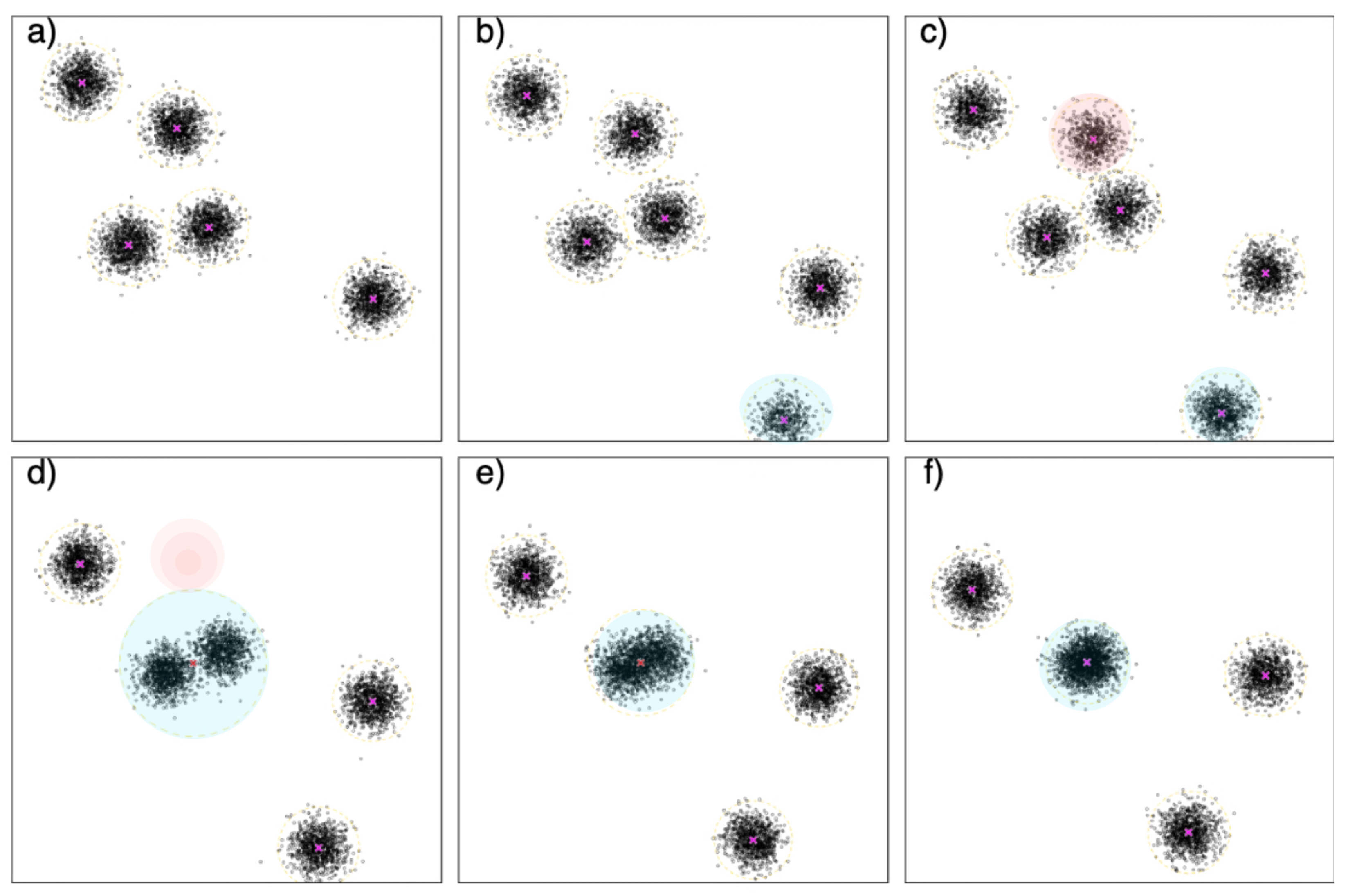
The stream clustering algorithms should handle the dynamic nature of streaming data, in which there is no control over the data arrival order, and the underlying data distribution can change over time. Such changes can be reflected in data clusters [23]. To illustrate such changes in Gaussian data distribution over time, assume that we look at the data stream in six moments represented in Figure 2a–f. Initially, Figure 2a illustrates five data distributions. After this, a new data distribution appears (which can be gradual or abrupt), shown in Figure 2b,c. Moreover, some data distributions can disappear, highlighted in red in Figure 2c,d, or merge with existing ones. Figure 2d,e illustrate two data distributions that are becoming closer over time, and then they merge, forming one dense data distribution, as in Figure 2f.

Initially introduced in [13], this section presents three evolutionary algorithms developed and compared in the present study, designed to cluster scalable batch streams and dynamically estimate the number of clusters. In [12], the algorithms use sequential and parallel approaches to process data objects one-by-one, respecting the data points’ sequence, such as traditional data stream clustering algorithms. However, the analysis of single objects sequentially shows a severe computational bottleneck towards the distributed processing. In advance of the present work, all the compared algorithms used the Discretized-Stream (DS) [11] approach to properly handle the data streams in the MapReduce model, taking full advantage of the distributed computation and scalability of the framework. In the DS model, the t-th micro-batch $B_t$ consists of an unsorted set of data points $B_t=\{x_p,x_{p+1},\dots ,x_{p+q}\}$, where p is the offset of the micro-batch and q is the size of the micro-batch. A micro-batch $B_t$ can be interpreted as one of six scenarios illustrated in Figure 2 from a to f. When the micro-batch arrives, it is distributed through the nodes of the system so that $b_1\cup b_2\cup \dots \cup b_m=B_t$, where m is the size of the distributed system, and $b_j$ represents a subset of $B_t$ stored in a node. Note that MapReduce implementation replicates all the data in a few nodes to ensure reliability and fault tolerance. Moreover, the time window established by the DS model is the union set of the last micro-batches $W=B_t\cup B_{t-1}\cup \dots \cup B_{t-\left|W\right|}$, where $\left|W\right|$ is the window size. Note that the time window is not a computational resource limitation but a forgetting mechanism related to the data evolution [1].

3.1. SESC

Scalable Evolutionary Stream Clustering (SESC) [13] is an evolutionary algorithm able to cluster batch streams by using the largely widespread data summarization [3]. The algorithm has two main steps, the data summarization (abstraction phase), done over distributed data, and the data clustering (clustering phase), performed by applying F-EAC over the summarized data.

The data are summarized as micro-clusters [22], which have four components: n (the number of data points), $ls$ (the linear sum of the data points), $ssq$ (the sum of squared data points), and $ts$ (the timestamp of the most recent data point of the micro-cluster). Given a micro-cluster M formed by a set of data points $M=\{x_1,\dots ,x_n\}$, where n is the number of data points belonging to it, the linear sum of M is given by a vector $ls={\sum }_{i=1}^n{x}_i$ and its sum of square $ssq={\sum }_{i=1}^n{x}_i^2$. The representative of a micro-cluster M is given by its centroid (mean vector from data points of M) $m=\frac{ls}{n}$. Micro-clusters have two relevant capabilities: the incrementality, which allows adding a single point i to a micro-cluster j (by summing up $x_i$ with the components of $M_j$, $x_i+l{s}_j$ and $\left(x_i\right)ˆ2+ss{q}_j$), and the additivity, which allows combining two micro-clusters, simply adding their three first components (n, $ls$, and $ssq$) and taking the maximum $ts$. An outdated $ts$ (related to the time window) means that the micro-cluster is no longer updated.

Figure 3 shows an overview of the algorithm. When the t-th micro-batch is received, the objects are distributed through the nodes by the DS framework. When the accumulated objects (micro-batch) are delivered to SESC, each node works in a parallel and independent way to maintain a set of q micro-clusters. After the initial micro-clusters are obtained by applying k-means in the first portion of data, the received objects (by the node) are inserted into the micro-cluster model according to the CluStream update method [22]: a data point $x_i$ is inserted into a micro-cluster $M_j$ if the Euclidean distance between $x_i$ and the centroid $m_j$, $dist(x_i,m_j)={\parallel x_i-m_j\parallel }_2$, is less than the $m_j$ boundary; otherwise, a new micro-cluster is created considering the $ls=x_i$, $ssq=\left(x_i\right)ˆ2$, and $n=1$. There is a threshold for the number of micro-clusters (q); thus, an extra action is necessary to fix the model when the limit is exceeded. They are removed if there are outdated micro-clusters ($ts$ is outside of the time window). Otherwise, the closest pair is merged into a single micro-cluster.

When all the nodes finish the micro-cluster model update, which is executed in parallel, a set composed of the union of all the micro-clusters (from all the nodes) is used as weighted data points by the centralized F-EAC algorithm in order to estimate the number of clusters and build a (macro-)clustering model. It is expected that the number of micro-clusters is higher than the number of macro-clusters ($q>>k$) and much smaller than the data stream size ($q<<n$). Thus, it is expected that the centralized system can handle the summarized data.

3.2. ISESC

Differently from SESC, the Incremental Scalable Evolutionary Stream Clustering (ISESC) [13] was designed to cluster raw data directly instead of summarizing them into micro-clusters. Storing the data requires more resources such as memory and processing time than micro-clusters but provides more information and higher accuracy. Distributed and scalable frameworks (such as MapReduce) were designed to provide such resources. SF-EAC provides the first macro-clustering model over an initial data portion, using distributed and parallel computation. These macro-clusters use a data structure extended from the micro-cluster concept, providing incrementality and additivity capabilities. Besides the components n, $ls$, $ssq$, and $ts$, the macro-cluster structure also keeps the lowest simplified silhouette index (SS) value ($lss$) among its data points. The SS index considers the compactness and the separation of the data point $x_i$ belonging to a micro-cluster $M_j$, which are represented by two terms, $a_i$ and $b_i$, respectively. Specifically, the $a_i$ term is given by $dist(x_i,m_j)$ and $b_i=dist(x_i,m_c)$, where $m_c$ is the closest neighbor micro-cluster centroid to $m_j$. Then, the SS index is calculated as $SS\left(x_i\right)=1-\frac{a_i}{b_i}$. The average SS index for all data points gives an estimate of full clustering quality, which ranges from 0 to 1 (under k-means assumption). The cluster radius ($rd$) can be calculated according to Equation (1), which results in the standard deviation, and $\alpha$ defines how many standard deviations compose the radius ($\alpha \ge 1$).

$$rd=\alpha \sqrt{\frac{ls}{n}-{\left(\frac{ss}{n}\right)}^T\left(\frac{ss}{n}\right)}$$

(1)

Figure 4 presents an overview of ISESC. After SF-EAC clusters the first micro-batch, the incremental update component of the algorithm updates the model with new data from the following micro-batches. If the component detects a change (concept drift) during the update, the full-clustering component (SF-EAC) is executed to estimate the number of clusters and build a new model.

Inspired by FEAC-Stream [23], the incremental update component searches for evidence of a significant change (e.g., the emergence of a new cluster) and, if there is none, updates the clusters incrementally. For each data point, the component calculates the shortest Euclidean distance between the point and the centroids (d), and its SS value ($ss$) [21] associated with the closest cluster. Evidence of a significant change is a data point for which d is higher than the radius of the closest cluster ($rd$) or has an SS value inferior to the lowest SS value of the points of the associated cluster ($ss<lss$). If any data point of the micro-batch matches this evidence criterion, the full-clustering component is executed; otherwise, the associated cluster is updated, and the incremental update component continues. All distances, SS, and tests of evidence are made in a distributed fashion through map jobs of MapReduce.

The evidence criterion is represented and visualized as two boundaries for each cluster. Figure 5 is a partial representation of a bi-dimensional clustering model, where $C_3$ and $C_4$ are cluster centroids and $p_i:i\in \{1,2,3,4\}$ are data points. The dotted lines represent the clusters’ radius ($rd$) boundaries, and the dashed lines represent the irregular and convex lowest simplified silhouette ($lss$) boundaries given by the SS function. In this illustrative scenario, $p_1$ is within the $lss$ boundary of $C_3$ but not within that of $rd$. The $lss$ boundary can assume such irregular and wide areas that may even encompass new clusters, and then this object will be treated as evidence of a significant change. In turn, $p_2$ is within overlapping $rd$ boundaries but is not within any $lss$ area. Inserting $p_2$ in either $C_3$ or $C_4$ may not be considered correct, as it does not truly merge these two clusters. Thus, $p_2$ will also be treated as evidence of a significant change (cluster merging). Note that $lss$ areas will never overlap since they grow towards the Voronoi diagram, and k-means always consider the minimum distance. The data point $p_3$ is outside both boundaries and will be treated as evidence of a significant change. The last data point, $p_4$, lies within both boundaries of $C_4$ and does not represent evidence of a significant change.

If evidence of change is detected, the model is incrementally updated. A reduce job assigns the data points to their closest clusters, aggregating their summaries and incrementally updating their information. Then, clusters not updated in the most recent time window, i.e., with $ts$ values older than the time window limit, are removed from the model. The remaining updated clusters compose the new model.

Otherwise, if evidence of change is detected, the full-clustering component is executed over the data of the present time window. It consists of running SF-EAC over an initial population of pre-defined solutions built from the current model and derivatives. The current model reflects the known structure along the data stream. Based on this model, two methods are used to derive it: the first aims at increasing iteratively the number of clusters k until a limit $k_{max}$ is reached, selecting prototype candidates among the farthest objects from the existent centroids (inspired by [18]); the second method aims at decreasing k by merging the closest pairs of clusters repeatedly until a $k_{min}$ cluster is reached. The closest pair of clusters is estimated by their boundaries, i.e., the distance between centroids minus the sum of their radii values ($rd$). If necessary, both methods may use other arbitrary stopping criteria (the maximum population size, for example). Besides guided initialization, SF-EAC provides different strategies to diversify the population during the evolutionary search, estimating a new data-adjusted model.

ISESC incrementally updates the model with a low computational cost when no significant change is detected. However, it runs the full-clustering component at any evidence of change, which is the most accurate (but costly) way to learn the current clustering model. Thus, ISESC prioritizes quality and is suitable for data sets with low concept drift, i.e., the clusters do not or rarely change abruptly. Otherwise, the full-clustering component may be triggered repeatedly, requiring computational resources.

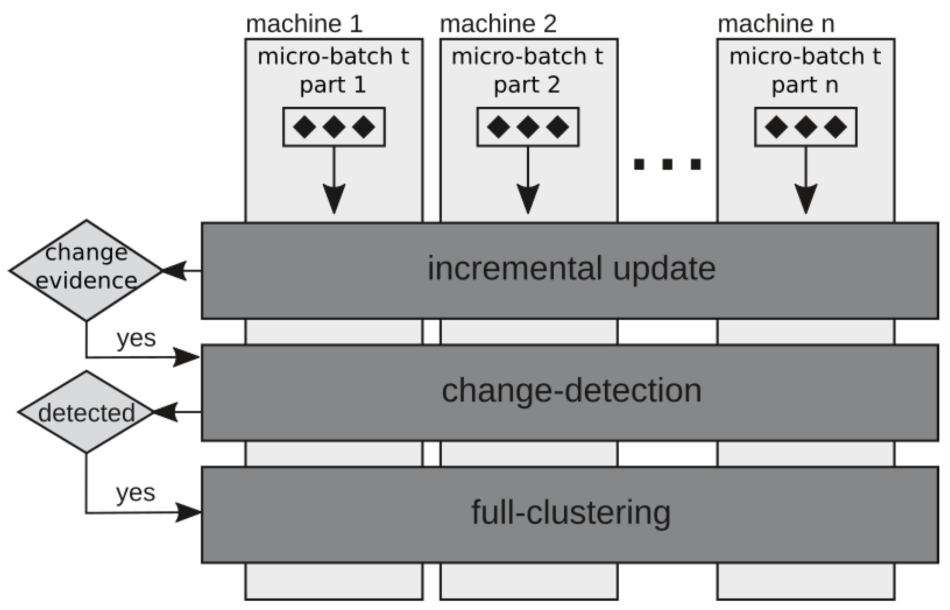
3.3. ISESC-CD

Incremental Scalable Evolutionary Stream Clustering with Change Detection (ISESC-CD) [13] is an extension of ISESC with one additional heuristic component, an attempt to avoid unnecessary executions of full clustering. The change-detection component (CD) resides between the incremental update and full-clustering components, as shown in Figure 6. This component addresses five types of data stream changes detected by the incremental update component: (i) the displacement of an existing cluster in space; (ii) the emergence of a new cluster; (iii) the split of an existing cluster caused by the arrival of objects that leads two or more parts of the cluster in different directions; (iv) the disappearance or expiration of an existing cluster according to its $ts$ and the time window; (v) the merging of two existing clusters, as they incrementally overlap each other. The role of CD is to distinguish the displacement of the clusters (case i) from the others, as cases ii and iii increase the number of clusters k, while cases iv and v decrease it. Applying k-means is enough to deal with cluster displacements, while the full-clustering component is required to estimate models with variations of k.

The model’s change is detected by comparing the current model with two derivations of it. The first derivation results from adding the farthest object from the centroids of the model as a new centroid, increasing k by one. The second results from merging the closest pair of clusters according to its boundaries (the distance between the centroids minus the sum of their radii), decreasing k by one. Both derivations and the current model are fine-tuned by distributed k-means, and then compared among themselves in terms of SS index values. If the current model is the best evaluated, it is preserved. Otherwise, significant evidence of change is detected, and the full-clustering component builds a new model.

Although the full-clustering component is essentially SF-EAC, other clustering algorithms may be considered since the incremental update and change-detection components work regardless of the full-clustering and vice versa. This structure, named Incremental Scalable Stream Clustering with Change-Detection (ISSC-CD), allows the exploration of new batch stream clustering algorithms from non-stream ones.

3.4. Computational Complexity Analysis

For the worst-case scenario, the asymptotic computational complexity of the evolutionary algorithms presented in this work for single micro-batch processing is shown in

Table 1. Asymptotic computational complexity analysis of the evolutionary algorithms.

Algorithm	Worst Case
SESC	$O((n_{mb}\ast d\ast mc)/m)$
ISESC	$O\left(\right(n_w\ast d\ast k_m\ast i\ast g\ast \left|P\right|)/m)$
ISESC-CD	$O\left(\right(n_w\ast d\ast k_m\ast i\ast g\ast \left|P\right|)/m)$

. The size of the micro-batch is given by $n_{mb}$, d is the dimensionality of the data, $mc$ is the number of micro-clusters, m is the number of worker nodes of a distributed system, $n_w$ is the size of the landmark window, $k_m$ is the maximum number of clusters found during the process, i is the maximum iterations of k-means, g is the maximum generations of F-EAC-based algorithms, and $\left|P\right|$ is the population size.

Although the three algorithms have linear complexity in relation to the stream/micro-batch size, for most scenarios, $mc<\frac{n_w}{n_{mb}}\ast k_m\ast i\ast g\ast \left|P\right|$, which gives SESC a lower boundary than ISESC and ISESC-CD.

4. Scalable Distribution-Based Clustering Algorithms

We propose three novel scalable clustering algorithms based on goodness-of-fit tests, i.e., test the data set against a reference distribution. Their goal is to test the hypothesis that specialized approaches to clustering Gaussian-distributed data can improve the accuracy of clustering in the scenario of high-speed data streams.

4.1. SGMS

Scalable G-Means for Stream (SGMS) is based on the scalable version of G-means (SG) [10]. The algorithm has the same incremental update and change-detection components described for the ISESC-CD in Section 2 but adopts the SG procedure in the full-clustering component instead. When its change-detection component triggers, the full-clustering component is executed over the data in the time window (X). It applies SG to estimate the number of clusters and build a new model. Starting from one cluster with all the data, SG consists of iteratively splitting the unstable clusters of the model, i.e., clusters that did not fit the Gaussian distribution. The process is repeated until all clusters fit the Gaussian distribution with a prior-defined confidence level and become stable. Other stopping criteria may be adopted, e.g., a maximum number of splits or iterations. In order to reduce the computational cost, the goodness-of-fit tests are applied over one-dimensional projections of the clusters. G-means is guided by the goodness-of-fit of Gaussian distribution over the clusters, which assumes that the structures of the data sets resemble this distribution. Consequently, such an assumption holds for SG and SGMS.

An overview of SG is presented in Algorithm 1. It starts with two sets: A for unstable clusters and B for stable ones. Thus, the current partition of each iteration is defined by $A\cup B$. The first cluster $c_1$ is built from the mean of X and added to A. The algorithm begins its iterations by assigning each data point with its closest cluster of the current partition using a map job (line 5). Following this, a subset $w_j$ of data points is created for each unstable cluster $a_j$, $\forall j\in A$. A job maps each data point $x_i$ into a pair of <j, $x_i$>, where j is the index of the assigned subset. At line 7, the scalable version of k-means is executed for each subset $w_j$ with $k=2$, as defined in the original G-means [20]. Usually, during the execution of the scalable version of k-means, each data point is mapped with the index of its cluster as a key [24]. However, the clustering of each subset $w_j$ must be done independently, i.e., isolated from the others. Such independence is provided by mapping the data points with keys formed by the index of their clusters and their subset index j. This independence allows the partitioning of all clusters at once by a single pair of maps and reduce jobs by k-means iteration. The result is a set of models $m_j$ obtained for each $w_j$ subset, which is used to create a collection of projection vectors [20] (line 8). In line 9, a map job is used to project each data point within $w_j$ against its projection vector $v_j$. After this, each subset $p_j$ of the projected data points is shuffled through the distributed system to fit a single node and allow the Anderson–Darling (AD) statistical test application. Each $p_j$ is sorted in parallel by the nodes, and the test is applied with the confidence level $\alpha$, yielding a set of statistics $t_j$ (line 10). For each j, if the statistics of $t_j$ accepts the null hypothesis that $p_j$ fits the Gaussian distribution, its original cluster $a_j$ is considered stable and moved to B. Otherwise, the cluster $a_j$ is split, which means adding into A the clusters $m_j$ resulting from $w_j$, and deleting their original cluster $a_j$. The iterations continue until the algorithm reaches a stop criterion (line 4). The algorithm stops if all clusters are stable or a predefined maximum number of iterations is reached in this work.

Algorithm 1: SG overview

4.2. SPGMS

The second algorithm proposed, Scalable PG-Means for Stream (SPGMS), is based on our scalable version of PG-means [19], called SPG-means. We chose PG-means rather than G-means as the former achieved higher-quality results on no incremental batch clustering in [19]. Similar to SGMS, SPGMS has the same incremental update and change-detection components described for the ISESC-CD in Section 2, replacing the full-clustering component with SPG-means.

SPG-means consists of learning one cluster by iteration, beginning from the single-cluster partition. In each iteration, a statistical test is used to verify the goodness-of-fit of the model against the data under several projections and decide whether to create or not a new cluster. If so, the algorithm derives new clusters from the learned ones based on different prototypes: some are randomly selected (to promote diversity); others are chosen among the data points most unfit for the test (to promote intensification). After this, the algorithm refines the selected clusters and adds the best-evaluated to the current clustering model.

A more detailed view of SPG-means is presented in Algorithm 2. A scalable version of the expectation-maximization (EM) algorithm [25] initializes the model M for $k=1$ at line 2. Similar to PG-means, SPG-means executes the Kolmogorov–Smirnov test (KS) [26] under several projection vectors V (built at line 3) in order to reinforce the goodness-of-fit of data against the model. The number of projections r is an input parameter and may be defined as $-2.6198·log\left(ϵ\right)$, being $ϵ$ the desired error rate, as presented in [19]. In line 4, a distributed map job projects the data points of the whole time window (X) over the projection vectors V. The result is $\left|X\right|\ast r$ pairs, where the projection index j is the key, and the projected value is the pair value. Additionally, the centroids of the clusters in the model M are also projected against the same projection vectors V (line 5), but in a centralized way this time, as the number of centroids is small and can be quickly calculated.

Algorithm 2: SPG-means overview

   The sixth line of Algorithm 2 consists of testing the goodness-of-fit of projected data against the projected model. In order to obtain the KS statistics, each $p_j$ for all $j\in V$ must be sorted and ranked. The sort and rank implementations of Apache Spark [25] were used, and its return is a rank index for each object of the data set. The projected data point and rank index are used in a map job to obtain: (i) the cumulative probability of each data point, given the distribution mixture of the projected model $m_j$, and (ii) the distance between the cumulative probabilities of the projected data and model. Then, a reduce job is used to apply the supremum math function in order to obtain the KS statistics. Finally, the result is compared with the critical values to reject or accept the null hypothesis of both data and model belonging to the same distribution mixture.

If the KS test results show that the projected data fit the model for all the projection vectors V, the algorithm returns the model (line 8 of Algorithm 2). Otherwise, it learns the presence of a new cluster and increases k. In line 11, ten data points are selected as prototypes of the new clusters, half selected randomly and the other half through guided selection. This selection is made by using a probability density function to find the five points most unfitted to the distribution mixture because these points have a high probability of representing an unlearned cluster. After this, each selected prototype is inserted into a new model derived from the learned one ($M+c_{k+1}$), refined by the scalable version of EM, and evaluated by likelihood. The best model ($M_l^{\prime }$) from the selected ten replaces M at the next iteration, and k is incremented. If $k_{max}$ is reached, the model M is returned. Otherwise, the process iterates once more, starting at line 3.

4.3. SPKMS

The latest algorithm proposed in this work, Scalable PK-Means for Stream (SPKMS), is a derivation of SPGMS that aims to improve the computational complexity of the scalable EM algorithm, known to be costly [27]. Furthermore, the authors of PG-means [19] suggested other clustering algorithms as an alternative for EM if processing time is relevant. Following such advice, we have chosen k-means due to its influence and low computational complexity. While EM clusters data as a mixture of distributions, k-means partition the data, which may obtain different results.

Presented in Algorithm 3, the SPK-means performs projections over data and model and uses KS statistics to test their goodness-of-fit, similarly to SPG-means (Algorithm 2). If a projection leads KS to reject the null hypothesis that the data and model belong to the same distribution, SPKMS prepares to learn a new cluster. In line 10, the algorithm selects ten new prototypes C: half of them randomly, and the other half are the farthest data points from the current centroids, as done in k-means++ [18]. This selection is made by a map job, which calculates the distance between each data point and its closest centroid, followed by a reduce job, which obtains the farthest data point. In line 11, a set of ten models $M^{\prime }$ are derived from the already learned one (M), each containing one of the selected prototypes C.   

Algorithm 3: SPK-means overview

   In line 12 of Algorithm 3, a scalable version of k-means refines the set of models $M^{\prime }$, using each data reading to update all the models at once. Then, the scalable version of the SS index evaluates the refined models $M^{″}$ in parallel and replaces M with the best-evaluated model. Similar to SPG-means, M is returned if $k_{max}$ is reached; otherwise, the process continues iterating from line 3.

4.4. Computational Complexity Analysis

Our three optimization methods based on the model distribution have two cases: the worst-case scenario, where the full clustering (G-means, PG-means, or Pk-means) must be used and reused to update the model from scratch; and the best-case scenario, which occurs when full clustering is not needed. Both cases are presented in

Table 2. Asymptotic computational complexity analysis of the model-based algorithms.

Algorithm	Worst Case	Best Case
SGMS	$O(n_w\ast k_mˆ2\ast d\ast i)/m)$	$O((n_w\ast k_m\ast d)/m)$
SPGMS	$O(n_w\ast k_mˆ2\ast dˆ3\ast l)$	$O((n_w\ast k_m\ast d)/m)$
SPKMS	$O(n_w\ast k_mˆ2\ast d\ast i)$	$O((n_w\ast k_m\ast d)/m)$

. The size of the micro-batch is given by $n_{mb}$, d is the dimensionality of the data, $mc$ is the number of micro-clusters, m is the number of worker nodes of a distributed system, $n_w$ is the size of the landmark window, $k_m$ is the maximum number of clusters found during the process, i is the maximum iterations of k-means, g is the maximum generations of F-EAC based algorithms, $\left|P\right|$ is the population size, and l is the number of EM iterations.

The main difference in the computational cost of SPGMS and SPKMS resides in the data dimensionality: the former requires a matrix inversion for EM, which implies an $O\left(d^3\right)$ cost; the latter uses a k-means, which is linear considering the data dimensionality d for most common distance measures. Such a characteristic makes SPGMS unfeasible for data sets with high dimensionality, scenarios for which SPKMS is preferable. Both algorithms need a sort step bounded by $O(nlogn)$. However, as $logn<<k\ast d$ holds for most scenarios, other parts of the algorithms asymptotically dominate this step.

5. Experiments

In this section, we experimentally compare the presented algorithms among themselves. The reason for this is that, to the best of our knowledge, there is no other published clustering algorithm in the literature for data streams implemented on top of the MapReduce model (which provides scalability, reliability, resilience, and flexibility) that can estimate the natural number of clusters from a data stream automatically. We analyzed the experimental results qualitatively, through the Adjusted Rand Index (ARI) [28], and in total processing time. The ARI returns the value of 1 when the compared partitions are identical and is adjusted to 0 when comparing random partitions.

5.1. Experimental Setup

All the algorithms were implemented in Scala 2.11, using Apache Spark 2.3 (http://spark.apache.org/, accessed on 20 May 2022) to implement MapReduce and Spark Streaming (http://spark.apache.org/streaming/, accessed on 20 May 2022) as the Discretized-Stream implementation. The experiments were run in a cluster with ten commodity computers providing 60 processing cores ($3.5$ GHz) and 73 GB (35 GB usable by JVM) of RAM. For better estimation of results, each algorithm was repeated twenty times. It is important to note that the scalability inherited from MapReduce allows the replication of the experiments with larger and more sophisticated systems.

We selected seven data sets for our experiments, four built with Gaussian-distributed clusters and three data sets from real applications (

Table 3. Characteristics of artificial and real data sets: the name and type of each data set, their numbers of attributes and instances, and the range of the number of clusters.

Data Set	Type	Attributes	Instances	# of Clusters
100k5-2	Artificial	10	${10}^5$	3…7
1M5-2	Artificial	10	${10}^6$	3…7
1M10-5	Artificial	10	${10}^6$	5…15
10M10-5	Artificial	10	${10}^7$	5…15
KDDCup99 (10%) [30]	Real	34	494,021	2…6
PaperAbstracts [12]	Real	5871	$6.65\times {10}^4$	2…6
YouTube Games [31]	Real	1000	$8.79\times {10}^4$	2…7

). The data stream generator consists of an adaptation of RandomRBFGeneratorEvents [29], which replaces the default uniform randomizer with a Gaussian one. The artificial data sets aim to demonstrate the compared algorithms on different combinations of data size and number of clusters, besides testing the hypothesis presented previously (specialized approaches to clustering Gaussian-distributed data can improve the accuracy of clustering in scenarios of high-speed data streams). On the other hand, the real data sets represent different challenges for the algorithms since they do not strictly follow a distribution mixture. The well-known KDDCup99 (10% version) data set [30] (KC99) is a set of network connections for intrusion analysis, evaluated over its five-class version (Normal, DOS, PROBE, R2L, and U2R). The YouTube Games data set (YTG) [31], text_game_lda_1000 version, is a set of pre-processed textual features (title, tags, and descriptions) associated with a set of videos about 30 games (the noise class 31 was removed). The PaperAbstracts data set [12] (PPA) is a set of pre-processed scientific paper abstracts of seven different knowledge areas.

Since the real data sets do not have a natural sequence, we allocated the data objects in the stream based on their similarity. Such allocation was made to favor the gradual evolution of the data and provide cluster appearance and disappearance events over time. Therefore, all the data streams were divided into 100 micro-batches.

Considering the PPA and YTG data sets, the cosine dissimilarity was adopted for k-means based algorithms. Unfortunately, SPGMS could not process these data sets due to their high dimensionality, which causes the distributed version of EM (Gaussian Mixture algorithm) to perform poorly [25,32]. Therefore, dimensionality reduction is advised in these cases.

According to studies performed in [33], five iterations of k-means is enough to fine tune most data partitions. Thus, the compared algorithms adopt a limit of five iterations for k-means runs. A study presented in [34] showed a trade-off between the population size and the maximum number of generations of F-EAC. Based on this study, F-EAC-based algorithms evolve a population of 10 individuals for five generations here. SPGMS and SPKMS used $\alpha =0.01$ and 12 projections, and SPGS also used $\alpha =0.01$. The number of micro-clusters of the incremental-update component of SESC was systematically chosen: we executed five repetitions for each data set with $\left|D\right|\times k_{max}\times \beta$ micro-clusters, where $\left|D\right|$ represents the size of the distributed system (10 for this work) and $\beta \in \{1,2,3,4,5\}$. The executions showed that increasing $\beta$ also increases the processing time but does not improve the quality of the model; thus, $\beta =1$ was adopted. For all the algorithms, except SGMS, $k_{min}=2$ and $k_{max}=2\times c_{max}$, where $c_{max}$ is the upper bound of the class number range for a data set. SGMS was limited to 6 iterations, which allowed the production of up to $2^6$ clusters.

The Shapiro–Wilk test [35] rejected the normality hypothesis over most of the experimental results regarding ARI values and computing time, which is not recommended for parametric statistical tests. Thus, the non-parametric test of Friedman was adopted with 95% significance over all the results presented here, followed by Fisher’s least significant difference (LSD) for multi-comparisons [36]. The results from the tests indicate whether the algorithms have differences in quality/time, with 95% significance, being significantly better or worse than another.

5.2. Qualitative Analysis of Quality

A qualitative quality analysis, measured by ARI, among the six algorithms and over the most representative data set results, is presented in the charts of Figure 7. The vertical axis represents the average ARI score values, and the horizontal axis measures the micro-batch position in the stream from 1 to 100. For each algorithm, the markers indicate the average of ARI, and the vertical grey bars are their standard deviations. Note that concept drift and concept evolution in the data streams cause variations in quality, reflected by the ARI scores. The charts show discrepancies in the algorithms’ behaviors for different data sets. One of the most notable discrepancies resulted from SGMS in the real data sets (the right arrows in Figure 7c–e). SGMS overestimated the number of clusters up to six times more that of other algorithms for such data sets, which caused a decrease in its ARI values. Similar to [19], the split policy inherited from G-means overestimated the number of clusters here. SPGMS had better quality than SGMS in the KDD data set because the goodness-of-fit test inherited from PG-means was designed to deal with the G-means overestimation of k. However, SPGMS was shown to be computationally prohibitive for high-dimensional data sets. Fortunately, SPKMS had good performance and we found that its goodness-of-fit test, inherited from PG-means, dealt with the k overestimation, even in scenarios with scalable batch streams. Over artificial Gaussian data sets, the SGMS algorithm performed as well as the other algorithms.

It is notable that SESC presented a lower-quality result during the micro-batches from 71 to 80 of 100k5-2 (Figure 7a) compared to the other algorithms. In this scenario, the granularity and density of the micro-clusters were not sufficient to detect two close clusters with the SS index, which caused SESC to underestimate the number of clusters and, consequently, impacted the ARI.

For most scenarios, ISESC and ISESC-CD have similar quality, which is expected since their only difference is the change-detection component. However, there are some punctual differences, as presented in the periods between the micro-batches 48 and 52, 67, and 74 of the YTG data set. In such periods, the ISESC can promptly detect changes in the data stream, while the ISESC-CD needs more time to discover (and react) to these changes. A different scenario occurred for the PPA data set, where the SS index that guides the F-EAC did not behave similarly to the ARI, as described in [12]. Such behavior caused significant ARI differences between ISESC and ISESC-CD, mainly between micro-batches 5 and 20 and between micro-batches 56 and 75. In both intervals, ISESC replaced the model with a better-evaluated one (according to the SS index), while ISESC-CD incrementally updated its current model. As the SS and ARI indexes do not behave similarly to PPA, the increase in the SS value in ISESC caused a decrease in its ARI values. Figure 8 shows how ISESC was slightly better in terms of SS, when compared to ISESC-CD in the same intervals.

5.3. Quantitative Analysis of Quality

The quantitative analysis presented here compares the scores of the algorithms among themselves. In terms of ARI, the algorithm’s score is the number of micro-batches (out of 100) for which the algorithm has the best or statistically equivalent result. For each data set, these results are tested over the repetitions of the algorithms. High scores indicate that the algorithm obtained better-quality results more often. For example, the algorithm SGMS achieved the best-quality result (or statistically equivalent) for 88 out of 100 micro-batches over the data set 100k5-2.

Table 4. ARI rank scores. The table shows in how many micro-batches the algorithm was the best, in terms of ARI, or statistically equivalent to the best. The bold cells highlight the best algorithm for each data set.

Data Set	SESC	ISESC	ISESC-CD	SGMS	SPGMS	SPKMS
100k5-2	42	83	83	88	37	86
1M5-2	40	65	65	68	29	78
1M10-5	25	51	52	49	47	73
10M10-5	30	64	65	22	19	65
KC99	34	74	78	1	11	62
YTG	74	53	44	0	0	62
PPA	70	38	71	0	0	46
Total 1	171	337	343	228	143	364
Total 2	315	428	458	228	143	472

shows the score of each algorithm over each data set. The bold cells highlight the highest sum of points for each data set. For fairness, Total 1 sums the scores for the data sets with moderate dimensionality, which could be processed by SPGMS (100k5-2, 1M5-2, 1M10-5, 10M10-5, KC99). Total 2 summarizes the score for all the data sets.

ISESC and ISESC-CD produced similar-quality results, mainly on artificial data sets, as shown in Table 4. Moreover, ISESC-CD was even better than ISESC in some 1M10-5, 10M10-5, KC99, and PPA micro-batches. This result evidences that the change-detection component of ISESC-CD did not affect the algorithm’s quality in most scenarios. A similar result is presented in [13].

SESC performed worse than ISESC and ISESC-CD for most data sets, except for PPA and YTG. It is interesting to note that SESC performed better than other algorithms in specific situations, such as in the interval between micro-batch 43 and 76 of YTG or 21 and 33 of PPA (as shown in Figure 7d and Figure 7e, respectively). Reflecting on the ARI values, such intervals contain overlapping clusters, and SESC could detect and learn them better. Summarizing data on micro-clusters smooths the overlapping of clusters for the SS evaluation compared to raw data. Sometimes, this smoothness improved the SS evaluation, resulting in higher ARI values. Such an effect rarely happens for algorithms that analyze raw data. It is important to note that the systematic definition of the number of micro-clusters, described at the beginning of Section 5, improved the quality results for YTG and PPA concerning [13].

SGMS produced high-quality results for 1M5-2 and 1M10-5, the best algorithm for 100k5-2. Such results reside in the well-behaved Gaussian clusters of these data sets, the best scenario for SGMS. However, low-quality results were obtained for 10M10-5, mainly due to the increased number of clusters overlapping in the last 30 micro-batches. On real data sets, SGMS was the worst algorithm (also shown in Figure 7). It did not even obtain a score on the PPA and YTG data sets. This occurred because SGMS inherited from G-means the drawback of overestimating k in non-Gaussian-distributed clusters.

The quality of the SPGMS results is worse than the SGMS ones, although the opposite was presented in [19] for their centralized counterparts when evaluating other validation indices. SPGMS is not guided by the SS index, unlike other algorithms, using likelihood instead. SPGMS achieved the worst result for 10M10-5. This result is derived from the fact that close to 96% of the full-clustering runs of SPGMS (using EM) over the data set overestimated the number of clusters, stopping at the defined upper bound. A different behavior was presented by SPKMS, which also uses projections and tests the goodness-of-fit. Such results indicate that models that were refined by EM and evaluated by likelihood performed worse than those that were refined by k-means and evaluated by SS in our experiments.

SPKMS produced quality results for both artificial and real data sets. Moreover, it had a better score than SPGMS for all data sets and was able to cluster high-dimensional data sets (PPA and YTG). Moreover, it was the best algorithm for the 1M5-2, 1M10-5, and 10M10-5 data sets (Table 4). The quality of SPKMS results from the combination of four characteristics: (i) a systematic method to decide whether to increase k, guided by goodness-of-fit tests and inherited from PG-means; (ii) the seeding of the new prototypes based on k-means++; (iii) the refinement of models by k-means and, (iv) the selection of the best partition by the SS index.

Based on the ARI scores in Table 4, SPGMS presented the worst results for most data sets that it was able to process, and SPKMS was the best algorithm in most scenarios, followed by ISESC-CD, ISESC, SESC, and SGMS. Furthermore, SPKMS was the best-evaluated considering normally distributed data sets, and SGMS was shown to be more accurate than SESC. Note that the clusters of the real data sets do not need to fit the Gaussian distributions, i.e., the goodness-of-fit tests are not expected to fit all data sets. However, SPKMS was among the best results for most of these data sets.

5.4. Processing Time Analysis

Table 5. Average execution time comparison in minutes [$\mu$ ($\sigma$)]. The bold cells highlight the best algorithm, or statistically equivalent, for each data set.

	SESC	ISESC	ISESC-CD	SGMS	SPGMS	SPKMS
100k5-2	0.78 (0.02)	26.26 (3.04)	5.97 (0.63)	8.76 (0.45)	60.74 (17.23)	33.14 (7.46)
1M5-2	1.03 (0.01)	40.69 (6.97)	12.11 (1.51)	25.59 (1.22)	162.97 (11.75)	151.79 (10.49)
1M10-5	2.75 (0.44)	89.73 (12.52)	20.89 (2.38)	35.70 (3.04)	284.68 (32.12)	316.05 (27.77)
10M10-5	18.38 (3.75)	587.57 (50.84)	83.07 (7.40)	76.27 (9.74)	4273.37 (362.64)	1685.29 (196.06)
KC99	1.18 (0.03)	50.87 (5.89)	16.45 (2.24)	59.52 (4.71)	283.44 (19.16)	106.56 (10.36)
YTG	20.66 (0.72)	263.09 (42.80)	85.33 (13.28)	178.34 (18.25)		187.29 (26.10)
PPA	67.10 (4.32)	666.61 (36.20)	99.90 (10.05)	171.29 (26.03)		279.87 (47.29)
Total 1	23.46 (4.29)	762.10 (75.70)	134.74 (8.55)	195.26 (6.03)	4958.73 (320.05)	2216.43 (97.10)
Total 2	111.46 (6.08)	1660.93 (102.93)	317.36 (19.99)	537.41 (27.74)		2670.20 (123.19)

presents the processing time comparison (in minutes) among all algorithms. For simplicity, the total execution time of the compared algorithms was considered instead of the time for processing individual micro-batches. Total 1 sums the running time for the data sets processed by SPGMS (100k5-2, 1M5-2, 1M10-5, 10M10-5, and KC99), and Total 2 does the same for all data sets. Every cell represents the average and standard deviation of 20 repetitions, including the totals. The values in bold highlight the fastest algorithm and the ones with no significant difference from the fastest for each data set, according to the Friedman test with 95% confidence. SESC was the fastest for all the data sets. ISESC-CD was faster than ISESC (5.2 times on average, according to Total 2), due to its change-detection component being designed to avoid unnecessary full-clustering processing. This component was able to avoid full-clustering processing 82% of the time. ISESC-CD was also statistically equivalent to the fastest algorithm over most data sets and the totals. However, unlike SESC, it obtained high-quality results (Table 4) for most of the data sets. Because of the expectation-maximization algorithm, SPGMS was the slowest algorithm for most of the data sets, unable to process them all. Designed to overcome this, SPKMS was 2.2 times faster than SPGMS, considering the Total 1 of Table 5. Due to its simplicity, SGMS was the fastest projection-based algorithm, but not so fast as the evolutionary FEAC-based algorithms. SGMS requires many shuffles through the distributed system (as SPGMS and SPKMS). In short, the fastest algorithm was SESC, followed by ISESC-CD, SGMS, ISESC, SPKMS, and SPGMS.

6. Conclusions

In this work, six algorithms designed to cluster scalable stream batches and estimate the number of clusters were experimentally compared. SESC was the fastest algorithm due to its summarizing power, while SPKMS achieved high-quality results for most data sets due to its goodness-of-fit tests over projections, a heuristic for seeding prototypes, and partition refinement by k-means. Moreover, ISESC-CD and ISESC stand out for their quality results, while ISESC-CD achieved competitive processing time. Considering the algorithms based on goodness-of-fit tests, SGMS was the fastest, obtaining quality results for the normally distributed data sets. Additionally, the evolutionary algorithms obtained the best results, in terms of quality, for real data sets. Such results show that our proposed algorithms can complement each other for various application scenarios.

The experiments support our hypothesis that the specialist approach for clustering data sets with normal distribution could improve the accuracy in scenarios of scalable batch streams, as the most accurate results for the normal distribution data sets were reached by SGMS and SPKMS.

As a general guide, a suitable algorithm may be selected according to the distribution of the data set and the available computational resources. The goodness-of-fit-based algorithms (SGMS or SPKMS) should be preferred if normality is expected in the data set. SGMS is faster and can handle scenarios where the available computational resources render the SPKMS unfeasible. However, the latter obtained the results with the best quality. If the clusters are not expected to fit a normal distribution or their distribution is unknown, the evolutionary algorithms, SESC or ISESC-CD, are preferred due to their average quality. SESC is fast and recommended for scenarios with limited computational resources, while ISESC-CD has the best quality, requiring more computational resources. According to the experiments, ISESC and SPGMS did not stand out during the experiments. Although ISESC reached quality results close to ISESC-CD, the former is considerably slower. SPGMS showed that adapting PG-means for distributed and parallel batch streams is burdensome and sometimes unfeasible, as the expectation-maximization step needs to access the data multiple times. However, it inspired SPKMS, the adaptation of SPGMS that uses k-means evaluated by silhouette, which is faster and achieves the best-quality results, one of the main findings of this paper.

Concerning arbitrary-shaped clusters, we intend to investigate how to scale density-based clustering algorithms for this task in future work.

References

1. Gama, J. Knowledge Discovery from Data Streams, 1st ed.; CRC Press: Boca Raton, FL, USA, 2010. [Google Scholar]
2. Gomes, H.M.; Read, J.; Bifet, A.; Barddal, J.P.; Gama, J. Machine learning for streaming data: State of the art, challenges, and opportunities. ACM SIGKDD Explor. Newsl. 2019, 21, 6–22. [Google Scholar] [CrossRef]
3. Silva, J.A.; Faria, E.R.; Barros, R.C.; Hruschka, E.R.; Carvalho, A.C.; Gama, J. Data stream clustering. ACM Comput. Surv. 2013, 46, 1–31. [Google Scholar] [CrossRef]
4. Moulton, R.H.; Viktor, H.L.; Japkowicz, N.; Gama, J. Clustering in the Presence of Concept Drift. In Proceedings of the Machine Learning and Knowledge Discovery in Databases; Berlingerio, M., Bonchi, F., Gärtner, T., Hurley, N., Ifrim, G., Eds.; Springer International Publishing: Cham, Switzerland, 2019; pp. 339–355. [Google Scholar]
5. Naldi, M.C.; Fontana, A.; Campello, R.J.G.B. Comparison Among Methods for k Estimation in k-means. In Proceedings of the Ninth International Conference on Intelligent Systems Design and Applications, Pisa, Italy, 30 November–2 December 2009; pp. 1006–1013. [Google Scholar]
6. Dinh, D.T.; Fujinami, T.; Huynh, V.N. Estimating the Optimal Number of Clusters in Categorical Data Clustering by Silhouette Coefficient. In Proceedings of the Knowledge and Systems Sciences; Chen, J., Huynh, V.N., Nguyen, G.N., Tang, X., Eds.; Springer: Singapore, 2019; pp. 1–17. [Google Scholar]
7. Morales, G.D.F.; Bifet, A. SAMOA: Scalable Advanced Massive Online Analysis. J. Mach. Learn. Res. 2015, 16, 149–153. [Google Scholar]
8. Bifet, A.; Maniu, S.; Qian, J.; Tian, G.; He, C.; Fan, W. StreamDM: Advanced Data Mining in Spark Streaming. In Proceedings of the IEEE International Conference on Data Mining Workshop, Atlantic City, NJ, USA, 14–17 November 2015. [Google Scholar] [CrossRef] [Green Version]
9. Dean, J.; Ghemawat, S. MapReduce: Simplified data processing on large clusters. Commun. ACM 2008, 51, 107–113. [Google Scholar] [CrossRef]
10. Oliveira, G.V.; Coutinho, F.P.; Campello, R.J.; Naldi, M.C. Improving k-means through distributed scalable metaheuristics. Neurocomputing 2017, 246, 45–57. [Google Scholar] [CrossRef]
11. Zaharia, M.; Das, T.; Li, H.; Shenker, S.; Stoica, I. Discretized Streams: An Efficient and Fault-Tolerant Model for Stream Processing on Large Clusters. In Proceedings of the HotCloud’12 Proceedings of the 4th USENIX conference on Hot Topics in Cloud Computing, Boston, MA, USA, 12–13 June 2012. [Google Scholar]
12. Cândido, P.; Naldi, M.C.; Silva, J.A.; Faria, E.R. Scalable Data Stream Clustering with k Estimation. In Proceedings of the 2017 Brazilian Conference on Intelligent Systems (BRACIS), Uberlandia, Brazil, 2–5 October 2017; pp. 336–341. [Google Scholar] [CrossRef]
13. Candido, P.L.; Silva, J.A.; Faria, E.R.; Naldi, M.C. Scalable Batch Stream Clustering with k Estimation. In Proceedings of the 2018 IEEE Congress on Evolutionary Computation (CEC), Brisbane, Australia, 10–15 June 2018; pp. 1–8. [Google Scholar] [CrossRef]
14. Khader, M.; Al-Naymat, G. Density-Based Algorithms for Big Data Clustering Using MapReduce Framework: A Comprehensive Study. ACM Comput. Surv. 2020, 53, 1–38. [Google Scholar] [CrossRef]
15. MacQueen, J. Some methods for classification and analysis of multivariate observations. In Proceedings of the Berkeley Symposium on Mathematical Statistics and Probability, Berkeley, CA, USA, 18–21 July 1965 and 27 December 1965–7 January 1996. [Google Scholar]
16. Wu, X.; Kumar, V. The Top Ten Algorithms in Data Mining; CRC Press: Boca Raton, FL, USA, 2009. [Google Scholar]
17. Alves, V.; Campello, R.J.G.B.; Hruschka, E.R. Towards a Fast Evolutionary Algorithm for Clustering. In Proceedings of the IEEE Congress on Evolutionary Computation, Vancouver, BC, Canada, 16–21 July 2006; pp. 1776–1783. [Google Scholar]
18. Arthur, D.; Vassilvitskii, S. K-Means++: The Advantages of Careful Seeding. In Proceedings of the Eighteenth Annual ACM-SIAM Symposium on Discrete Algorithms, New Orleans, LA, USA, 7–9 January 2007; Volume 8, pp. 1025–1027. [Google Scholar] [CrossRef]
19. Feng, Y.; Hamerly, G. PG-means: Learning the number of clusters in data. In Proceedings of the Advances in Neural Information Processing Systems 19; MIT Press: Cambridge, MA, USA, 2007. [Google Scholar] [CrossRef] [Green Version]
20. Hamerly, G.; Elkan, C. Learning the k in k-means. In Neural Information Processing Systems; MIT Press: Cambridge, MA, USA, 2003. [Google Scholar]
21. Hruschka, E.R.; de Castro, L.N.; Campello, R.J.G.B. Evolutionary algorithms for clustering gene-expression data. In Proceedings of the Fourth IEEE International Conference on Data Mining, Brighton, UK, 1–4 November 2004; pp. 403–406. [Google Scholar]
22. Aggarwal, C.C.; Han, J.; Wang, J.; Yu, P.S. Aggarwal, C.C.; Han, J.; Wang, J.; Yu, P.S. A framework for clustering evolving data streams. In Proceedings 2003 VLDB Conference; Wang, J.; Morgan Kaufmann: Burlington, MA, USA, 2003; Volume 29, pp. 81–92. [Google Scholar]
23. Silva, J.A.; Hruschka, E.R.; Gama, J. An evolutionary algorithm for clustering data streams with a variable number of clusters. Expert Syst. Appl. 2017, 67, 228–238. [Google Scholar] [CrossRef]
24. Meng, X.; Bradley, J.; Yavuz, B.; Sparks, E.; Venkataraman, S.; Liu, D.; Freeman, J.; Tsai, D.B.; Amde, M.; Owen, S.; et al. MLlib: Machine Learning in Apache Spark. J. Mach. Learn. Res. 2016, 17, 1235–1241. [Google Scholar]
25. Zaharia, M.; Xin, R.S.; Wendell, P.; Das, T.; Armbrust, M.; Dave, A.; Meng, X.; Rosen, J.; Venkataraman, S.; Franklin, M.J.; et al. Apache Spark: A Unified Engine for Big Data Processing. Commun. ACM 2016, 59, 56–65. [Google Scholar] [CrossRef]
26. Massey, F.J., Jr. The Kolmogorov-Smirnov Test for Goodness of Fit. J. Am. Stat. Assoc. 1951, 46, 68–78. [Google Scholar] [CrossRef]
27. Bishop, C.M. Pattern Recognition and Machine Learning (Information Science and Statistics); Springer: Berlin/Heidelberg, Germany, 2006. [Google Scholar]
28. Hubert, L.; Arabie, P. Comparing partitions. J. Classif. 1985, 2, 193–218. [Google Scholar] [CrossRef]
29. Bifet, A.; Holmes, G.; Kirkby, R.; Pfahringer, B. MOA Massive Online Analysis. J. Mach. Learn. Res. 2010, 11, 1601–1604. [Google Scholar]
30. Lichman, M. UCI Machine Learning Repository; University of California: Los Angeles, CA, USA, 2013. [Google Scholar]
31. Madani, O.; Georg, M.; Ross, D.A. On Using Nearly-Independent Feature Families for High Precision and Confidence. Mach. Learn. 2013, 92, 457–477. [Google Scholar] [CrossRef] [Green Version]
32. Damji, J.; Wenig, B.; Das, T.; Lee, D. Learning Spark-Lightning-Fast Big Data Analysis; O’Reilly Media: Newton, MA, USA, 2015. [Google Scholar]
33. Anderberg, M. Cluster Analysis for Applications; Academic Press: Cambridge, MA, USA, 1973. [Google Scholar]
34. Naldi, M.C.; Campello, R.J.G.B.; Hruschka, E.R.; Carvalho, A. Efficiency issues of evolutionary k-means. Appl. Soft Comput. 2011, 11, 1938–1952. [Google Scholar] [CrossRef]
35. Shapiro, S.S.; Wilk, M.B. An Analysis of Variance Test for Normality (Complete Samples). Biometrika 1965, 52, 591–611. [Google Scholar] [CrossRef]
36. Conover, W. Practical Nonparametric Statistics; Wiley: Hoboken, NJ, USA, 1999. [Google Scholar]
Figure 1. Relationship between the main data clustering sub-fields: estimation of the number of clusters k (a), data stream (b), and MapReduce (c).
Applsci 12 06464 g001
Figure 2. Illustration of changes in data distribution over time. The blue and red spheres around data highlight such changes, where a new data distribution is emerging in (ac) (highlighted in blue), a data distribution disappears in (c,d) (highlighted in red), and two data distributions are merging over time in (df) (highlighted in blue).
Applsci 12 06464 g002
Figure 3. SESC overview [13].
Applsci 12 06464 g003
Figure 4. ISESC overview, adapted from [13].
Applsci 12 06464 g004
Figure 5. Representation of boundaries used to detect significant change for evidence criterion.
Applsci 12 06464 g005
Figure 6. ISESC-CD overview, adapted from [13].
Applsci 12 06464 g006
Figure 7. ARI comparison among the presented algorithms over the five most relevant data set results. The markers represent the ARI score of each algorithm over each data set. The vertical grey bars represent the standard deviation.
Applsci 12 06464 g007
Figure 8. SS comparison—PPA data set. The vertical axis represents the SS score and the horizontal axis represents the micro-batch position.
Applsci 12 06464 g008