1. Introduction
Object segmentation separates the foreground objects in an image from the background image. Subsequently, object labeling is performed to record the label number, position, and region of each foreground object. Relevant labeling information can be used for subsequent object recognition and tracking. Currently, object segmentation and recognition techniques have been applied to various systems, such as robot vision [
1,
2], autonomous driving [
3,
4], intelligent monitoring [
5,
6], and unmanned vehicles [
7,
8].
Object segmentation can be divided into two categories, dynamic and static image segmentation. In terms of dynamic image segmentation, objects are segmented using the image continuity characteristic of consecutive images. Rychtáriková et al. [
9] proposed information-entropic variables, Point Divergence Gain, Point Divergence Gain Entropy, and Point Divergence Gain Entropy Density, to characterize the dynamic changes in image series. The information-entropic variables can be used to detect and segment moving objects. Wixson [
10] used the motion changes of consecutive and adjacent images to segment foreground objects. The background subtraction algorithm [
11] can accomplish object segmentation by comparing the difference between the background image and the input image. Chiu et al. [
12] used the background subtraction algorithm based on the probability change of pixels in consecutive images to segment foreground objects. In contrast to dynamic image segmentation for consecutive images, static image segmentation involves analyzing the characteristics of the image itself to achieve object segmentation. Static image segmentation typically uses the gray level, color, or edge information of a single image to complete object segmentation. Dirami et al. [
13] used the gray-level histogram of the image to conduct multilevel thresholding analysis and multilevel thresholds to segment objects of different gray levels. Color segmentation [
14,
15,
16] is a process in which pixels of different colors are divided into different categories and objects by color clustering. Because colors are relatively sensitive to changes in light, images are often converted from RGB to other color spaces, such as HSI, CIELAB, and CMYK, to obtain better results. Contour features [
17,
18] use the shape and surface texture as a basis for object segmentation. Object characteristics change drastically near edges and are not easily affected by changes in color or light. Compared with the color segmentation and background subtraction algorithm, contour features are more stable and less restrictive. Therefore, contour features are the information commonly used in most object segmentation studies. Owing to a lack of information regarding consecutive images, static image segmentation is much more difficult than dynamic image segmentation in terms of object segmentation.
Both dynamic and static object segmentation techniques involve the segmentation of overlapping objects in two-dimensional (2D) images. Although dynamic images can use the object movement information to segment the objects moving in different directions, they cannot segment the overlapping objects moving in the same direction. Existing studies have used three-dimensional (3D) information to segment overlapping objects in pair images. Object segmentation techniques based on 3D information can also fall into two types: dynamic and static. For dynamic 3D image segmentation, Xie et al. [
19] extracted keyframes at fixed intervals in consecutive images of RGB-D video and used image and depth information for each keyframe to complete the object segmentation. Although the method can effectively segment complex overlapping objects, it relies on object recognition to segment-specific objects. Considering that the change in motion of moving objects in consecutive images is larger than that of the background image, Liu et al. [
20] combined long-term motion and stereo information and used stereoscopic foreground trajectories to segment the moving objects. Sun et al. [
21] used the gray-level difference at fixed intervals in consecutive images to extract the edges of moving objects, calculated the depth information of the edge points of moving objects, clustered the depth information, and segmented different objects. Although the object segmentation techniques proposed by Liu et al. [
20] and Sun et al. [
21] do not rely on object recognition, they rely on the motion or gray-level difference of objects in consecutive images.
Frigui and Krishnapuram [
22] proposed a 3D fuzzy clustering method to perform clustering analysis for different planes and curved surfaces using the 3D information of images. This method can be applied to segment overlapping objects from static images without complex backgrounds. However, the clustering method requires setting the initial number of categories and repeating the iterative computational analysis. Therefore, this method is prone to classification errors and consumes a lot of computation time. Gotardo et al. [
23] proposed an improved robust estimator and genetic algorithm that uses depth gradient images to analyze different surface regions and uses the surface models of 3D planes and curved surfaces to detect and extract all planes and curved surfaces from 3D images sequentially and iteratively. Husain et al. [
24] used adaptive surface models to segment 3D point clouds into a preset number of geometric surfaces, which were used as the initial setting for image segmentation. Then, they merged similar adjacent surfaces together, recalculated the relevant parameters, and repeated the process until the termination condition was met. This type of method that fits the object surface with 3D surface models to segment different objects also consumes a lot of computation time and is unsuitable for the complex environment.
After object segmentation, the position and label of each object must be analyzed and recorded for subsequent recognition or analysis. The most widely used object labeling method is the connected component labeling algorithm proposed by Rosenfeld and Pfaltz [
25]. First, this method converts all pixels of the objects that are segmented from the 2D image into a binary image, merges adjacent pixels into the same object in sequence, and assigns label numbers to distinguish different objects, thereby achieving the purpose of labeling the position and region of the objects. However, this method requires large amounts of memory to record labels. Haralick [
26] used a multi-scan to reduce the amount of memory used in the labeling process as well as a forward and backward mask to scan the binary image alternately. Although no additional memory was required to record labels, more execution time was required. Many researchers have subsequently proposed improved methods [
27], such as the four-scan, two-scan, one-scan, contour-tracing labeling, and hybrid object labeling algorithms. Although these methods can reduce memory usage or speed up the operation, they can only connect objects in 2D images without integrating the distance information for the overlapping objects.
In summary, the use of 3D information can indeed effectively segment the overlapping objects in images. Compared with dynamic object segmentation, static object segmentation does not require much time to analyze consecutive images. Therefore, this paper proposes a 3D object segmentation and labeling algorithm for static images to segment and label objects simultaneously, to realize object segmentation and labeling in unknown environments. The remainder of this paper is organized as follows.
Section 2 introduces the 3D object segmentation algorithm.
Section 3 presents the relevant experimental results. The applications and contributions of the proposed algorithm are summarized in
Section 4.
2. Three-Dimensional Object Segmentation and Labeling Algorithm
The 3D object segmentation and labeling algorithm proposed in this paper can be divided into four processing steps, namely, the texture construction edge detection algorithm (TCEDA) [
28], distance connected component algorithm, object extension and merge algorithm, and object segmentation. First, TCEDA is used to detect large amounts of edge contours in the images. Second, the distance connected component algorithm detects the distance of each edge pixel and uses the distance information to determine whether the pixels belong to the same line segment and records their label numbers, number of valid points, and coordinates. The above two processing steps may cause line segment fragmentation for two reasons. First, the change in images is not evident; therefore, the edge detection is not complete. Second, owing to the matching error generated during image matching, parts of a line segment are incorrectly detected as having different distances. The third processing step uses the line segment extension and merge algorithm to extend and construct the disconnected line segments. The line segments that satisfy the extension connection conditions are merged into the same line segment. Therefore, the third processing step can solve the fragmentation problems of object contours caused by edge detection and image matching methods. Finally, morphology and run-length smoothing algorithm are used to merge the line segments into different segmented objects, and the 3D information is estimated for each segmented object. Each processing step of the proposed algorithm will be subsequently described in detail in each subsection.
2.1. TCEDA
In this paper, TCEDA [
28] is used to detect edge information in images. The candidate edge points are detected by determining whether adjacent pixels with gradient changes have reasonable texture changes. Then, the edge texture extension method is used to delete relatively short line segments, thereby retaining effective contour edge points. TCEDA can avoid inappropriate threshold setting and retain large amounts of edge information as the object in the next processing step.
TCEDA mainly involves three steps: image preprocessing, optimal edge thinning process, and edge texture construction processing. In image preprocessing, the input color image is converted into a gray-level image. Then, the 2D Gaussian function filter is used for smoothing to reduce the interference caused by noise on the image edge. Subsequently, the Sobel filter mask is used to calculate the gradient value of each pixel in the image. Finally, the gradient amplitude and angle of each pixel are calculated.
In the optimal edge thinning process, the gradient amplitude and angle of each pixel are analyzed using the non-maximum suppression method to obtain the initial result of edge thinning. Subsequently, the redundant pixels processed by the non-maximum suppression method are removed using the thinning texture template process to obtain the optimal result of edge thinning. The non-maximum suppression method classifies the calculated gradient angles based on their similarity and compares the gradient amplitudes of adjacent pixels on both sides of the gradient direction of the processed pixel (center pixel). When the gradient amplitudes of the two adjacent points are both smaller than that of the center pixel, the center pixel and two adjacent points are labeled as candidate edge points; otherwise, they are not labeled. Subsequently, the thinning texture template is used to compare the texture of a 3 × 3-pixel block of the candidate edge point in the raster-scan order. When the block texture conforms to the defined thinning texture template, the redundant pixel in the center of the block is deleted. The optimal edge thinning result can be obtained after all candidate edge points are processed.
Because the optimal edge thinning process retains many short line segments and isolated points, the edge texture construction processing is used to delete these noises (short line segments and isolated points) and retain long line segments with extensible texture changes. The edge texture construction processing extends and constructs line segments by expanding the edge texture template established between adjacent blocks. In this process, the extended length of the edge line segment containing more than six edge points is retained to obtain the edge contour image.
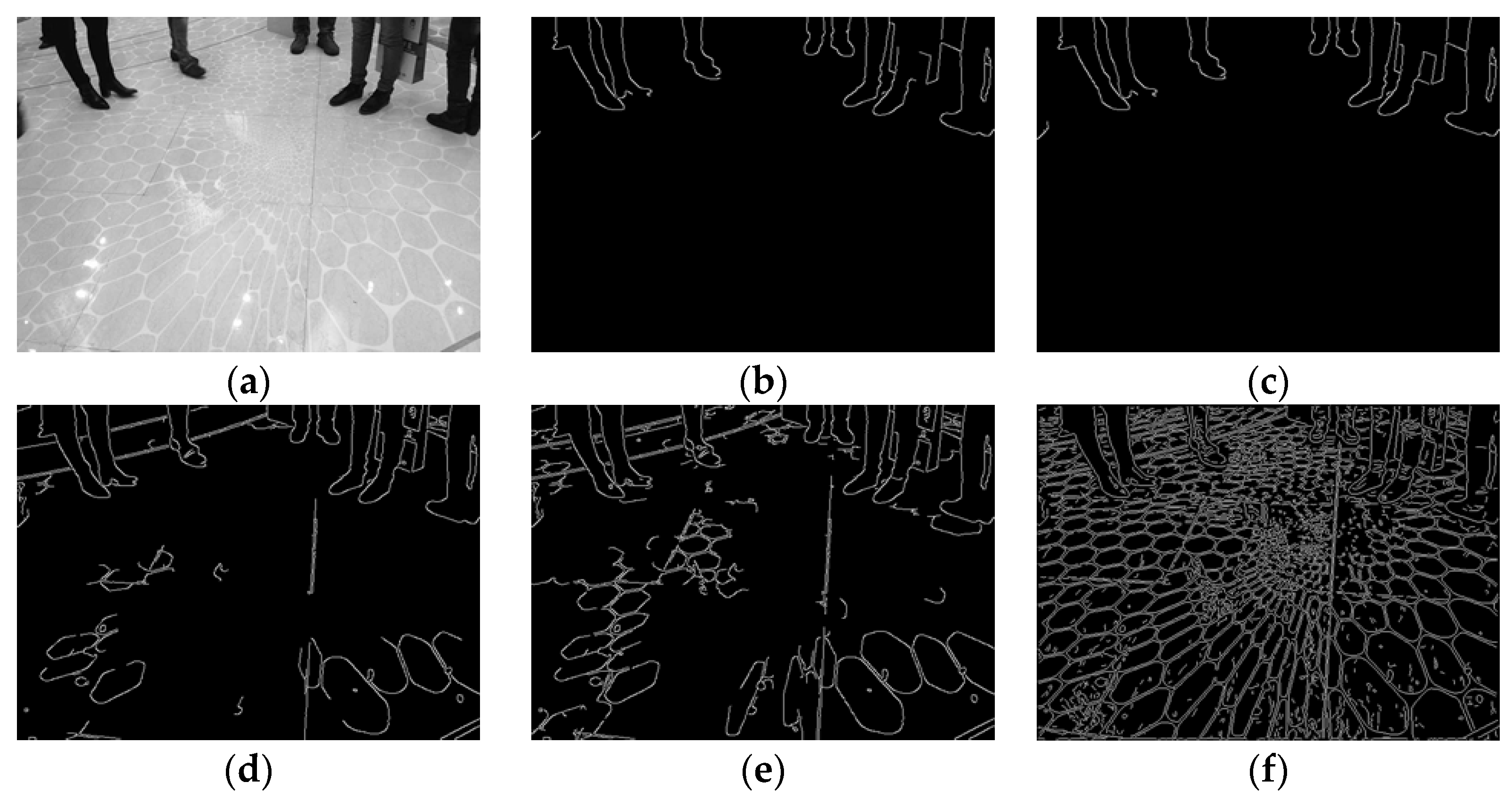
To show that TCEDA can detect more edge information than other edge detection methods, one of the experimental results of TCEDA is provided by referring to TCEDA [
28]. The TCEDA was compared with the other four improved adaptive Canny edge detection algorithms which were proposed by Gao and Liu [
29], Song et al. [
30], Saheba et al. [
31], and Li and Zhang [
32]. The results of the TCEDA compared with the other four improved adaptive Canny edge detection algorithms, as shown in
Figure 1.
Figure 1f shows the TCEDA can be effectively preserved the edge, the texture on the tile, the seam line between the tiles, and the wrinkles of the jeans.
Figure 2a,b is an image pair (Test image 1) obtained from the KITTI database [
34].
Figure 2a is the compared image (left image
IL) and
Figure 2b is the processing image (right image
IR). The edge image detected by TCEDA is shown in
Figure 2c. TCEDA can detect more edge information than other edge detection methods. However, some edge contours where image contrast is not clear may be detected incompletely, resulting in the fragmentation of line segments. This is analyzed and processed in the third processing step.
2.2. Distance Connected Component Algorithm
Because the edge image detected after being processed by TCEDA is pixel-wise information, the adjacent connected pixels should be labeled as the same line segment to obtain contour information of each line segment. Currently, the connected component labeling algorithm is the most widely used object labeling method. When objects with different distances overlap within the image, the connected objects will be labeled incorrectly owing to the adjacency edge pixels of the overlapping objects, and different overlapping objects will be labeled as the same object. Therefore, this paper proposes a distance connected component algorithm that combines the distance information of stereo vision and the characteristic of adjacent pixels and uses 3D information to label the edge image with different distances as different objects, thereby solving the labeling problem of overlapping objects.
The distance connected component algorithm is mainly divided into three steps—distance calculation, ground edge contour removal, and distance object labeling. During distance calculation, the edge pixels of the edge image are used as the processing pixels, and the image matching method is used to compare the displacement between
IR and
IL, and calculate the disparity value which represents the distance to the camera. The larger the disparity value, the closer the distance to the camera; the opposite is true. As shown in
Figure 3, we assume that there is a point
P in the space, and its positions in the images of the left and right cameras are
Pl (
ul,
vl) and
Pr (
ur,
vr), respectively. The disparity value
d can be obtained using Equation (1). Subsequently, the distance to the camera can be calculated using Equation (2), where
Z is the distance from point
P to the camera,
B is the distance between the two cameras, and
f is the focal length.
The block matching method is commonly used for image comparison. It calculates the difference in the gray level or color of the images in the two blocks within the search area. The smaller the difference, the higher the similarity between the two blocks. However, the images captured by different cameras are different in brightness and color, thereby affecting the accuracy of block matching. Therefore, this paper proposes a gradient weight comparison method, which replaces the pixel value with the gradient amplitude, and assigns different weights
ρ to the edge and non-edge pixels to improve the accuracy of block matching. Each edge pixel in the edge image of
IR is defined as the center point and extends a block image of
n ×
n pixels. The difference in gradient amplitude
GD(
u′,
v′) of each matched block in the search area
SA of
IL is calculated in sequence, as shown in Equation (3), where
GR(
x,
y) and
GL(
x,
y) are the gradient values of each pixel in
IR and
IL, respectively, the weight value of the edge pixels is 5, and the weight value of other pixels is 1. As shown in Equation (4), we identify the displacement coordinates (
u,
v) with the smallest weighted gradient amplitude difference in the search area. Then, we use Equations (1) and (2) to calculate
d and
Z, respectively.
where
and
is the search set and
R is an integer that determines the search area.
Then, ground edge contour removal is performed to avoid improper merging of edge contours in places where the object is in contact with the ground. First, the V-disparity method [
35] is used to produce a projection map of the calculated disparity values of all edge pixels, as shown in
Figure 4a, where the d-axis represents the change in disparity value and the v-axis represents the vertical coordinate of the image. The V-disparity map summarizes the change in disparity value of edge pixels in each row along the v-axis. If there is an edge contour of the ground, there will be a distribution of oblique line segments on the V-disparity map. Then, the Hough Transform [
36] is used to analyze whether there are oblique line segments in the V-disparity map. If there are oblique line segments, the edge pixels distributed in this area are deleted. The red line shown in
Figure 4b is the longest oblique line segment detected.
Figure 4c is the edge image after the ground is removed, and the edge contours of some objects in contact with the ground (e.g., a car tire, signal pole, and telegraph pole base) are also filtered out. Although there will be a small error in the height measurement of the object, the reduction of these edge contours does not affect the subsequent object segmentation.
Finally, distance object labeling is performed. Each edge pixel is considered as the center pixel in the order of raster-scan and determines whether there are adjacent edge pixels in four adjacent positions, that is, the left, upper left, upper, and upper right of the center pixel. If there is no adjacent edge pixel or the absolute value of the difference in distance between the center pixel and all adjacent edge pixels is greater than the preset distance threshold (TH_dis), a new label number is assigned to the center pixel and records it in the object-label array. If the absolute value of the difference in distance between the center pixel and adjacent edge pixel is less than or equal to TH_dis, the adjacent edge pixel with the smallest absolute value of the difference in distance to the center pixel is considered as the reference point, assign the same label number to the center pixel and the reference point, calculate the absolute value of the difference in distance between this reference point and other adjacent edge pixels, and change the label number of adjacent edge pixels with a distance less than or equal to TH_dis to the same label number as the reference point. During distance object labeling, the object-label array is used to store the label number and connection relationship of each object. When the label number of the adjacent edge pixel is modified, different objects are connected. Therefore, the object-label array is updated simultaneously to ensure that each object is connected correctly.
The setting of the distance threshold,
TH_dis, is automatically adjusted. Based on the parameters provided by KITTI (the relevant parameters will be explained in detail in the experimental results section), the change in the disparity value of one pixel at a distance of approximately 5 m and 20 m is converted to a distance change of 7 cm and 113 cm, respectively. This shows that the same disparity change has different resolutions at different distances. If the continuity of the disparity is directly used to determine the connection of adjacent pixels, the discontinuity of the disparity value of adjacent pixels will lead to misjudgment of the connection at close range. Therefore, this paper proposes an equation to automatically set the distance threshold. The
TH_dis is set based on the parameters related to the camera system. The distance resolution Δ
Z of the center pixel and the magnitude of the separation distance
S are used to determine the value of
TH_dis. The distance resolution Δ
Z can be expressed by Equation (5), where
d represents the disparity value of the center pixel. The value of
TH_dis is set using Equation (6).
The separation distance S is a preset fixed value, which is used to define the minimum distance between the overlapping objects to be segmented. Considering the difference in size and distribution of the objects photographed in outdoor and indoor scenes, this paper preset S to 30 cm and 10 cm for outdoor and indoor scenes, respectively.
The outdoor test image shown in
Figure 4c is used as an example to illustrate the process of distance object labeling. In the outdoor scene,
S is preset to 30 cm. In
Figure 5a, each grid represents the position of a single pixel, the number at the top of the grid is the distance (cm) of the pixel, and the number in the bracket at the bottom of the grid represents the label number. The parity value
d of the center pixel is 75 pixels, and the distance value is 515 cm computed by Equation (2). The Δ
Z obtained using Equation (5) is 7 cm. The
TH_dis is determined by Equation (6) to be 30 cm. First, the absolute value of the difference in distance between the adjacent edge pixels and the center pixel is calculated. Only the value of the upper left adjacent edge pixel is larger than
TH_dis, and the remaining are smaller than
TH_dis. Therefore, the upper left adjacent edge pixel is not adjusted, as shown in
Figure 5b. Next, we observed that the difference in distance between the center pixel and the upper right adjacent edge pixel is the smallest. Therefore, the label number of the center pixel is marked as (2), and the upper right adjacent edge pixel is defined as the reference point. Because the absolute value of the difference in distance between the upper adjacent edge pixel and the reference point is greater than
TH_dis, the upper adjacent pixel is not adjusted. The absolute value of the difference in distance between the left adjacent edge pixel and the reference point is less than
TH_dis; therefore, the label number of the left adjacent pixel is adjusted to (2). The processing result is shown in
Figure 5c.
After completing the distance connected component algorithm, each line segment can be labeled and recorded with 3D adjacent connection characteristics. The processing result of the distance connected component algorithm is shown in
Figure 6. In
Figure 6, different colors represent different line segments. Each line segment records the object number, bounding box coordinates, and endpoint coordinates. There are 4073 objects after the processing of the distance connected component algorithm, including single isolated points and line segments composed of multiple points.
2.3. Object Extension and Merge Algorithm
After the distance connected component algorithm is implemented, most of the object contours have fragmented problems. Therefore, the object extension and merge algorithm is used to extend and connect the fragmented line segments of the same object contour to obtain a more complete object contour as the boundary of subsequent object segmentation. The object extension and merge algorithm is composed of isolated point connection, single-distance plane line segment extension, and cross-distance plane line segment extension. The isolated point connection is used to solve the fragmentation problem of line segments caused by isolated points, and other line segment fragmentation problems are solved in the other two steps.
The isolated point connection places the result of the distance connected object on a 2D plane, fetches isolated points in sequence, and uses the isolated point as the center to find whether there are other objects in the adjacent points in the 3 × 3 block. If there is only one adjacent point, the isolated point is located at the endpoint of the line segment and can be directly merged with the adjacent point. If there are two adjacent points, the isolated point is in the middle of the line segment or the overlapping area of different object contours. In this case, we need to determine the difference in distance between adjacent points. When the difference in distance of two adjacent points is less than
TH_dis, the isolated point is merged with the two adjacent points. When the difference in distance is greater than
TH_dis, the isolated point is deleted. As shown in
Figure 7a, there are 1435 red points, which are isolated points.
Figure 7b shows the result of isolated point connection, that is, 4073 objects are merged into 2663 objects.
Subsequently, the single-distance plane line segment extension is processed to merge the fragmented line segments. The single-distance plane line segment extension mainly focuses on the line segments that are classified to the same distance plane and merges line segments that meet the extension connection condition. Before the processing, all objects should be arranged into planes with different distances based on the distance of objects. The minimum distance between the two endpoints of the line segment in each object is defined as the object distance. Therefore, objects with endpoints of the same minimum distance are classified into the same distance plane. Then, the line segment extension is processed for each distance plane in sequence. Because the object distances are calculated by Equation (2), the number of disparities will decide the number of distance planes. In
Figure 7b, the range of the disparities is from 1 to 80. Therefore,
Figure 7b can be classified into 80 distance planes. All objects in
Figure 7b are classified based on the object distances. As shown in
Figure 8a, 2663 objects are classified into 80 distance planes, where all planes are arranged in sequence. That is, Plane 1 is the closest plane, Plane 2 is the second plane, and Plane 80 is the farthest plane. We use the object in Plane 62 as an example and zoom in on the object for illustration, as shown in
Figure 8b. In the figure, different colors represent different contour line segments. This object is a truck, and its body and the shooting position have different distance values. Therefore, only the edge contour of the front of the truck is in Plane 62, and the other contours of the body are classified into different distance planes. It can be observed from
Figure 8b that the line segments of the front of the truck have fragmentation problems. The line segments can be extended and merged in this process.
The single-distance plane line segment extension comprises three processing steps, extension object search, extension connection judgment, and overlapping object processing. The first step is extension object search. The extension object search is sequentially to search whether the line segment endpoints of each object have extension objects in the extension direction in the same distance plane. The extension direction refers to the direction of the vector from the endpoint through the adjacent point, which can be divided into eight directions, as shown in
Figure 9. Searching the extended area of the perpendicular line at the endpoint of the extension direction. If no object exists, we do not perform the extension connection judgment but process the next object. If the object exists, these objects are defined as extension objects and perform the extension connection judgment.
The second step is to perform extension connection judgment in which two characteristics of a line segment, the closure property, and color continuity, are used to determine whether to extend and connect the endpoints of two different objects. The closure property of a line segment defines whether the extension of the line segment endpoints of two different objects can form the same line segment. The extension and intersection of two-line segment endpoints can be classified into two categories: (1) there is an intersection in the extension direction of the two endpoints; (2) the extension of a single endpoint intersects with another line segment. Plane 62 in
Figure 8 is used as an example, as shown in
Figure 10. The examples of Categories 1 and 2 are shown in
Figure 10a,b, respectively. Only the extension and intersection of the line segment endpoints in Category 1 can form the same line segment and satisfy the closure property.
The extension objects that satisfy the closure property of a line segment have to judge the color continuity of the line segment. In the process of color continuity, the similarity of the average color values on both sides of the line segment endpoints is compared between the processed object and the extension object. The method for calculating the average color value on both sides of the line segment endpoints is illustrated in
Figure 11. In the figure, the line segment is numbered sequentially from the endpoint, and a 7 × 7-pixel block centered on the 5th point (No. 5) of the line segment end point (No. 1) is obtained. In the pixel block, the line segment is used as the boundary line to calculate the average color value on both sides of the line segment and then obtain the sum of the absolute difference between the average color values of two object endpoints and both sides. If there are multiple extension objects, the smallest value of the sum of the absolute difference is used. When the sum of the absolute difference is less than
TH_color, object extension and merging are performed.
TH_color is preset to 60. During the object extension and merging, the label number of the extension object is changed to be the same as that of the processed object, the record of two extended and connected endpoints is canceled, the labeling data of the two objects are retained, and the bounding box coordinate record of the merged object is modified. Continuing to process the next object until all objects in this distance plane are processed.
Figure 12a shows the extension connection judgment result of Plane 62 in
Figure 8b. After the extension connection judgment, each object is composed of different line segments. Therefore, the third step, that is, overlapping object processing, is performed to merge different line segments of the same object on a single distance plane into the same object. The line segments are merged based on the overlapping characteristic of adjacent objects. Hence, the adjacent objects with overlapping bounding boxes are merged and the label number of the small object is changed to be the same as that of the large object. The bounding box coordinate record of the merged object is modified and the endpoint record of the two objects is retained.
Figure 12b shows the result of
Figure 12a after overlapping object processing. Different contour line segments of the front of the truck can be merged into the same object.
Figure 12c shows the processing result of the single-distance plane line segment extension. Here, 2663 objects are merged into 1146 objects after the single-distance plane line segment extension.
Finally, the cross-distance plane line segment extension is performed, and the main purpose is to judge each edge line segment in different distance planes and merge the line segments that satisfy the cross-plane extension connection condition. During the cross-distance plane line segment extension, planes are processed from nearest to farthest. First, all the endpoints of an object in Plane 1 are obtained and it is determined sequentially whether an extension object exists in Plane 2 in the extension direction of each endpoint. If there is no extension object, continue to process the next object of Plane 1. If an extension object exists, the extension connection judgment is performed based on the two characteristics of a line segment, the closure property, and color continuity. Finally, the extension object with the line segment closure property and line segment color continuity in Plane 2 is extended and merged with the object in Plane 1. The label number of the extension object in Plane 2 is changed to be the same as that of the merged object in Plane 1. The record of the two extended and connected endpoints is canceled, the bounding box coordinate record of the merged object is modified, and the labeling data of the two objects are retained. Then, repeating the above process of cross-distance plane line segment extension using Plane 3 and the merged plane of Planes 1 and 2 until all the planes are processed.
Figure 13 shows the result of the cross-distance plane line segment extension. Here, 1146 objects are merged into 821 objects after the cross-distance plane line segment extension.
It can be observed from
Figure 13 that large amounts of background noise are retained. The general practice is to set a threshold to filter the objects with a small number of pixels; however, the size of the same object in the 2D image is different at different distances. Therefore, the filtering method may incorrectly filter out distant objects. The proposed algorithm uses the 3D information of an object to determine whether to retain the object, to eliminate the object filtering error. In the proposed algorithm, two predefined thresholds are provided to filter out the noises. The two thresholds are the maximum detection distance and minimum reserved area. The objects with a distance less than the maximum detection distance and an area larger than the minimum reserved area are retained as the foreground objects, and the rest belong to the background image. In the experiments, the disparity value used as the maximum distance for effective detection is set as 5, and the distance calculated by Equation (2) is the maximum detection distance. Considering the retained object size is different for indoor and outdoor, the minimum reserved area of indoor and outdoor scenes is set to 25 cm
2 and 600 cm
2, respectively. Based on the relevant parameters of the KITTI camera system, the calculated maximum detection distance threshold is 77.3 m, and the minimum reserved area is 600 cm
2. There are originally 821 objects, as shown in
Figure 13. After the threshold filtering, 16 foreground objects are retained, as shown in
Figure 14.
2.4. Object Segmentation
Object segmentation is performed to segment the foreground objects from the image for subsequent image recognition. The 3D information of the objects can also be used as an auxiliary parameter for object recognition. The objects processed by the object extension and merge algorithm only have the information of the contour line segments. Therefore, morphology closing is used to perform dilation and erosion on the contour line segments of each object to convert the contour line segments into a closed region. When a gap exists within the closed region after the morphology closing, the run-length smoothing algorithm [
37] can be used to fill the gap in the closed area to obtain a solid region for subsequent object segmentation.
Figure 15 shows the result after object segmentation. Analysis of the segmented objects will be explained in the subsequent section.
3. Experimental Results
To verify the practicality of the proposed algorithm, the test images from the KITTI dataset [
34] for outdoor scenes, and test images from the Middlebury dataset [
38] for indoor scenes are used. Because the KITTI and Middlebury test images do not provide the distance and size of objects in the images, a dual-camera system is made to capture indoor and outdoor images and measured the actual distance and size of objects in the images to verify the estimated data of the proposed algorithm. The overall accuracy (
OA) [
39] is used to compare the accuracy of the segmented objects with the ground truths in this paper. The
OA is defined as Equation (7), where the
TP,
TN,
FP, and
NT are true positive, true negative, false positive, and false negative, respectively.
The proposed algorithm uses Visual C++ 2015 for programming. In addition to the disparity value of the image pair, the distance calculation for stereo vision required relevant hardware parameters, such as baseline, focal length, sensor size, and image resolution. The relevant parameters will be explained in the subsequent experimental results.
The KITTI dataset includes images captured by vehicles driving on outdoor roads. The Point Gray Flea2 color cameras (FL2-14S3C-C) and the 1/2″ Sony ICX267 CCD sensor are adopted. The focal length is 4 mm, and the baseline is 54 cm. The first test image pair selected from the KITTI database is Test image 1, as shown in
Figure 2a,b. The image resolution is 1242 × 375 pixels. Regarding related parameters, the maximum detection distance is 77.3 m, the separation distance is 30 cm, and the minimum reserved area is 600 cm
2.
Figure 15 shows the foreground objects segmented by the proposed algorithm. After foreground object segmentation, the remaining image is the background image, as shown in
Figure 16.
Sixteen different objects are segmented in Test image 1. Then, based on the label number of each foreground object in
Figure 15, the foreground objects are sequentially segmented from the image and estimated the distance and size of the objects. For size estimation, the width is defined as the difference in distance between the leftmost and rightmost contour pixels within the bounding box of each object, and the height is defined as the difference in distance between the top and bottom contour pixels. The object distance is defined as the minimum distance value of all contour pixels of the foreground object.
Table 1 lists the relevant segmentation results and 3D information, including the segmentation result, distance, and size of the foreground object. Because ground removal also removed the contour of the foreground object in contact with the ground, the object height is slightly reduced. For example, for objects 5, 8, and 16, the calculated heights of the vehicles are lower. From the results of Test image 1, it can be observed that objects with different distances and overlapping objects can be effectively detected and segmented. These segmented objects are suitable for the input of subsequent image recognition, and the object size information can be used as an important reference.
The second set of test images selected from KITTI is Test image 2, which is an outdoor scene beside the road. The experimental results of Test image 2 are shown in
Figure 17.
Figure 17a is the image pair. The image resolution is 1224 × 370 pixels, and the hardware parameters and the threshold values used by the algorithm are the same as those of Test image 1.
Figure 17b is the detection result of the object edge contour. The object segmentation result is shown in
Figure 17c, and the remaining image is the background image, as shown in
Figure 17d. A total of 14 different foreground objects are detected and segmented from Test image 2.
The distance and size of the foreground objects are estimated by the proposed algorithm and are listed in the sequence in
Table 2. Fourteen foreground objects, as shown in
Figure 17c, can be observed that there are five complex overlapping objects, that is, objects 2, 3, 4, 5, and 7, below object 1. The proposed algorithm can effectively detect and segment each object and estimate the distance and size of the object. The rightmost plane of object 1 had interference from the shadow of the leaves. Because the proposed algorithm used distance as an important reference for the contour connection and adjacent extension, the result of
Figure 17b shows that the contour line segment of the object 1, the building, is not affected by the shadow of leaves in the image, and the contour of the object 1 is effectively constructed. In addition, objects 6 and 8 are on the upper right and right sides of object 1, respectively. From the original image, it can be observed by the naked eye that object 6 appeared to be an extension of the leaves with object 8. However, it can be observed from
Table 2 that the distances of objects 1, 6, and 8 are 15.46 m, 29.73 m, and 11.04 m, respectively. Based on the distance of the objects, we can realize that object 8 is the tree in front of object 1, and object 6 is another tree behind object 1. Therefore, the proposed algorithm can effectively avoid the misjudgment of 2D images.
The Middlebury dataset includes test images captured in indoor scenes by Canon DSLR cameras (EOS 450D). The focal length and baseline are different for each set of the test images, and the provided focal length is converted to the pixel unit of each image. The first set of test images selected from the Middlebury dataset is Test image 3. The experimental results of Test image 3 are shown in
Figure 18.
Figure 18a is the image pair. The image resolution is 2964 × 2000 pixels, the focal length is 3979.911 pixels, and the baseline is 193.001 mm. Regarding relevant parameters, the maximum detection distance is 5.9 m, the separation distance is 10 cm, and the minimum reserved area is 25 cm
2.
Figure 18b shows the segmentation result of the object edge contour. The object segmentation result is shown in
Figure 18c. The background image is shown in
Figure 18d.
Four different foreground objects are detected and segmented from Test image 3 shown in
Figure 18c. The distance and size of the foreground objects are estimated and listed in the sequence in
Table 3. From the segmentation results of Test image 3, it can be observed that the complex overlapping objects, that is, objects 1, 2, and 3, can be effectively segmented.
The second set of images in the Middlebury dataset is Test image 4. The experimental results of Test image 4 are shown in
Figure 19.
Figure 19a is the image pair. The image resolution is 1920 × 1080 pixels, the focal length is 1758.23 pixels, and the baseline is 97.99 mm. The maximum detection distance is 43.9 m, the separation distance is 10 cm, and the minimum reserved area is 25 cm
2.
Figure 19b shows the detection result of the object edge contour. The object segmentation result is shown in
Figure 19c. The background image is shown in
Figure 19d.
Three different foreground objects are detected and segmented from Test image 4 shown in
Figure 19c. The distance and size of the foreground objects are estimated and listed in the sequence in
Table 4. Because the object segmentation uses morphology closing and run-length smoothing algorithm to label the region covered by the object, the hollow area inside the object is also labeled as part of the object. Considering object 1 in
Table 4 as an example, we observe that the hollow area of the chair is directly labeled as part of the object, and this did not affect the subsequent analysis and recognition of the object.
Because the above Middlebury and KITTI datasets did not provide the distance or the size of each object, this paper develops an image capture system to capture test images, as shown in
Figure 20. Two Diamond color cameras (15-CAH22) are used, and the image capture card is an ADLINK PCIe-2602. The relevant hardware specifications are as follows: the sensor is a 1/3″ Panasonic CMOS, the image resolution is 1920 × 1080 pixels, the camera pixel size is 2.5 μm × 3.2 μm, and the focal length is 6 mm. Considering that the distance of the objects to be photographed in indoor and outdoor scenes is different, the baseline of the two cameras is designed to be adjustable. In
Figure 20, the camera on the left is fixed. The camera on the right is controlled and adjusted to the desired position by the stepper motor, and the adjustable range is from 0–45 cm. In this paper, the baseline is a preset fixed value for outdoor or indoor scenes. Therefore, only two baselines are adjusted by the preset rotation angles of the stepper motor. The baseline of the outdoor or indoor is set to 300 mm or 50 mm, respectively.
Test image 5 photographed by the self-made image capture system is an outdoor test image. The experimental results of Test image 5 are shown in
Figure 21.
Figure 21a is the image pair of Test image 5. The baseline is set to 300 mm. The rest of the hardware specifications are described in the previous paragraph. Regarding relevant parameters, the maximum detection distance is 40 m, the separation distance is 30 cm, and the minimum reserved area is 600 cm
2.
Figure 21b shows the detection result of each object contour. The object segmentation result is shown in
Figure 21c. The background image is shown in
Figure 21d. A total of 16 different foreground objects are segmented from Test image 5.
The distance and size of the foreground objects are estimated by the proposed algorithm and are listed in the sequence in
Table 5. It can be observed from the experimental results that the complex overlapping objects in the image can be effectively detected and segmented. For example, objects 9 to 12 are complex overlapping objects. These objects, from closest to furthest, are Person A, Person B, streetlamp, and coconut tree. All foreground objects can be effectively detected and segmented. Because the ground contour is detected, part of the contour of the object in contact with the ground is removed and the estimated height of the object is slightly lower.
For the test image captured by the self-made camera system, we can measure the actual distance and size of the objects in the image using measuring tools. Considering that the plant size is affected by the wind and subjective judgment, we only measure the distance of the plant. The actual measurement of the objects and the object information estimated by the algorithm are listed in
Table 6. It can be observed from
Table 6 that although the self-made camera system did not perform stereo rectification, the distance and size of the object estimated by the algorithm could be used as effective references for determining the actual distance and size of the object.
Test image 6 photographed by the self-made image capture system is an indoor test image. The experimental results of Test image 6 are shown in
Figure 22.
Figure 22a is the image pair of Test image 6. The baseline is set to 50 mm. The rest of the hardware specifications are the same as those for Test image 5. Regarding relevant parameters, the maximum detection distance is 4.5 m, the separation distance is 10 cm, and the minimum reserved area is 25 cm
2.
Figure 22b shows the detection result of the object contour. The object segmentation result is shown in
Figure 22c. The background image is shown in
Figure 22d. A total of 13 different foreground objects are detected and segmented from Test image 6.
Thirteen foreground objects, as shown in
Figure 22c, are segmented from Test image 6. The distance and size of the foreground objects are estimated by the proposed algorithm, which are listed in the sequence in
Table 7. From the experimental results, it can be observed that the complex overlapping objects in the image can be effectively detected and segmented.
The actual measurement of the objects and the object information estimated by the proposed algorithm are listed in
Table 8. Because the baseline used in the indoor scenes is short, the estimated object information for indoor objects is relatively close to the actual measured data.
From
Table 6 and
Table 8, the results for the height seem to be more accurate than for the width. According to our careful analysis of the reasons, we find there are two causes to affect the accuracy of the measured size. The two causes are the detection error and the oblique problem. The detection error occurs when the detected pixel number of the height or width is incorrect. When the detection error occurs, the oblique problem of the object will influence the accuracy of the measured width seriously. In this paper, we define a distance resolution Δ
Z to represent the difference in depth when the disparity value only changes one pixel under different distances. The value of Δ
Z is increased when the distance of the object is away from the cameras. When the object plane is not parallel to the image plane, the distance resolutions of the two sides of the width are different and the far side will cause more error. Therefore, the oblique problem will increase the detection error for measuring the width of an object.
The proposed algorithm has been processed by a computer with an Intel Core i7-6700 CPU, 16 G RAM, and NVIDIA GeForce GTX 1080 GPU with 8 GB memory. The software has not been optimized. The processing times of the test images are shown in
Table 9. The processing time will vary according to the image resolution. We believe the proposed algorithm can be used for real-world applications.


