Compliant Cross-Axis Joints: A Tailoring Displacement Range Approach via Lattice Flexures and Machine Learning

Abstract

Compliant joints are flexible elements that allow displacement due to the elastic deformations they experience under the action of external loading. The flexible parts responsible for these displacements are known as flexure hinges. Displacement, or motion range, in compliant joints depends on the stiffness of the flexure hinges and can be tailored through various parameters, including the overall dimensions, the base material, and the distribution within the hinge. Considering the distribution, we propose the stiffness modification of a compliant cross-axis joint via the use of lattice mechanical metamaterials. Due to the wide range of parameters that influence the stiffness of a lattice, different machine learning algorithms (artificial neural networks, support vector machine, and Gaussian progress regression) were proposed to forecast these parameters. Here, the machine learning algorithm with the best forecasting was the Gaussian progress regression; this algorithm has the advantage of well-tuning even with small regression databases, allowing these functions to more easily adjust to suit specific data, even if the dataset is small. Hexagonal, re-entrant, and square lattices were studied as flexure hinges. For each, the effect of the unit cell size and its orientation with respect to the principal axis on the effective stiffness were studied via computational and laboratory experiments on additively manufactured samples. Finite element predictions resulted in good agreement with the experimentally obtained data. As a result, using lattice-flexure hinges led to increments in displacement ranging from double to ten times those obtained with solid hinges. The most suitable machine learning algorithm was the Gaussian progress regression, with a maximum error of 0.12% when compared to the finite element analysis results.

1. Introduction

In recent years, the implementation of new technologies such as additive manufacturing (AM) has helped engineers to expand the field of knowledge in a vast array of mechanical areas. Among these, highlight compliant mechanisms or joints (CJs) and mechanical metamaterials or cellular materials, which have had a significant impact on the innovation of new mechanical applications. On the other hand, the development of specialized algorithms has helped in the automation of specific mechanical applications. This is the case for machine learning (ML) algorithms that have been used in mechanical applications as a tool to forecast performance and/or in the selection of design and manufacturing parameters to achieve specific properties.

1.1. Compliant Joints and Their Applications

A CJ is a mechanical joint encountered in compliant mechanisms (CM) that allows motion due to the elastic displacement of their flexible parts, known as flexure hinges (FHs). In other words, compliant joints are the key components in compliant mechanisms; they act analogously to the kinematic pairs in rigid-body mechanisms [1]. Thanks to the use of different types of CJs, many applications have appeared, including in specific areas of mechanical engineering such as robotics [2,3,4,5] and micro-electromechanical systems (MEMSs) [6,7,8,9]. In robotics, the use of CJs has grown significantly, reflected in the design of complex mechanisms and robots. That was the case for Hoover and Fearing, whose main objective was to improve the performance of a compliant Sarrus linkage by means of topological linkage modification [10]. Another example of this growth was presented by Tummala et al.; their work was an implementation of a compliant spine for a flapping wing in unmanned aerial vehicles, with the goals of weight reduction and the relief of stress on the component [11]. Additionally, other works where the main objective was the development of optimal robotic members are also reported in the literature. For example, a three-degrees-of-freedom robotic arm with compliant fingers [12], the design of a compliant finger for a 3D endoskeleton with soft matter [13], the development of an engineering method for quantifying the CJ compliance of robotic hands [14], and the design of soft monolithic robotic fingers for prosthetic hands [5]. In the field of MEMSs, CJs have been widely used and tested, resulting in progress for medical devices and precision engineering applications. In medicine, MEMSs have been used for surgical implementations [15], such as in intraocular surgeries [16] and biomedical executions [17]. In the case of precision engineering applications, MEMSs have been explored for use as flow sensors [8] and for consumer product applications where IC-based technology tends to fail [9].

The range of motion that a CJ can achieve depends on the stiffness of its flexures, which in turn depend on the external geometry, dimensions, and base material used. In order to widen the range of applications for CJs, researchers have explored different approaches to tailoring their stiffness, as recently reviewed by Arredondo-Soto et al. [1]. With the aim of reducing stiffness (increasing motion range) in CJs, Merriam and Howell [18] explored the use of lattice structures. In [18], the implementation of mechanical metamaterials as lattice flexures instead of blade flexures was studied. This study concluded that lattice flexures could achieve reductions in bending stiffness in the range of 60 to 80% compared to fully solid blade flexures of the same size. The lattice-compliant joints studied in [18] were additively manufactured.

1.2. Mechanical Metamaterials and Their Applications

A mechanical metamaterial is a material created artificially with specific characteristics adjusted by the designer to suit particular tasks. The mechanical properties of metamaterials come from their microstructural geometries rather than their material constitution [19]. Mechanical metamaterials are often porous and formed from the repetition of the basic unit known as the unit cell. Their porosity may be encountered in 2D or 3D. The effective mechanical properties of metamaterials are tailored via the controlled distribution of matter within a structure. These controlled arrangements often result in periodic structures and can be defined through effective or apparent properties, which depend on the topology, volume fraction, and base material. The field of mechanical metamaterials has also benefited from the growth of additive manufacturing technologies, as these allow the fabrication of porous structures with complex geometries [20]. In engineering, the three relevant elastic metamaterial properties are stiffness, rigidity, and compressibility [19]. Mechanical metamaterials can be found in various engineering applications, including biomedicine and the aerospace and automobile industries.

In biomedicine, for example, the use of mechanical metamaterials as bone implants has been explored, along with the understanding of the effects of bone formation during early osteointegration [21]. In addition, biomedical applications such as new techniques for the development of tissue engineering scaffolds for cell culture studies [22] and the implementation of hybrid meta-biomaterials for tissue regeneration [23] have been investigated.

In the aerospace and automobile industries, many applications have been developed over the years to innovate the design of specific components. For example, for aerospace engineering, auxetic (negative Poisson’s ratio) composites and materials have been tested due to their high shear modulus and damping resistance [24]. The term auxetic was first used by Evans et al. [25] in 1991, and it comes from the Greek word auxetikos, which means something that tends to increase [26]. Other topologies that have been shown to have auxetic properties are those based on chirality or achirality. They were used by Spadoni et al., who proposed a method for the implementation of chiral topologies in wing airfoils [27]. Another example is the one proposed by Mizzi et al., where the use of hierarchical truss elements as mechanical metamaterials was explored to develop lightweight aerospace components [28]. In the field of motor vehicles, Scarpa et al. worked with auxetic structures in vibration-damping bodies for Rolls-Royce automobiles [29].

1.3. Machine Learning Applications in Mechanics

Artificial intelligence (AI), specifically ML, has become an important area of study in the modern era. ML has a huge variety of applications that cover various fields of knowledge, and mechanical engineering is not an exception; applications of ML allow researchers to predict and/or classify specific mechanical properties. ML can also aid the manufacturing process by assisting in the selection of parameters for specific processes [30], allowing the automation of the design of some actuators [31]. The application of hybrid ML to select design parameters in modern mechanical applications, such as in mechanical metamaterials, has been reported [31,32,33,34,35]. Other applications of ML in the structural sector are found in the works of Fu et al. [36,37], where the weighted averaging of non-fine-tuned ML models was applied to the concrete construction sector, with special emphasis on corroded beams.

ML has been tested in the field of mechanical metamaterials to forecast specific mechanical properties and reduce iterations in the design processes. In this form, an ML algorithm can be used to predict errors in compliant auxetic designs based on a mathematically optimal deformation [32]. Another manner of using ML in the field of mechanical metamaterials is to aid in the design process to obtain smart structures with programmable mechanical responses [34]. In the work of Bessa et al., this approach was presented, and it included the generation of a new metamaterial that can be designed and adapted to different target properties by the implementation of Bayesian ML [35]. In addition, ML has been used with trained datasets to automate specific design processes concerning mechanical metamaterials. That was the case for Gu et al., who developed a method to design hierarchical materials using machine learning using a trained dataset with thousands of structures from finite element simulations [33].

With the aim of enhancing the displacement range in additively manufactured CJs and aiding their design process via ML, in this work, we study compliant cross-axis joints (CCAJs) where flexures have been replaced with lattice flexures. The stiffness of these FHs is modified using mechanical metamaterials as honeycomb lattices (hexagonal, re-entrant, and square). The resulting lattice-flexure hinges (LFHs) with different lattice topologies are studied both computationally and experimentally on additively manufactured samples. Finally, the use of ML is explored to aid in the selection of design and topology parameters to achieve specific elastic performance.

The remainder of the work is structured as follows: Section 2 includes all the details of the computational design process, parameter definitions, finite element modeling, additive manufacturing, and ML; Section 3 reports on the simulations and experimental results, along with a comparison with ML predictions; Section 4 presents discussions of how the stiffness generated in each LFH affected the displacement of the CCAJ, as well as the importance of identifying the deformation mechanisms in specific LFHs and understanding how they affect the total range of motion of CCAJs; finally, in Section 5, some important concluding remarks and an overview of future work are presented.

2. Materials and Methods

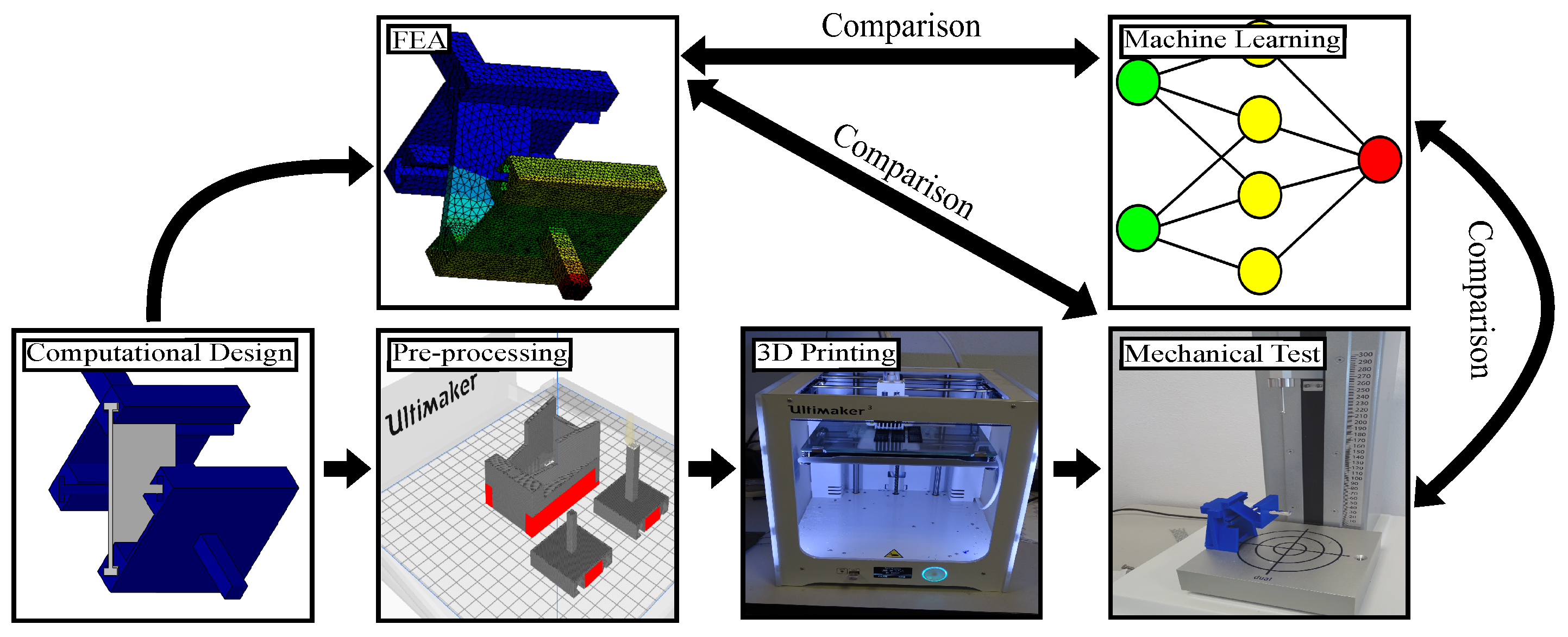
In this section, we outline the methodology followed, which consisted of 6 main steps: computational design, finite element modeling, pre-processing, 3D printing, mechanical tests, and ML implementation (Figure 1). For the computational design, the definition of the dimensions was the main goal. The next step was the finite element modeling that allowed the mechanical elastic simulation of each of the CCAJs proposed; then, the simulation results were used to generate a dataset for the prediction of specific mechanical parameters during the ML implementation. For pre-processing, the design of the final CCAJ was imported into the 3D-printing software to define the manufacturing parameters. The 3D-printing step allowed us to fabricate the models defined and calibrated in the pre-processing step. During this step, the tolerances of some parts were obtained in order for them to fit properly in the experimental setup assembly. Finally, once all the dimensions of the CCAJ were found, the mechanical tests were performed in order for the LFH configurations to be established.

2.1. Computational Design of Lattices and Compliant Cross-Axis Joints

The CCAJ was first proposed in [38]. Here, computational models for CCAJ and LFHS were built using Solidworks^® (v2019, Dassault Systèmes, Waltham, MA, USA). The macro-dimensions of the flexure hinges, shown in Figure 2a, were kept constant as follows: length (l) 42.23 mm, width (w) 20 mm, and depth 2 mm (e). The lattice honeycomb patterns studied here, i.e., re-entrant, hexagonal, and square, are shown in Figure 2b–d. To compare the mechanical responses, the representative unit cell dimensions (a) were adjusted to obtain close values for the volume fraction (relative density) among the different topologies. The values for a used were 5.5 mm for the re-entrant LFH and 3.5 mm for the hexagonal and square. Finally, for the internal unit cell dimensions, a constant thickness (t) of 0.5 mm was used. An internal angle (o) equal to 50° was used for the re-entrant lattice (Figure 2d). The resulting volume fractions used were 0.27, 0.30, and 0.32 for the square, hexagonal, and re-entrant, respectively. To study the effect of the lattice orientation with respect to the principal axis of the flexures, lattice arrangements were rotated to orientations from 0° to 80° with intervals of 20°. Examples of these for the re-entrant topology are depicted in Figure 3.

The complete CCAJ is shown in Figure 4, and it consisted of four main removable parts: a fixed add-in, a fixed part, two removable FHs or LFHs, and the acting part. The fixed part was designed to fit into a modified fixed add-in that was screwed into the base of the experimental setup (more details are given in the upcoming subsections). A “T” joining system was proposed to assemble the flexure to the fixed and acting parts. The acting part included a prismatic extension for the load to be applied. The part labeled as flexure hinges was replaced with the lattice hinges, resulting in a lattice-compliant cross-axis joint (LCCAJ). Samples here are labeled with the following scheme: lattice topology (RH for re-entrant, HH for hexagonal, and SH for square)-unit cell dimension a-orientation (°). Hence, a sample labeled as RH-5.5–80° is that corresponding to the re-entrant lattice with a unit cell dimension of 5.5 mm oriented at 80°.

2.2. Finite Element Modeling of Lattice-Compliant Cross-Axis Joints

A total of 15 LCCAJs were simulated in Ansys Workbench^®(Canonsburg, PA, USA). The material used for the simulations was polylactic acid (PLA) with a Young’s modulus of 2.35 GPa [39] and a Poisson’s ratio of 0.36 [39]. The finite element (FE) analyses were performed with a second-order mesh with linear tetrahedron elements in all cases. The sizings of the elements were 2 mm for the fixed and acting part and 0.5 to 1.5 mm for the LFHs. Boundary and loading conditions are shown in Figure 5. Fully fixed boundary conditions were applied to the fixed part. The loading was applied to the prismatic extension on the acting part, with a value of F = 0.04905 N (5 g). This load value was selected by inspection of the experimental results as it was within the linear elastic stage of the response of the samples. Additionally, contact pairs were set at the “T” joints.

2.3. Additive Manufacturing of Latticed Compliant Joints

All the designs were additively manufactured using fused deposition modeling (FDM) with an Ultimaker 3 3D printer. The pre-manufacturing process was performed in CURA^®v4.3.0 (Ultimaker B.V., Utretch, The Netherlands). Here, the “.stl” version of the models was processed considering the use of PLA as the printing material. For all the fixture elements, i.e., the “T” joints and the holes from the fixed add-in, tolerance tests were conducted several times until the final dimensions were found (Figure 6a). Printing support structures were needed for all the overhang parts, such as the “T” joint (Figure 6b). Once all the tolerances were obtained, the printing parameters for the parts of the CCAJ used were as follows: 0.3 mm layer height quality printing, 60 mm/s printing speed, 250 mm/s travel speed, 20 % infill density, and touching build plate support. The components printed for the CCAJ were the fixed add-in, the fixed part, and the acting part (Figure 6c). Printing orientations for all the parts fabricated are shown in Figure 6. The printing parameters for all the LFHs were as follows: 0.1 mm layer height quality printing, 60 mm/s printing speed, 250 mm/s travel speed, 20 % infill density, and build plate adhesion enabled (Figure 6d).

2.4. Experimental Mechanical Testing of Additively Manufactured Compliant Joints

The experimental mechanical tests were performed using a texturometer Perten TVT 6700 with the software TexCalc 5^® (v5.2.2.287, Perten Instruments, New South Wales, Australia), as shown in Figure 7. First, the fixed add-in of the LCCAJ was screwed to the base of texturometer on the left side of the main platform. Then, the fixed part with its corresponding LFH and the acting part were fastened to the fixed add-in. An example of the complete experimental setup is shown in Figure 7. Once all the components were secured, the testing machine was operated under displacement control, setting a maximum displacement of 10 mm downwards. The load was applied through a spherical probe with a diameter of 5 mm. The data for load displacement were exported and further processed in Matlab^® (R2021a, MathWorks, Natick, MA, USA).

2.5. Machine Learning Approach for the Prediction of Mechanical Properties

All ML algorithms were trained with a dataset that consisted of 105 data points obtained from FEA simulations. The aim was to forecast the displacement and stiffness with normal learning. In this dataset, all data were organized in 7 columns representing the following parameters: lattice topology, force (F), relative density, base material stiffness (Young’s modulus), lattice orientation, displacement ($\delta$), and compliant joint stiffness ($F/\delta$). For the forecast, the inputs defined were material, lattice orientation, volume fraction, lattice topology, and force, while the outputs selected were displacement and stiffness (Figure 8).

Supervised learning was implemented with a validation type of k-fold cross-validation for the dataset. Cross-validation is a technique that consists of a series of steps to measure the skills of the ML algorithm when new data are presented to it. The method randomly divides the dataset into k groups of the same size. This allows using part of the groups for training and testing; in this way, the ML algorithm was tested with data that had never been presented to it. The dataset was divided into k folds that represent the number of groups into which the dataset was divided, a classifier was trained using $k-1$ folds, and an error value was calculated by testing the classifier in the remaining fold [40]. The steps to estimate the tuning parameter $\lambda$ in k-fold cross-validation were:

1.

The data was divided into k roughly uniform parts.

2.

For each $k=1,2,\cdots K$, the model must fit with the parameter $\lambda$ in $K-1$ parts, resulting in ${\widehat{\beta }}^{-k}\left(\lambda \right)$ to finally compute the error in predicting the kth part:

$$E_k\left(\lambda \right)={\Sigma }_{i\in k\mathrm{th}part} {(y_i-x_i{\widehat{\beta }}^{-k}\left(\lambda \right))}^2$$

(1)

which gave the cross-validation error:

$$CV\left(\lambda \right)=\frac{1}{K}\sum _{k=1}^K{E}_k\left(\lambda \right)$$

(2)

3.

Then, this process was repeated for many values of $\lambda$ in order to find the value of $\lambda$ that made the CV($\lambda$) smallest. In this step, $K=5$ or 10 was used.

In this way, 4 to 5 random parts were occupied, and the weights of each corresponding parameter were used. During this normal learning method, multiple ML algorithms were implemented to compare and seek the learning algorithm that best fit the data. The objective was to predict the output values of the dataset and obtain the error margin by comparing the FEA results of the simulations with the predictions. In order to apply the ML algorithms, the ML module from Matlab^® was used. The learning algorithms used were artificial neural networks (ANNs), Gaussian process regression (GPR), and support vector machine (SVM).

For each of the algorithms, several parameters were established, depending on the variable, to predict and obtain a better response performance. First, the algorithms were calibrated based on the prediction of the displacement variable. In this case, for the ANN1, the model type was a medium neural network with just one fully connected layer, 25 sizes on the first layer, a ReLU activation function, and an iteration limit of 1000. For the ANN2, the model type was a wide neural network with just one fully connected layer, a 100 size on the first layer, a ReLU activation function, and an iteration limit of 1000. For the GPR, the model type was an optimizable GPR with a signal standard deviation of 0.23747, a Bayesian optimization, optimized hyperparameters with a sigma of 2.9764, a constant basis, and a non-isotropic squared exponential kernel function. For the SVM, the model type was a linear SVM with a linear kernel function. Finally, for the stiffness forecasting, the parameters varied except for the ANN1, where the same parameters were used. The model type of the ANN2 was a trilayered neural network with three fully connected layers and sizes of 10 for the first, second, and third layer, respectively; a ReLU activation function was applied, and an iteration limit of 1000 was established. For the GPR, the model type was an optimizable GPR with a signal standard deviation of 0.026359, a Bayesian optimization, optimized hyperparameters with a sigma of 0.23382, a constant basis function, and a non-isotropic exponential standardized kernel function. For the SVM, the model type was an optimizable SVM with a quadratic kernel function and optimized hyperparameters with an epsilon of 0.018356 and a Bayesian optimization.

3. Results

3.1. Additively Manufactured Lattice Flexures and Compliant Joints

Considering triplicates, a total of 150 samples of LFHs were printed to test in LCCAJs. As an example, some of LFHs printed for each topology are shown in Figure 9 for all three different orientations. The dimensions shown in Figure 9 (5.5 and 3.5 mm) correspond to the unit cell size a. On the other hand, the fixed add-in, the fixed part, and the acting part from the CCAJ were printed once and used in all tests. Examples of the complete assemblies of compliant joints with solid- and lattice flexures (re-entrant) are shown in Figure 10a,b, respectively. In some LFH samples, defects resulted from the removal of the supports. As seen in Figure 11, many extruded filaments (rasters) were detached irregularly while removing the supports.

3.2. Reducing Stiffness in Compliant Joints Via Lattice Flexures: Comparison between FEA and Experiments

A total of 75 tests using the LFHs with their respective lattice pattern topologies and a single test involving solid flexure hinges were performed. An example of a CCAJ under experimental loading during the test is shown in Figure 12a. This deformed shape obtained in the experiments was validated with FEA, for which an example is shown in Figure 12b. FE models were further used to predict the displacements of the CCAJs with LFHs. FEA predictions for the stiffness of each case were then compared with the experimental results. A comparison between FEA and experimental force-displacement curves is shown in Figure 13 for the stiffest and most flexible cases obtained for each lattice topology. The errors obtained from comparing FEA predictions and measurements of additively manufactured samples are listed in

Table 1. Comparison and error percentage (%E) for the measured average displacement and $F/\delta$ compared with those from FEA.

Average Experimental and FEA Displacement (mm) and F/$\delta$ (N/mm)
Lattice-Flexure	Displacement			F/$\delta$
Hinges	Experimental	FEA	%E	Experimental	FEA	%E
RH-5.5-0°	0.586	0.5789	1.2%	0.0856	0.0847	1.06%
RH-5.5-20°	0.854	0.7309	14.4%	0.0633	0.0671	6.08%
RH-5.5-40°	1.252	1.2002	4.14%	0.0434	0.0408	5.81%
RH-5.5-60°	1.318	1.4082	6.84%	0.0372	0.0348	6.45%
RH-5.5-80°	1.194	1.205	0.92%	0.0415	0.0407	1.95%
HH-3.5-0°	0.52	0.454	12.5%	0.1023	0.1078	5.36%
HH-3.5-20°	0.496	0.5064	2.09%	0.0993	0.0969	2.47%
HH-3.5-40°	0.558	0.5621	0.73%	0.0909	0.0872	4.01%
HH-3.5-60°	0.738	0.7496	1.57%	0.0688	0.0654	4.96%
HH-3.5-80°	0.898	1.031	14.81%	0.0554	0.0476	14.17%
SH-3.5-0°	0.304	0.2892	4.86%	0.1617	0.1696	4.86%
SH-3.5-20°	0.4968	0.4708	5.24%	0.1038	0.1042	0.41%
SH-3.5-40°	0.7434	0.7196	3.2%	0.0666	0.0682	2.27%
SH-3.5-60°	0.676	0.6402	5.29%	0.075	0.0766	2.19%
SH-3.5-80°	0.392	0.3624	7.55%	0.1298	0.1353	4.27%

.

Note that both the FEA stiffness predictions and the ML forecasting are included, with dotted lines, in Figure 13 (ML forecasting is discussed in an upcoming subsection). The stiffest values of the hexagonal LCCAJs were obtained for a configuration with a 3.5 mm unit cell and 0° lattice orientation (0.46 mm displacement) (Figure 13a), and the most flexible values were obtained for the configuration with a 3.5 mm unit cell and 80° lattice orientation (1.03 mm displacement) (Figure 13b). In the case of the re-entrant LCCAJ, the stiffest values were obtained with the configuration containing a 5.5 mm unit cell and 0° lattice orientation (0.58 mm displacement) (Figure 13c), and the most flexible values were those of the configuration with a 5.5 mm unit cell and 60° lattice orientation (1.41 mm displacement) (Figure 13d). Finally, for the square LCCAJ, the stiffest values corresponded to the configuration with a 3.5 unit cell and 0° lattice orientation (0.29 mm displacement) (Figure 13e), and the most flexible values to a configuration with a 3.5 mm unit cell and 40° lattice orientation (0.72 mm displacement) (Figure 13f). The case of the CCAJ with fully solid hinges resulted in a displacement of 0.14 mm upon applying a load of F = 0.04905 N. By comparing it with the other displacements achieved (for the same load), even for the CCAJs with the stiffest LFHs, the reduction in stiffness was successfully obtained. As stated before, the stiffest LFHs gave a resultant displacement of 0.29 mm, improving the range of motion of the CCAJ in the process. Finally, the less stiff LFHs gave a resultant displacement of 1.41 mm, influencing the range of motion of the CCAJ significantly. Among the lattices tested, the square topology was the stiffest. A visual comparison between the highest and lowest displacements obtained is presented in Figure 14.

Deviations between the FEA predictions and the experimental results seen in Figure 13 can be attributed to various factors. To start with, the contact pairs in FEA were chosen carefully by analyzing the mechanical behavior of the LCCAJ. On the other hand, imperfections found in the additively manufactured LFHs (described in the previous subsection) caused variability in the experimental results. Some displayed a different depth dimension in the lattice part once the supports were removed. This action might have caused unwanted material to be retained or the removal of more material than intended from the lattice parts. Such defects could also have led to sliding or over-constrained assemblies at various contact zones of the LCCAJs tested. In addition, at a microscale level, irregular microstructural defects appeared during the extrusion of the samples from the 3D printer (Figure 11). As a consequence, these defects resulted in manufacturing errors, such as density variation when compared to the theoretical density obtained in the computational models of the LFHs. All of these variations are reflected in the standard deviations plotted in Figure 13. As stated by Nouri et al., microstructural defects tend to appear due to the pore connectivity present in FDM processes [41]. Therefore, FDM can be seen as an additive manufacturing method susceptible to warping, low surface quality, and low resolution [42].

3.3. Predictions Aided via Machine Learning

To evaluate the accuracy of each of the ML algorithms in the forecasting of the elastic displacements of CCAJs with LFHs, the error margins between predicted and simulated values were calculated. In

Table 2. Displacement prediction errors (%E) between FEA and ML algorithms.

Displacement FEA and ML (mm)
Lattice-Flexure Hinges	ANN1	%E ANN1	GPR	%E GPR	SVM	%E SVM	ANN2	%E ANN2
RH-5.5-0°	0.5785	0.08%	0.579	0.00%	0.5766	0%	0.5793	0.05%
RH-5.5-20°	0.7316	0.08%	0.7312	0.03%	0.8924	22%	0.7298	0.16%
RH-5.5-40°	1.1996	0.05%	1.2001	0.01%	1.0739	11%	1.2006	0.03%
RH-5.5-60°	1.408	0.01%	1.4081	0.01%	1.1339	19%	1.4092	0.07%
RH-5.5-80°	1.2058	0.07%	1.2051	0.01%	1.2376	3%	1.2044	0.05%
HH-3.5-0°	0.4557	0.16%	0.455	0.00%	0.4278	6%	0.4551	0.02%
HH-3.5-20°	0.5054	0.19%	0.5063	0.01%	0.5389	6%	0.5073	0.19%
HH-3.5-40°	0.5619	0.03%	0.5621	0.01%	0.6291	12%	0.5609	0.21%
HH-3.5-60°	0.7511	0.20%	0.7497	0.01%	0.717	4%	0.7504	0.11%
HH-3.5-80°	1.0307	0.03%	1.0309	0.01%	0.7854	24%	1.0315	0.05%
SH-3.5-0°	0.2898	0.19%	0.2892	0.01%	0.356	23%	0.2881	0.39%
SH-3.5-20°	0.4728	0.43%	0.4709	0.03%	0.4535	4%	0.4726	0.39%
SH-3.5-40°	0.7176	0.28%	0.7195	0.01%	0.5384	25%	0.7185	0.15%
SH-3.5-60°	0.6406	0.06%	0.6402	0.01%	0.6129	4%	0.6406	0.06%
SH-3.5-80°	0.3623	0.03%	0.3625	0.02%	0.6725	86%	0.3615	0.25%

, the predicted displacements are presented along with their respective error margins. Here, the ML algorithm with the lowest margin of error was the GPR, with a maximum error of 0.03% for one of the predictions. On the other hand, the worst ML algorithm was the SVM, with a maximum error of 86% for one of the predictions. This first attempt allowed us to evaluate how these ML algorithms might adapt to specific parameters and mechanical properties. The predictions obtained with each algorithm are compared with the experimental and FE data in Figure 13.

The stiffness of each case tested as a function of the orientation of the lattice is presented in Figure 15. FEA and ML predictions are also included in Figure 15a–c for the hexagonal, re-entrant, and square topologies, respectively. This helped to analyze and compare each lattice CCAJ based on the lattice configuration implemented with its respective lattice orientation. In some cases, the displacement obtained was higher or lower depending on the type of lattice and its orientation. Variations in stiffness were more significant for the square lattice. This was due to the fact that the square lattice, when oriented at 0°, was stretch-dominated. Once the orientation for the square lattice was changed, its deformation mechanism changed to bending-dominated. Having the same relative density, stretch-dominated cellular structures are stiffer than bending-dominated ones.

Stiffness was predicted with the ML algorithms mentioned previously. As seen in

Table 3. Stiffness prediction errors (%E) between FEA and ML algorithms.

F/$\delta$ FEA and ML (N/mm)
Lattice-Flexure Hinges	GPR	%E GPR	ANN1	%E ANN1	SVM	%E SVM	ANN2	%E ANN2
RH-5.5-0°	0.0847	0.02%	0.0848	0.099%	0.0815	3.80%	0.0847	0.019%
RH-5.5-20°	0.0671	0.00%	0.0671	0.001%	0.0629	6.26%	0.0671	0.001%
RH-5.5-40°	0.0409	0.08%	0.0401	1.880%	0.0423	3.50%	0.0409	0.078%
RH-5.5-60°	0.0348	0.09%	0.0367	5.364%	0.0363	4.22%	0.0348	0.091%
RH-5.5-80°	0.0407	0.01%	0.0398	2.224%	0.0464	13.99%	0.0407	0.013%
HH-3.5-0°	0.1078	0.00%	0.107	0.746%	0.105	2.60%	0.1078	0.004%
HH-3.5-20°	0.0969	0.03%	0.0988	1.993%	0.0987	1.89%	0.0961	0.795%
HH-3.5-40°	0.0872	0.08%	0.0858	1.681%	0.0853	2.25%	0.0961	10.12%
HH-3.5-60°	0.0654	0.05%	0.0657	0.406%	0.0648	0.97%	0.0655	0.101%
HH-3.5-80°	0.0476	0.05%	0.0475	0.158%	0.0484	1.73%	0.0476	0.052%
SH-3.5-0°	0.1695	0.05%	0.1698	0.128%	0.1374	18.98%	0.1696	0.010%
SH-3.5-20°	0.1043	0.10%	0.1042	0.007%	0.1053	1.06%	0.0961	7.768%
SH-3.5-40°	0.0681	0.09%	0.0668	1.999%	0.068	0.24%	0.0681	0.092%
SH-3.5-60°	0.0767	0.12%	0.0778	1.551%	0.078	1.81%	0.0766	0.016%
SH-3.5-80°	0.1352	0.11%	0.135	0.254%	0.1109	18.06%	0.1353	0.032%

, the predictions demonstrated behavior similar to the displacements from FE simulations presented in Figure 13. Yet again, the best ML algorithm was the GPR algorithm, with a maximum error of 0.12%, and the worst algorithm was the SVM, with a maximum error of 18.98% in one of the predictions. Finally, as seen in Figure 15, the data obtained were compared and analyzed for each one of the lattice orientations tested.

4. Discussion

The method presented here offers a different approach for tailoring the motion range in CCAJs, and it is based on the use of lattice metamaterials as FHs. Here, we used previously studied honeycomb lattices (hexagonal, re-entrant, and square), and their stiffness was modified by varying some of the parameters that define them. These parameters were the unit cell dimension and the lattice orientation with respect to the principal axis of the LFHs. The size of the unit cell was modified to control the volume fraction of the LFH. To fully exploit the use of lattices and cellular metamaterials in tailoring stiffness applications, one needs to thoroughly understand their structure–property relationship.

Bending-dominated lattices have a non-linear relationship between their effective mechanical properties and their volume fraction. On the contrary, stretch-dominated structures have a linear volume fraction–property relation. The unit cell orientation of the LFHs was also modified as another approach to tailoring the stiffness. Some 2D lattices have mechanical properties that are sensitive to the loading direction. Deformation mechanisms in these can change from stretch- to bending-dominated depending on the loading direction. This is attributed to their rotational symmetry; struts conforming to the lattices can be arranged from being aligned to the loading direction to a certain inclined angle.

Both parameters, topology and orientation, impact the resulting stiffness. Even if the stiffest LFHs are used, i.e., the square lattice honeycomb with a 3.5 mm unit cell size and orientation of 0°, the resulting stiffness is reduced when compared with fully solid hinges. Hence, an increment in the motion range was obtained. As a result, the solid hinges showed a limited motion range of 0.14 mm against the motion range of the stiffest LFHs, which was 0.29 mm. The results presented here reveal the reductions in stiffness that this method can achieve. We are aware that the options for lattice arrangements are vast; nevertheless, the results presented can be treated as an exploratory study that opens the possibility of further research. Other topologies could be explored to achieve different results. Combinations of topologies or functionally graded lattices could also be studied to reduce stiffness by altering the material distribution differently, depending on the type of application.

When changing the lattice orientation with respect to the principal axis of the LFHs, some of the arrangements lose their symmetry. This, in turn, results in unavoidable twisting displacements, even when the CJ should respond by macro-bending. This could be seen as a defect analogous to what is obtained in parallel mechanisms with parasitic motions. These could not be considered extra degrees of freedom because they are dependent on the other attainable motions and are a function of the lattice topology (and orientation) used. Here, this twist in non-symmetric lattices can be adjusted by setting the orientation of the lattices. This leads to the possibility of offering a more comprehensive range of options in terms of attainable movements in CJs. For example, a CJ that was initially intended to be a fully rotational joint can now allow more complex motions, similar to the ones encountered in universal or spherical joints. In addition, another way to control the motion range emerged from the mixing of different LFHs. This resulted in a new approach to manipulating the range of motion and the type of motion offered.

Computational and laboratory experiments allow the characterization of motion range increments in additively manufactured CJs. However, variations in the experimental results are encountered. These are attributed mainly to the defects inherent in these manufacturing techniques. The use of support structures in FDM results in defects at the locations where these were joined to the manufactured part. In lattice structures, where the dimensions of the struts and cell walls are comparable to the dimensions of the bonding point between the supports and the part, these defects could more significantly affect the mechanical performance.

ML approaches were demonstrated to be a successful alternative in mechanical engineering applications. In the case of the elastic displacement and stiffness of CJs, several algorithms were tested and compared with FE results. Of all the ML algorithms tested, GPR had the best learning results. This learning algorithm is nonparametric, i.e., not limited by a functional form, so rather than calculating the probability distribution of parameters of a specific function, GPR calculates the probability distribution of all admissible functions that fit the data, allowing admissible functions to more easily adapt to fit specific data even when the dataset is relatively small. The literature shows that SVM and ANNs are the most popular ML algorithms used for forecasting mechanical parameters. However, their forecasts adapt better, in both cases, when a large dataset is used. As seen in the results, these ML algorithms provided less accurate predictions due to the nature of the dataset. Hence, using GPR algorithms proved to be a suitable option for small datasets and varied mechanical variables.

5. Conclusions

Means of modifying the stiffness of CJs are typically limited to the base material they are made of and their external geometry. An alternative was presented here for cases where it is necessary to reduce stiffness while keeping the geometry dimensions constant. In this work, a method for tailoring motion range by using mechanical metamaterials with different design parameters was presented. Predictions for mechanical properties and performance were made using FE computations and ML algorithms. For the mechanical analysis, to modify the stiffness, the FHs of the CCAJs were replaced by 2D honeycomb lattices with different unit cell dimensions and geometries. In this way, an innovative approach based on FH modification of CJs was proposed, and concepts such as LFHs and LCCAJs were further developed. The LFHs used here were a re-entrant honeycomb, a square honeycomb, and a hexagonal honeycomb. For all LFHs, the external dimensions were kept constant. Then, in all the structures proposed, the design parameters used to modify the stiffness were the unit cell dimensions, to modify the relative density of the LFHs, and the unit cell orientations, to change the deformation mechanisms found in each LFH. It was computationally and experimentally demonstrated that the orientation of the unit cell was the main parameter that affected the structure’s deformation mechanisms, allowing certain structures to become bending-dominated even though their original configuration showed a more stretch-dominated behavior.

Due to some additive manufacturing intrinsic issues in the extruded filaments, variability in the resulting motion and stiffness of each LCCAJ was observed. Additive manufacturing is a process that is dimension-sensitive; hence, defects encountered may have a lower impact on the mechanics of samples with larger dimensions. Finally, with all the simulations completed, a dataset was generated; this allowed the supervised training of the ML algorithms presented in this work. As a validation method, k-fold cross-validation was employed, which allowed measuring the proposed ML algorithms’ accuracy when forecasting the displacements and stiffnesses of the LCCAJs proposed. In conclusion, for the forecasting of these mechanical parameters, as stated previously, the most feasible ML algorithm was the GPR algorithm. It demonstrated a better response and lower error percentage compared to the other ML algorithms used.

Future Work

The exploratory study on modifying the stiffness of CJs presented here opens different lines of research that are worth investigating in the near future. To start with, other lattice orientations and relative densities can be manufactured and tested to provide more information about stiffness modification in CJs. As mentioned before, the options reported in the literature for 2D lattices are vast. Hence, exploring other topologies could lead to benefits in CJ applications. Other mechanical metamaterials, such as origami or sheet folding, can be explored and further studied as an alternative for modifying stiffness in FHs and CJs. Non-zero-Poisson-ratio lattices could be beneficial for avoiding unwanted displacements in axes besides the principal one. The study of the effective mechanical properties of lattices when they are subjected to cyclic loading conditions is still an open issue, and it is of great relevance for CJ applications because these are rarely subjected to static loading conditions during their performance. This necessitates the characterization of lattice-compliant joints under more complex loading scenarios, including quasi-static cyclic loading and fatigue, among others. The load-bearing properties of CJs that have lattices at their flexure level also demand characterization. Some stretch-dominated lattices, such as the square topology, can offer high stiffness-to-weight ratios. Finally, different additive manufacturing technologies, such as stereolithography, could help reduce defects, along with evaluating the repeatability of the experimental results.

References

- Arredondo-Soto, M.; Cuan-Urquizo, E.; Gómez-Espinosa, A. A Review on Tailoring Stiffness in Compliant Systems, via Removing Material: Cellular Materials and Topology Optimization. Appl. Sci. 2021, 11, 3538. [Google Scholar] [CrossRef]
- Meng, J.; Gerez, L.; Chapman, J.; Liarokapis, M. A tendon-driven, preloaded, pneumatically actuated, soft robotic gripper with a telescopic palm. In Proceedings of the 2020 3rd IEEE International Conference on Soft Robotics (RoboSoft), New Haven, CT, USA, 15 May–15 July 2020; pp. 476–481. [Google Scholar]
- Kontoudis, G.P.; Liarokapis, M.; Vamvoudakis, K.G. A compliant, underactuated finger for anthropomorphic hands. In Proceedings of the 2019 IEEE 16th International Conference on Rehabilitation Robotics (ICORR), Toronto, ON, Canada, 24–28 June 2019; pp. 682–688. [Google Scholar]
- Rafsanjani, A.; Bertoldi, K.; Studart, A. Programming soft robots with flexible mechanical metamaterials Sci. Sci. Robot. 2019, 4, eaav7874. [Google Scholar] [CrossRef] [Green Version]
- Mutlu, R.; Alici, G.; in het Panhuis, M.; Spinks, G.M. 3D printed flexure hinges for soft monolithic prosthetic fingers. Soft Robot. 2016, 3, 120–133. [Google Scholar] [CrossRef]
- Patil, V.S.; Anerao, P.R.; Chinchanikar, S.S. Design and Analysis of Compliant Mechanical Amplifier. Mater. Today Proc. 2018, 5, 12409–12418. [Google Scholar] [CrossRef]
- Luharuka, R.; Hesketh, P.J. Design of fully compliant, in-plane rotary, bistable micromechanisms for MEMS applications. Sens. Actuators A Phys. 2007, 134, 231–238. [Google Scholar] [CrossRef]
- Ejeian, F.; Azadi, S.; Razmjou, A.; Orooji, Y.; Kottapalli, A.; Warkiani, M.E.; Asadnia, M. Design and applications of MEMS flow sensors: A review. Sens. Actuators A Phys. 2019, 295, 483–502. [Google Scholar] [CrossRef]
- Mahalik, N. Principle and applications of MEMS: A review. Int. J. Manuf. Technol. Manag. 2008, 13, 324–343. [Google Scholar] [CrossRef]
- Hoover, A.M.; Fearing, R.S. Analysis of off-axis performance of compliant mechanisms with applications to mobile millirobot design. In Proceedings of the 2009 IEEE/RSJ International Conference on Intelligent Robots and Systems, St. Louis, MO, USA, 10–15 October 2009; pp. 2770–2776. [Google Scholar]
- Tummala, Y.; Wissa, A.; Frecker, M.; Hubbard Jr, J.E. Design optimization of a compliant spine for dynamic applications. In Proceedings of the Smart Materials, Adaptive Structures and Intelligent Systems, Scottsdale, AZ, USA, 18–21 September 2011; Volume 54723, pp. 743–752. [Google Scholar]
- Suarez, A.; Heredia, G.; Ollero, A. Lightweight compliant arm with compliant finger for aerial manipulation and inspection. In Proceedings of the 2016 IEEE/RSJ International Conference on Intelligent Robots and Systems (IROS), Daejeon, Korea, 9–14 October 2016; pp. 4449–4454. [Google Scholar]
- Tavakoli, M.; Sayuk, A.; Lourenço, J.; Neto, P. Anthropomorphic finger for grasping applications: 3D printed endoskeleton in a soft skin. Int. J. Adv. Manuf. Technol. 2017, 91, 2607–2620. [Google Scholar] [CrossRef]
- Berselli, G.; Guerra, A.; Vassura, G.; Andrisano, A.O. An engineering method for comparing selectively compliant joints in robotic structures. IEEE/ASME Trans. Mechatron. 2014, 19, 1882–1895. [Google Scholar] [CrossRef]
- Rebello, K.J. Applications of MEMS in surgery. Proc. IEEE 2004, 92, 43–55. [Google Scholar] [CrossRef]
- Bhisitkul, R.; Keller, C. Development of Microelectromechanical Systems (MEMS) forceps for intraocular surgery. Br. J. Ophthalmol. 2005, 89, 1586–1588. [Google Scholar] [CrossRef] [PubMed]
- Judy, J.W. Biomedical applications of MEMS. In Proceedings of the Measurement and Science Technology Conference, Anaheim, CA, USA, 18–21 January 2000; pp. 403–414. [Google Scholar]
- Merriam, E.G.; Howell, L.L. Lattice flexures: Geometries for stiffness reduction of blade flexures. Precis. Eng. 2016, 45, 160–167. [Google Scholar] [CrossRef]
- Yu, X.; Zhou, J.; Liang, H.; Jiang, Z.; Wu, L. Mechanical metamaterials associated with stiffness, rigidity and compressibility: A brief review. Prog. Mater. Sci. 2018, 94, 114–173. [Google Scholar] [CrossRef]
- Uribe-Lam, E.; Treviño-Quintanilla, C.D.; Cuan-Urquizo, E.; Olvera-Silva, O. Use of additive manufacturing for the fabrication of cellular and lattice materials: A review. Mater. Manuf. Process. 2021, 36, 257–280. [Google Scholar] [CrossRef]
- Maggi, A.; Li, H.; Greer, J.R. Three-dimensional nano-architected scaffolds with tunable stiffness for efficient bone tissue growth. Acta Biomater. 2017, 63, 294–305. [Google Scholar] [CrossRef] [Green Version]
- Greiner, A.M.; Richter, B.; Bastmeyer, M. Micro-engineered 3D scaffolds for cell culture studies. Macromol. Biosci. 2012, 12, 1301–1314. [Google Scholar] [CrossRef]
- Kolken, H.M.; Janbaz, S.; Leeflang, S.M.; Lietaert, K.; Weinans, H.H.; Zadpoor, A.A. Rationally designed meta-implants: A combination of auxetic and conventional meta-biomaterials. Mater. Horizons 2018, 5, 28–35. [Google Scholar] [CrossRef] [Green Version]
- Wang, Z.; Zulifqar, A.; Hu, H. Auxetic composites in aerospace engineering. In Advanced Composite Materials for Aerospace Engineering; Elsevier: Amsterdam, The Netherlands, 2016; pp. 213–240. [Google Scholar]
- Evans, K.E.; Nkansah, M.; Hutchinson, I.; Rogers, S. Molecular network design. Nature 1991, 353, 124. [Google Scholar] [CrossRef]
- Kolken, H.M.; Zadpoor, A. Auxetic mechanical metamaterials. RSC Adv. 2017, 7, 5111–5129. [Google Scholar] [CrossRef] [Green Version]
- Spadoni, A. Application of Chiral Cellular Materials for the Design of Innovative Components; Georgia Institute of Technology: Atlanta, GA, USA, 2008. [Google Scholar]
- Mizzi, L.; Spaggiari, A. Lightweight mechanical metamaterials designed using hierarchical truss elements. Smart Mater. Struct. 2020, 29, 105036. [Google Scholar] [CrossRef]
- Scarpa, F.; Smith, C.W.; Miller, W.; Evans, K.; Rajasekaran, R. Vibration Damping Structures. U.S. Patent 20120315456A, 5 July 2016. [Google Scholar]
- Wu, D.; Jennings, C.; Terpenny, J.; Gao, R.X.; Kumara, S. A comparative study on machine learning algorithms for smart manufacturing: Tool wear prediction using random forests. J. Manuf. Sci. Eng. 2017, 139, 071018. [Google Scholar] [CrossRef]
- Bonfanti, S.; Guerra, R.; Font-Clos, F.; Rayneau-Kirkhope, D.; Zapperi, S. Automatic design of mechanical metamaterial actuators. Nat. Commun. 2020, 11, 4162. [Google Scholar] [CrossRef] [PubMed]
- Wilt, J.K.; Yang, C.; Gu, G.X. Accelerating auxetic metamaterial design with deep learning. Adv. Eng. Mater. 2020, 22, 1901266. [Google Scholar] [CrossRef]
- Gu, G.X.; Chen, C.T.; Richmond, D.J.; Buehler, M.J. Bioinspired hierarchical composite design using machine learning: Simulation, additive manufacturing, and experiment. Mater. Horizons 2018, 5, 939–945. [Google Scholar] [CrossRef] [Green Version]
- Jiao, P.; Alavi, A.H. Artificial intelligence-enabled smart mechanical metamaterials: Advent and future trends. Int. Mater. Rev. 2021, 66, 365–393. [Google Scholar] [CrossRef]
- Bessa, M.A.; Glowacki, P.; Houlder, M. Bayesian machine learning in metamaterial design: Fragile becomes supercompressible. Adv. Mater. 2019, 31, 1904845. [Google Scholar] [CrossRef] [Green Version]
- Fu, B.; Feng, D.C. A machine learning-based time-dependent shear strength model for corroded reinforced concrete beams. J. Build. Eng. 2021, 36, 102118. [Google Scholar] [CrossRef]
- Fu, B.; Chen, S.Z.; Liu, X.R.; Feng, D.C. A probabilistic bond strength model for corroded reinforced concrete based on weighted averaging of non-fine-tuned machine learning models. Constr. Build. Mater. 2022, 318, 125767. [Google Scholar] [CrossRef]
- Haringx, J. The cross-spring pivot as a constructional element. Flow Turbul. Combust. 1949, 1, 313–332. [Google Scholar] [CrossRef]
- Farah, S.; Anderson, D.G.; Langer, R. Physical and mechanical properties of PLA, and their functions in widespread applications—A comprehensive review. Adv. Drug Deliv. Rev. 2016, 107, 367–392. [Google Scholar] [CrossRef] [Green Version]
- Rodriguez, J.D.; Perez, A.; Lozano, J.A. Sensitivity analysis of k-fold cross validation in prediction error estimation. IEEE Trans. Pattern Anal. Mach. Intell. 2009, 32, 569–575. [Google Scholar] [CrossRef]
- Nouri, H.; Guessasma, S.; Belhabib, S. Structural imperfections in additive manufacturing perceived from the X-ray micro-tomography perspective. J. Mater. Process. Technol. 2016, 234, 113–124. [Google Scholar] [CrossRef]
- Boschetto, A.; Giordano, V.; Veniali, F. Modelling micro geometrical profiles in fused deposition process. Int. J. Adv. Manuf. Technol. 2012, 61, 945–956. [Google Scholar] [CrossRef]
Figure 1.
Flowchart with the 6 representative stages of the process used in this work for the compliant cross-axis joint.
Figure 2.
Schematics of the lattice-flexure hinges, showing topology designs and variables. (a) Constant dimensions of the flexure hinge. (b) Hexagonal lattice-flexure hinge with a unit cell dimension of 3.5 mm and an orientation of 0°. (c) Square lattice-flexure hinge with a unit cell dimension of 3.5 mm and an orientation of 0°. (d) Re-entrant lattice-flexure hinge with a unit cell dimension of 5.5 mm and an orientation of 0°.
Figure 3.
Example of re-entrant lattice-flexure hinge schematics with a unit cell dimension of 5.5 mm at orientations of 0°, 20°, 40°, 60°, and 80° with respect to their principal axes.
Figure 4.
Principal components and lattice-flexure hinges with different configurations used for the compliant cross-axis joints. (a) Isometric exploded view of the compliant cross-axis joint with its fixed add-in. (b) Compliant cross-axis joint with hexagonal lattice-flexure hinges with a unit cell dimension of 3.5 mm and an orientation of 40°. (c) Compliant cross-axis joint with square lattice-flexure hinges with a unit cell dimension of 2.5 mm and an orientation of 80°. (d) Compliant cross-axis joint with re-entrant lattice-flexure hinges with a unit cell dimension of 5.5 mm and an orientation of 20°.
Figure 5.
Left: isometric view of the boundary conditions showing the fixed part (blue), the force applied (red), and the contact zones (purple). Right: representative FE simulation of the compliant joint cross-axis in Ansys Workbench®. Color map represents displacement.
Figure 6.
Calibration and pre-processing for the compliant cross-axis joint using the Cura® environment. (a) Final tolerance dimensions from the “T” joint and the fixed add-in holes. (b) Isometric view of the “.stl” files of the tolerance fixtures. (c) Isometric views of the “.stl” files of the compliant cross-axis joint components. (d) Isometric view of the “.stl” files of some lattice-flexure hinges.
Figure 7.
Experimental setup to evaluate the displacement of the additively manufactured compliant cross-axis joint.
Figure 8.
Diagram of the normal learning method of the parameters of the lattice-compliant cross-axis dataset.
Figure 9.
Types of lattice-flexure hinges used for the lattice-compliant cross-axis joint.
Figure 10.
Compliant cross-axis joint tests with different flexure hinges. (a) Use of normal solid flexure hinges. (b) Use of re-entrant lattice-flexure hinges with a 3.5 mm unit cell and 0° orientation.
Figure 11.
Example of a re-entrant lattice-flexure hinge with some microstructural defects found after the manufacturing process.
Figure 12.
Comparison of a re-entrant compliant cross-axis joint with a unit cell of 5.5 mm at 60° orientation. (a) The first mechanical test run on the re-entrant compliant cross-axis joint. (b) Compliant cross-axis joint with deformed shapes obtained with Ansys Workbench®. The color map scheme represents displacement.
Figure 13.
Force-displacement curves from experimental, simulated, and ML predictions. (a) Stiffest responses from the compliant cross-axis joints with hexagonal lattice-flexure hinges. (b) Least stiff responses from the compliant cross-axis joints with hexagonal lattice-flexure hinges. (c) Stiffest responses from the compliant cross-axis joints with re-entrant lattice-flexure hinges. (d) Least stiff responses from the compliant cross-axis joints with re-entrant lattice-flexure hinges. (e) Stiffest responses from the compliant cross-axis joints with square lattice-flexure hinges. (f) Least stiff responses from the compliant cross-axis joints with square lattice-flexure hinges.
Figure 14.
Comparison between the higher and lower displacements obtained from the studied latticed compliant cross-axis joints with a force applied of 0.04905 N. (a) Latticed compliant cross-axis joint with re-entrant lattice-flexure hinges with the unit cell at 60° orientation. (b) Latticed compliant cross-axis joint with square lattice-flexure hinges with the unit cell at 0° orientation.
Figure 15.
Stiffness as a function of the orientation angle, with data from experimental findings, simulation, and ML predictions. (a) Hexagonal lattice-flexure hinges. (b) Re-entrant lattice-flexure hinges. (c) Square lattice-flexure hinges.