Abstract
The dictionary learning algorithm has been successfully applied to electronic noses because of its high recognition rate. However, most dictionary learning algorithms use l0-norm or l1-norm to regularize the sparse coefficients, which means that the electronic nose takes a long time to test samples and results in the inefficiency of the system. Aiming at accelerating the recognition speed of the electronic nose system, an efficient dictionary learning algorithm is proposed in this paper where the algorithm performs a multi-column atomic update. Meanwhile, to solve the problem that the singular value decomposition of the k-means (K-SVD) dictionary has little discriminative power, a novel classification model is proposed, a coefficient matrix is achieved by a linear projection to the training sample, and a constraint is imposed where the coefficients in the same category should keep a large coefficient and be closer to their class centers while coefficients in the different categories should keep sparsity. The algorithm was evaluated and analyzed based on the comparisons of several traditional classification algorithms. When the dimension of the sample was larger than 10, the average recognition rate of the algorithm was maintained above 92%, and the average training time was controlled within 4 s. The experimental results show that the improved algorithm is an effective method for the development of an electronic nose.
1. Introduction
At present, there are many various sources of air pollution at ports. The main components of such pollution include particulate matter (PM), volatile organic compounds (VOCs), nitrogen oxide (NOX), hydrocarbon (HC), etc. [1]. Air pollution seriously endangers the health of both the port staff and the surrounding residents. More specifically, when VOC gases exceed a certain concentration, it will lead to a series of negative symptoms such as eye and respiratory tract irritation, skin inflammation, sore throat, and fatigue, which easily damages the central nervous system by introducing blood and brain obstacles. As a result, it is a formidable challenge to identify VOC gases. One of the most effective gas identification methods is the electronic nose. Compared with traditional single sensors, the e-nose is more sensitive due to its cross-sensitivity to the collected data. Electronic nose systems have been studied by many scholars. To improve the portability of electronic noses, a real-time mobile air quality monitoring system was proposed in [2]. As a result, the application of electronic nose technology to VOC gases is a feasible solution.
However, at present, the sampling environment of the electronic nose is not optimal, and the recognition rate is often reduced due to noise. Since the data collected by the electronic nose is typically high-dimensional, it slows the entire system. Therefore, how to improve the electronic nose performance is of great significance. To date, many researchers have proposed various solutions for the electronic nose. From the perspective of the sensor itself, one of the ways to make improvements is to refine the process, structure, and material of the sensors. However, the cost of this approach is relatively high.
Alternatively, the issue can be approached by signal processing, which has attracted many researchers. For example, many scholars have attempted to improve the performance of electronic noses by improving their pattern recognition and feature extraction algorithms [3,4,5]. At present, many pattern recognition methods are developed. The pattern recognition methods typically used in electronic nose research include support vector machines, BP artificial neural networks, principal component analysis (PCA), linear discriminant analysis (LDA), k-nearest neighbor methods, decision tree, etc. [6,7,8,9,10,11]. To address the problem of data collinearity when analyzing mixed gases, Hierlemann et al. combined multiple linear regression with PCA, subsequently proposing the partial least squares regression method to apply to electronic noses [12]. Meanwhile, to improve the recognition time in gas sensor arrays, a novel feature extraction method has been proposed, which could extract robust information with a short recognition time and response-recovery time [13].
Elsewhere, to quickly analyze the VOC pollution level on a farm, electronic nose technology was used to detect and analyze the gas in the pig house and the chicken house, respectively, through support vector machine (SVM) analysis [14]. The experimental results show that the support vector machine is an effective method in the identification of volatile gases on livestock and poultry farms. Moreover, the feasibility of detecting spray-dried porcine plasma (SDPP) using an electronic nose and near-infrared spectroscopy (NIRS) was explored and validated through PCA, which could offer an effective means to identify the use of SDPP in feed mixtures [15].
Sparse representation classification (SRC) has been shown to have high accuracy and certain robustness, even in the presence of noise or when handling incomplete measurements. Thus far, many classification problems have been successfully solved through SRC algorithms (such as face recognition [16,17], image classification [18,19], object tracking [20,21], and medical detection [22]). At the same time, the SRC classification algorithm has been applied to electronic noses. For example, Guo et al. adopted the SRC algorithm to solve the breath sample classification problem [23]. The basic function of the SRC classification algorithm is to calculate the residual value between the reconstructed sample and the original sample, select the class label corresponding to the smallest residual value as the result, and complete the pattern recognition task [24,25,26].
In sparse decomposition models, the dictionary is an important part, and a good dictionary can have a large effect on the algorithm. At present, many dictionary learning algorithms have attracted academic attention and are highly rated by many scholars [27,28,29,30]. However, when dealing with coefficients, the dictionary learning methods usually adopt the l0-norm or l1-norm method to solve this problem, which are time-consuming approaches to computation. In response to this problem, many researchers have proposed fast algorithms to accelerate the operation speed of dictionary-based learning algorithms (such as iterative shrinkage, proximal gradient, gradient projection threshold, etc.) [31,32,33]. This paper conducted a comprehensive study on the traditional dictionary learning algorithm. Although the recognition rate of the algorithm was high, only one atom could be updated in one iteration, which was not efficient. Therefore, it is interesting to study whether the dictionary learning algorithm can have a high recognition rate and a fast calculation speed. A new classification model was adopted to optimize electronic nose performance. Unlike the single-column atomic update of the traditional dictionary learning algorithm, the proposed algorithm utilized a multi-column atomic update. Based on this, aiming at the problem that the singular value decomposition of the k-means (K-SVD) algorithm has little discriminative power, a new model was proposed to make the K-SVD dictionary more discriminative.
2. Materials and Methods
2.1. Experimental Setup
In recent years, metal-oxide-semiconductor (MOS) gas sensors have attracted extensive academic attention for their great sensitivity, fast response capability, low cost, ease of fabrication, and ease of integration into portable devices. Among them, tungsten oxide has been extensively researched due to its excellent chemical, physical stability, and good structural controllability [34]. A composite gas sensor was proposed based on one-dimensional W18O49 nanorods (NRs) and two-dimensional Ti3C2Tx Mxene flakes [35]. The W18O49/Ti3C2Tx composite structure on the surface of the flakes had a high response to low concentrations of acetone and long-term stability, making it an ideal choice. Elsewhere, researchers have formed porous SnO2 nanosheets formed by direct calcination, which imbues the sensor with ideal selectivity, excellent repeatability, and cycling stability [36]. A new 2D/2D-based portable real-time acetone concentration integrated detection system has also proposed, which has the characteristics of the real-time monitoring of acetone concentration and low energy consumption [37].
Therefore, in this paper, metal oxide semiconductor gas sensors composed of WO3 + CeO2, WO3 + Au, and WO3 + AZO materials were used as the experimental equipment. This paper used a laboratory-made electronic nose system. The experimental devices are shown in Figure 1a,b, whilst the experiment and the measurement circuit are shown in Figure 2a,b, respectively. The electronic nose system includes a single-chip microcomputer, a display screen, a heating circuit, a Bluetooth module, and a sensor array consisting of three different gas sensors.
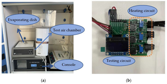
Figure 1.
The laboratory equipment and background. (a) Gas testing laboratory. (b) Homemade electronic nose.
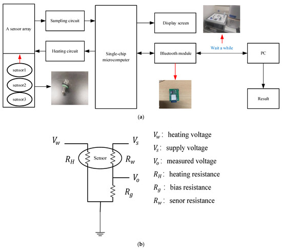
Figure 2.
A schematic diagram of the experiment and measurement circuit. (a) Schematic diagram of the experiment; (b) measurement circuit.
The sensor’s composite material gas sensing probe detects the change in the gas sample concentration and the voltage signal changes caused by the resistance change of the material. The working current of the electronic nose system is 10~80 mA, the output voltage of the test circuit is 0~5 V, and the output voltage of the heating circuit is adjustable (from 5 V to 10 V). The array is placed in a 20-L airbox, and the heating voltage of each gas sensor is adjusted to the optimum operating voltage. The data generated are transmitted to the PC through the Bluetooth module and then controlled by the PC. The entire experimental testing procedure is as follows: (1) The chemical analyte of the required concentration is injected into the gas box, and is evaporated into gas by contacting the evaporating dish; (2) the test gas is kept in the gas box for about 240 s to test the steady-state response of gas; and (3) exhausting the gas for about 300 s to make it easier to test for other types of gas.
As shown in Table 1, the electronic nose system tested three chemical analytes. The measured gases were xylene, acetone, and formaldehyde. For the convenience of expression, the three gases are marked as three separate categories. In this paper, all gases were obtained by evaporating the liquid with different concentrations. Therefore, the concentration is the mass of solute in parts per million of the total solution mass, and ppm is the unit of concentration. The entire experiment lasted for two consecutive months: each test was repeated 60 times, and the number of samples in every category was 300, therefore the measured dataset was 900 in total.

Table 1.
The datasets in detail.
2.2. Methods of Data Sample Prepossessing
In practice, sensors need to be able to work for long hours and such an ideal situation is still impossible to achieve. As a result, it is unavoidable that unpredictable changes will occur such as the drift of sensors and background noises [38]. To improve the interference of external effects on the sensor, the measured voltage of each sensor requires preprocessing. At present, the common data preprocessing methods are the ratio method, the fractional ratio method, etc. Among them, the ratio method is used to remove multiplicative noise and drift, whilst the fractional ratio method is mainly used to remove superimposed noise. Generally, for metal oxide semiconductor gas sensors, the effect of the fractional ratio method is more prominent than the other methods. The fractional ratio method is as follows:
where is the response signal of sensor i to sample k, and is the response signal of sensor i to the reference sample. The time variables were sampled according to the aforementioned measurement process, generating a total of 2000 points. Assuming that the sample vectors of each sensor are S1, S2, and S3, three acquired sample vectors will be integrated into one matrix, which is expressed as S(i) = [S1; S2; S3]. In this paper, the algorithm’s reliability was confirmed with a ten-fold cross-validation method. As a consequence, there were 810 pieces of training data and 90 pieces of test data. Figure 3a shows three typical sensor responses with different gases. Meanwhile, the chemical analytes were xylene (100 ppm), acetone (300 ppm), and formaldehyde (100 ppm). Figure 3b shows the sample with 60 times resampling.
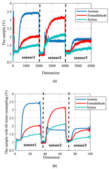
Figure 3.
The original sample and the sample with 60 times resampling. (a) The original sample; (b) The sample with 60 times resampling.
2.3. Pattern Recognition Based on SRC
At present, SRC has been proven to be robust and has a high identification rate in the presence of noise, even when part of the data is missing.
As a result, the algorithm works well in the application of electronic noses. The basic principle of the sparse representation aims to discover a set of bases that is sufficiently sparse and to express the original sample with it. Figure 4 shows the basic principle of SRC. The non-white part represents a non-zero element, and the white part represents that element is zero. Meanwhile, different colors express different values. Therefore, an input signal can be expressed as [39]:
where X is the sparse representation coefficient; Y is an input signal; S is a dictionary. To solve the problem better, Equation (2) can be transformed into:
where is the number of non-zero entries in matrix X. Equation (3) expresses how to minimize the non-zero term of the matrix X and satisfy the conditions . By calculating the reconstruction error between the reconstructed sample and the original sample, it can determine the class label. The reconstruction error can be expressed as [40]:
where E is the reconstruction residual. The reconstruction error can reflect the characteristics of the input signal. It is straightforward from Equation (3) that the sparse representation classification algorithm usually uses the l0-norm or l1-norm minimization approach to process data and accomplishes the pattern recognition job. However, solving the norm minimization issue is an NP-hard task that takes a considerable calculation time. Many researchers have presented various strategies to handle this problem such as gradient projection, proximal gradient, iterative shrinkage threshold, and so on. As a result, overcoming this disadvantage is a critical issue.
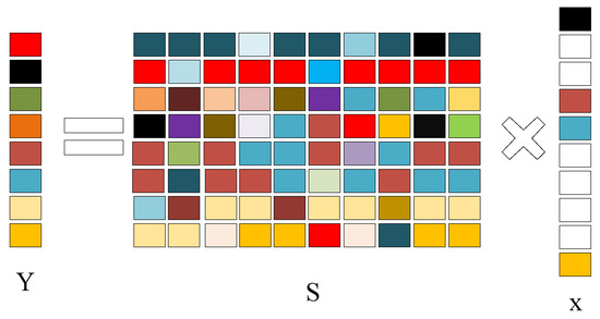
Figure 4.
A schematic diagram of the SRC.
2.4. Pattern Recognition Based on K-SVD
In sparse decomposition models, a suitable dictionary is crucial, and it can have a significant impact on the entire algorithm. Dictionary learning algorithms have received a lot of interest in recent years [41]. Meanwhile, the dictionary learning algorithm is developed from the clustering method. The K-SVD algorithm is an iterative algorithm and it updates the coding coefficients one by one. The concept of K-SVD can be explained by addressing the following model’s minimization problem [42]:
where is the column in dictionary S; is the error caused by atoms other than the atom. It can be seen from Equation (5) that the K-SVD algorithm updates the atoms one by one by analyzing the atom separately. The singular value decomposition (SVD) can update the atoms and coefficients of the dictionary, and it is used to find the matrix with the closest distances, reducing the reconstruction error of the signal. Then, the singular value decomposition is used to apply to [43]. To ensure the accuracy of signal reconstruction and sparse constraints, only the non-zero items are retained, and all other zero items are removed. First, the coordinates of the corresponding elements are defined as . Then, a matrix is constructed and the value of is 1, and the others is 0. Figure 5 mainly summarizes the process of traditional K-SVD algorithms.
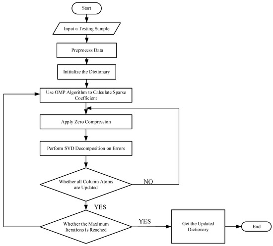
Figure 5.
The flowchart of the traditional K-SVD algorithms.
2.5. Improved Dictionary Learning Algorithm
The traditional K-SVD dictionary learning algorithm updates the dictionary with only a single column of atoms in an iteration, which significantly slows down the process. The goal of this paper was to change the process of updating dictionaries by updating several atoms at the same time, so that unnecessary computations can be avoided. The least-squares approach was employed to tackle the issue, and the sparse matrix was decomposed using SVD to simplify the formula, further reducing the computational burden and improving the algorithm’s learning effectiveness. Dictionary learning classification techniques often need initialization of the dictionary, sparse coding, and dictionary updates as well as classification. First, the dictionary is initialized by a normalized Gaussian random matrix. The number of atomic columns is set to k in the stage of updating the dictionary, and the reconstruction error is:
where can be expressed as ; is the iteration of the sparse matrix from the row to the row , and is the iteration of the dictionary from the column to the column . By applying the least-squares method in Equation (6), it can be expressed as:
By applying the SVD algorithm to decompose W in Equation (7), then it is expressed as follows:
where Q is a diagonal and full-rank matrix. By bringing Equation (8) into Equation (7), it can be expressed as:
where is an orthogonal matrix. According to the Equation (9), it can be expressed as:
2.6. A Proposed Classification Model
In this section, aiming at the problem that the K-SVD dictionary learning algorithm is not discriminative, a new classification algorithm was proposed. Figure 6 shows the basic principle of the new model. During the process of updating the dictionary, all of the training samples are split into i pieces by a simple linear projection. To make the dictionary disclose that the training samples of the category differed from other categories, an assumption was made that the coefficients acquired by projection were concentrated in the sparse matrix of the same categories, and the internal distance of the coefficients was small. The value of coefficients belonging to the training samples of the other categories was extremely low.
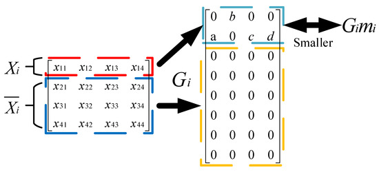
Figure 6.
A schematic diagram of the new model.
As a result, the new model may be represented as follows:
where is a full-rank matrix; and are incoherent; is the transpose of ; is the complementary data matrix of in the whole training sample; and are regularization parameters in order to avoid a high risk of overfitting to training samples; is the mean of the ; is the vector of ; n is the number of .
The formula denotes that the feature of a matrix may be disclosed by a simple linear projection. The formula expresses that the coefficients belonging to the training samples of the other categories are extremely few. The formula expresses that the distance of the coefficients belonging to the same categories’ training samples is small. This concept may be employed to increase the algorithm’s overall discriminative capacity.
By taking the partial derivative to Equation (11) and it can be expressed as:
As a result, the following formula can be obtained:
In this paper, the orthogonal matching pursuit (OMP) was adopted to calculate the sparse coefficients [44]. In order to calculate the reconstructed samples, the application formula was as follows:
By reconstructing the test sample, and calculating the reconstruction errors between the test sample and the reconstructed sample, the classification of different gases can be written as:
Figure 7 summarizes the process of the improved algorithm.
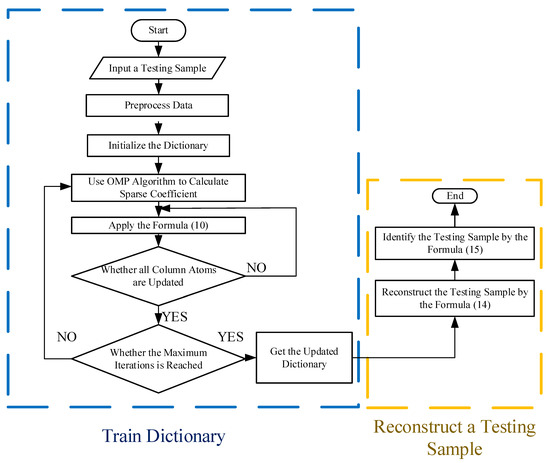
Figure 7.
The flowchart of the improved algorithm.
2.7. The Analysis of Time Complexity
Usually, an algorithm can be assessed by the time complexity or space complexity [45]. This paper only analyzed the time complexity from the part of updating the dictionary. Here, the number of training samples was m, the dimension of datasets was n, the number of atoms was r, and the dimension of the diagonal matrix was h.
First, the traditional K-SVD dictionary learning algorithm was analyzed, where Equation (5) requires about multiplications and subtractions, and the time complexity is O. Then, the singular value decomposition of requires operations, and the time complexity is O. The formula needs operations, and the time complexity is O. Hence, completing the part of updating all atomic columns requires:
Then, the time complexity analysis of the improved algorithm was analyzed. From Equation (6), it can be seen that the formula requires operations, and the time complexity is O. The singular decomposition of a sparse matrix requires operations, and the time complexity is O. The formula requires three multiplications including the process of the inversion. In fact, only the diagonal element of the diagonal matrix Q needs to be calculated because Q is a diagonal matrix, so inverting the matrix Q only requires operations. Among them, the formula requires about operations, and right multiplying matrix requires operations. Finally, right multiplying requires operations. Hence, completing the part of updating all atomic columns requires:
It can be seen from Equations (16) and (17) that it was not easy to observe the magnitude relationship. For simplicity, by calculating the difference between Equation (17) and Equation (16) under the certain case: h = 6; m = 270; n = 24, it can be expressed as:
Figure 8 shows the relationship between the computational complexity and the number of updated atomic columns. When the number of updated atomic columns is larger than 5, the computational complexity increases with the increase in the number of updated atomic columns. When the number of updated atomic columns is larger than 15, the curve increases more slowly with the increase in the number of updated atomic columns. Finally, the theoretical analysis proves that the proposed algorithm reduces the computational complexity to a certain extent.
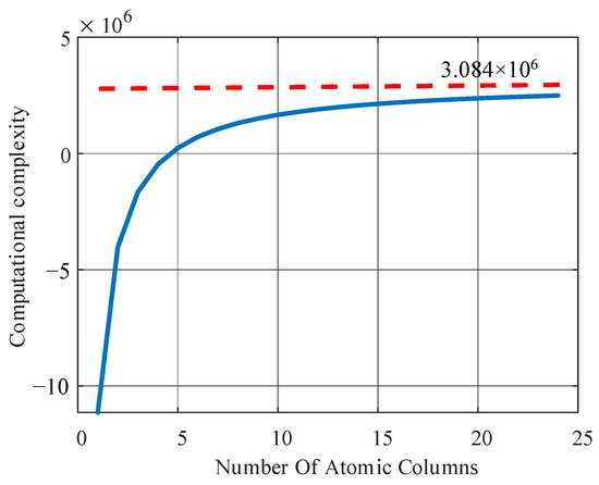
Figure 8.
The relationship between the computational complexity and the number of updated atomic columns.
2.8. The Analysis of Incoherence and Sparsity
Usually, the incoherence and sparsity are critical for reconstruction. These decide whether the algorithm can reconstruct original samples. First, the incoherence of the dictionary is calculated as [46]:
when , and are incoherent. The experimental results showed that when the dimension of the datasets is set to 128, is the maximum. In this case, the maximum coherence between and of ten iterations is shown in Table 2. As a result, it satisfies the incoherence condition.
Table 2.
The coherence between and .
Second, Figure 9 shows that the coding coefficients were obtained by training . As shown in Figure 9, the coefficients of were very small, while a few large coefficients were concentrated in . As a result, it satisfies the sparsity condition.
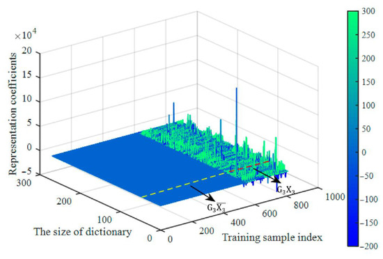
Figure 9.
The coefficient matrix.
As a result, the new model proposed in this paper satisfies two conditions and it can construct the sample successfully.
3. Results and Discussion
3.1. Feasibility Analysis
The experimental results of all algorithms were tested in MATLAB R2018a. This part utilized the ten-fold cross-validation approach to assess the algorithm’s performance and validate the algorithm’s properties in this research. By dividing the datasets into ten parts, nine of them were used as training samples and one was used as the testing samples. In this section, acetone was a testing sample. Figure 10a shows the original sample. Figure 10b–d shows the reconstructed samples of their corresponding categories. By reconstructing the original sample signal, the test sample can be rebuilt. It is clear that the original sample belonged to the second category of samples. Finally, it was easy to determine that the input gas was acetone, demonstrating the viability of the proposed method.
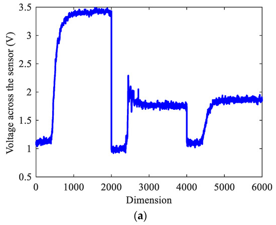
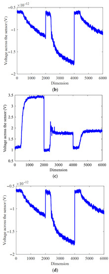
Figure 10.
The testing sample and reconstructed samples. (a) Testing sample. (b) The 1th class reconstructed sample. (c) The 2th class reconstructed sample. (d) The 3th class reconstructed sample.
3.2. Analysis of Parameters
In this section, the dimension of the datasets was set to 18. When and have different values, the recognition accuracy of the proposed algorithm is calculated. As a result, the choice of parameters is particularly important. Figure 11 shows that the different parameters seriously affected the recognition rate.
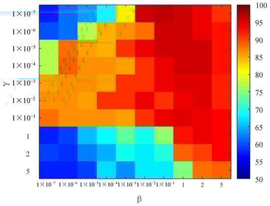
Figure 11.
The recognition accuracy of different and .
When different rule parameters were selected, the recognition rate was very different. When and , the gas recognition accuracy was lower than 80. When 5 and ,the gas recognition accuracy was higher than 80. In this case, when , the gas recognition accuracy was high, which means that the inter-class distance term is more important than . When , the gas recognition accuracy was very low. In other cases, the overall recognition rate was not regular 1 × 10⁻⁷.
To sum up, Figure 11 shows that when and were set to 0.1, the recognition accuracy was the highest.
3.3. Characteristic Analysis of Improved Algorithm
To further evaluate the effectiveness of the proposed algorithm, Figure 12 shows the relationship between the training time of the improved algorithm and the number of updated dictionary columns. The dimension of the datasets was reduced from 6000 dimensions to 24 dimensions by the resampling method. When the number of atomic columns k was smaller than 18, the training time of the algorithm in this paper decreased slowly with the increase in the number of atomic columns and the average training time was larger than 10 s. When the number of atomic columns k was larger than 18, the training time did not continue to decrease, and the average training time was about 7.76 s. The experimental findings suggest that the method presented in this work is the fastest when the number of columns is 18.
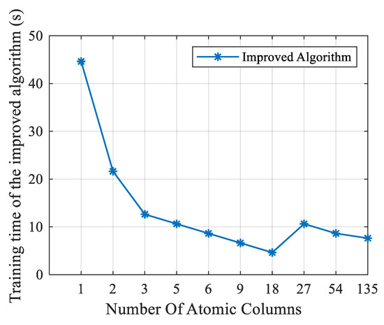
Figure 12.
The relationship between the number of atomic columns and the training time.
3.4. The Comparison of the Improved Method with Other Methods
To demonstrate the advantage of the proposed algorithm in this work, label consistent K-SVD (LC-KSVD) [47], sequential generalization of a k-means (SGK) [48], support vector machine (SVM), and the decision tree algorithm are well-known methods. Therefore, they were built as a comparison in this section. The study in [49] proposed a new classification model for the dictionary learning algorithm and applied it to the K-SVD and SGK. The parameters were set to 0.01. In this paper, these were called the KSVD-DL and SGK-DL. Typically, the dimension impacts the algorithm performance, which affects the training time and the size of the matrix. As a result, the performance of the algorithms with varied dimensions was analyzed in this study. Figure 13 shows the recognition accuracy of different algorithms and the improved algorithm. The best parameters of the improved algorithm changed with the increase in the dimension. Therefore, for different dimensions, the parameters were set to different values. The average accuracy of SVM was nearly 82.57%. The average accuracy of SVM was significantly worse than the improved algorithm, decision tree, and KSVD-DL algorithm. The average accuracy of the decision tree was nearly 87.99%. When the dimension of the sample was smaller than 10, the decision tree outperformed the improved algorithm and KSVD-DL algorithm. When the dimension of the sample was larger than 10, the average accuracy of the improved algorithm was greater than the other traditional algorithms and increased with the increase in dimension. Figure 14 and Table 3 show the comparison results between the different algorithms and the improved algorithm. The number of atomic columns of the improved algorithm was 18, and the average training time of the proposed algorithm was faster than the KSVD-DL algorithm by about 7.33 s and the SGK-DL algorithm by about 21.41 s.
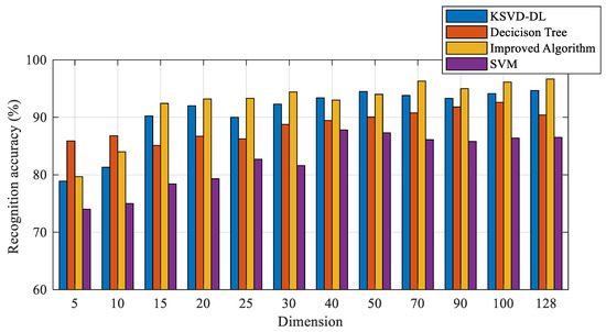
Figure 13.
The recognition accuracy of the traditional algorithm and improved algorithm.
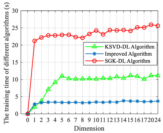
Figure 14.
The training time of the traditional algorithm and improved algorithm.
Table 3.
The comparison of the improved method with other methods (sample dimension M = 24).
To prove the advantage of the improved algorithm, we performed the Nemenyi test to show the difference between the improved algorithm and other algorithms. p is the standard for significant difference [50]. When p < 0.05, both different algorithms are significantly different. Table 4 shows that our algorithm was significantly different from the SVM and decision tree. Although it is not significantly different from KSVD-DL, the proposed algorithm has certain advantages in other aspects such as the low average training time. When the dimension of the sample is larger than 10, the average recognition accuracy of the improved algorithm is maintained above 90%, and the average training time of the algorithm is controlled within 4 s. The proposed algorithm achieved the highest average recognition accuracy among all algorithms included in the comparison. The experimental results showed that the algorithm proposed in this paper is a more effective method for an electronic nose than the traditional dictionary learning algorithms.
Table 4.
The experimental results of the Nemenyi test.
For further comparison with other dictionary algorithms, the reconstruction residual error can be considered as the standard of the classification precision in this section. As shown in Figure 15a,b, it can be found that the 1st reconstruction residual was smaller than the KSVD-DL by about 110. Since the proposed model imposes a constraint that the coefficients in the same category should keep a large coefficient and be closer to their class centers, it allows for the reconstruction of the same category to be more precise. The result demonstrates that the improved method had a better classification precision.
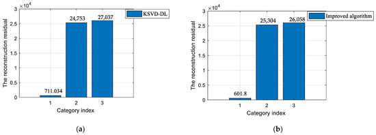
Figure 15.
The comparison results between the improved method and other methods. (a) The residual of the KSVD-DL algorithm. (b) The residual of the improved algorithm.
In summary, the proposed algorithm can achieve a competitive recognition accuracy for gas classification. Meanwhile, it greatly reduces the running time of the algorithm.
4. Conclusions and Outlook
In this article, a novel dictionary learning method was proposed for gas classification. The comparison results between the improved algorithm and different classification algorithms demonstrated that the proposed algorithm could achieve a high recognition accuracy and a relatively lower running time. In the training phase, the algorithm performed a multi-column atomic update, which reduced the running time better than the traditional single-column atomic methods. Meanwhile, in the testing phase, a novel classification model was proposed to effectively increase the discriminative power and the average recognition accuracy of the whole algorithm. When the dimension of the sample was larger than 10, the average recognition rate of the algorithm was maintained above 92%, and the average training time was controlled within 4 s. As a result, it is a feasible means to detect VOC gases in the environmental industry, chemical industry, and petroleum industry.
However, there are still many problems associated with its practical application. First, electronic noses are extremely sensitive to the environment, which results in issues such as the inability to collect reliable data. Furthermore, most sensors can induce aging over time. Therefore, the algorithm must be predictive. Another difficult challenge is how to obtain a good sample for practical applications. These problems have a significant impact on the evolution of electronic noses and will be an important direction for future work. With the rising number of researchers in the fields of materials science and data analysis, gas recognition based on e-nose technology might soon reach new heights.
Author Contributions
Conceptualization, S.S.; Methodology, J.H. and H.J.; Software and hardware, H.J. and C.G.; Writing—original draft preparation, H.J. and C.G.; Writing—review and editing, J.H. and H.J.; Supervision, J.H. and S.S. All authors have read and agreed to the published version of the manuscript.
Funding
This research received no external funding.
Data Availability Statement
Not applicable.
Conflicts of Interest
The authors declare no conflict of interest.
References
- Ekmekçioğlu, A.; Ünlügençoğlu, K.; Çelebi, U.B. Container ship emission estimation model for the concept of green port in Turkey. Proc. Inst. Mech. Eng. Part M: J. Eng. Marit. Environ. 2022, 236, 504–518. [Google Scholar] [CrossRef]
- Taştan, M.; Gökozan, H. Real-Time Monitoring of Indoor Air Quality with Internet of Things-Based E-Nose. Appl. Sci. 2019, 9, 3435. [Google Scholar] [CrossRef]
- Basu, M.; Bunke, H.; Del Bimbo, A. Guest editors’ introduction to the special section on syntactic and structural pattern recognition. IEEE Trans. Pattern Anal. Mach. Intell. 2005, 27, 1009–1012. [Google Scholar] [CrossRef] [PubMed]
- Ho, T.K.; Baird, H.S. Large-scale simulation studies in image pattern recognition. IEEE Trans. Pattern Anal. Mach. Intell. 1997, 19, 1067–1079. [Google Scholar] [CrossRef]
- Keysers, D.; Macherey, W.; Ney, H.; Dahmen, J. Adaptation in statistical pattern recognition using tangent vectors. IEEE Trans. Pattern Anal. Mach. Intell. 2004, 26, 269–274. [Google Scholar] [CrossRef]
- Yue, Y.; Yang, T.; Zeng, X. Seismic denoising with CEEMD and KSVD dictionary combined training. Oil Geophys. Prospect. 2019, 54, 729–736. [Google Scholar] [CrossRef]
- Zhang, S.; Xia, X.; Xie, C.; Cai, S.; Li, H.; Zeng, D. A method of feature extraction on recovery curves for fast recognition application with metal oxide gas sensor array. IEEE Sens. J. 2009, 9, 1705–1710. [Google Scholar] [CrossRef]
- Di Natale, C.; Macagnano, A.; Martinelli, E.; Falconi, C.; Galassi, E.; Paolesse, R.; D’Amico, A. Application of an Electronic Nose to the Monitoring of a Bio-technological Process for Contaminated Limes Clean. In Electronic Noses and Olfaction 2000, Proceedings of the 7th International Symposium on Olfaction and Electronic Noses, Brighton, UK, 10 July 2000; CRC Press: Brighton, UK, 2001. [Google Scholar]
- Bezdek, J.C. Pattern Recognition with Fuzzy Objective Function Algorithms; Plenum Press: New York, NY, USA, 1981. [Google Scholar] [CrossRef]
- Ozinsky, A.; Underhill, D.M.; Fontenot, J.D.; Hajjar, A.M.; Smith, K.D.; Wilson, C.B.; Aderem, A. The repertoire for pattern recognition of pathogens by the innate immune system is defined by cooperation between toll-like receptors. Proc. Natl. Acad. Sci. 2000, 97, 13766–13771. [Google Scholar] [CrossRef] [PubMed]
- Pardo, M.; Sberveglieri, G. Classification of electronic nose data with support vector machines. Sens. Actuators B Chem. 2005, 107, 730–737. [Google Scholar] [CrossRef]
- Hierlemann, A.; Weimar, U.; Kraus, G.; Schweizer-Berberich, M.; Göpel, W. Polymer-based sensor arrays and multicomponent analysis for the detection of hazardous oragnic vapours in the environment. Sens. Actuators B Chem. 1995, 26, 126–134. [Google Scholar] [CrossRef]
- He, X.; Yan, S.; Hu, Y.; Niyogi, P.; Zhang, H.J. Face recognition using laplacianfaces. IEEE Trans. Pattern Anal. Mach. Intell. 2005, 27, 328–340. [Google Scholar] [CrossRef]
- Weng, X.; Kong, C.; Jin, H.; Chen, D.; Li, C.; Li, Y.; Ren, L.; Xiao, Y.; Chang, Z. Detection of Volatile Organic Compounds (VOCs) in Livestock Houses Based on Electronic Nose. Appl. Sci. 2021, 11, 2337. [Google Scholar] [CrossRef]
- Han, X.; Lü, E.; Lu, H.; Zeng, F.; Qiu, G.; Yu, Q.; Zhang, M. Detection of Spray-Dried Porcine Plasma (SDPP) based on Electronic Nose and Near-Infrared Spectroscopy Data. Appl. Sci. 2020, 10, 2967. [Google Scholar] [CrossRef]
- Edelman, B.; VALEntin, D.; Abdi, H. Sex classification of face areas: How well can a linear neural network predict human performance? J. Biol. Syst. 2011, 6, 241–263. [Google Scholar] [CrossRef]
- Boiman, O.; Shechtman, E.; Irani, M. In defense of nearest-neighbor based image classification. In Proceedings of the 2008 IEEE Conference on Computer Vision and Pattern Recognition, Anchorage, AK, USA, 23–28 June 2008. [Google Scholar] [CrossRef]
- Chapelle, O.; Haffner, P. SVMs for Histogram-Based Image Classification. IEEE Trans. Neural Netw. 1999, 10, 1055–1064. [Google Scholar] [CrossRef] [PubMed]
- Li, K.; He, F.; Chen, X. Real-time object tracking via compressive feature selection. Front. Comput. Sci. 2016, 10, 689–701. [Google Scholar] [CrossRef]
- Yang, X.; Wang, M.; Zhang, L.; Sun, F.; Hong, R.; Qi, M. An efficient tracking system by orthogonalized templates. IEEE Trans. Ind. Electron. 2016, 63, 3187–3197. [Google Scholar] [CrossRef]
- Jin, C.; Park, S.; Kim, H.; Lee, C. Enhanced H2S gas-sensing properties of Pt-functionalized In2Ge2O7 nanowires. Appl. Phys. A 2014, 114, 591–595. [Google Scholar] [CrossRef]
- Guo, D.; Zhang, D.; Zhang, L. Sparse representation-based classification for breath sample identification. Sens. Actuators B Chem. 2011, 158, 43–53. [Google Scholar] [CrossRef]
- Xu, Y.; Zhang, Z.; Lu, G.; Yang, J. Approximately symmetrical face images for image preprocessing in face recognition and sparse representation based classification. Pattern Recognit. 2016, 54, 68–82. [Google Scholar] [CrossRef]
- Gao, Y.; Liao, S.; Shen, D. Prostate segmentation by sparse representation based classification. Med. Phys. 2012, 39, 6372–6387. [Google Scholar] [CrossRef] [PubMed][Green Version]
- Min, R.; Dugelay, J.L. Improved combination of LBP and sparse representation based classification (SRC) for face recognition. In Proceedings of the 2011 IEEE International Conference on Multimedia and Expo, Barcelona, Spain, 11–15 July 2011. [Google Scholar] [CrossRef]
- Schnass, K. On the identifiability of overcomplete dictionaries via the minimisation principle underlying K-SVD. Appl. Comput. Harmon. Anal. 2014, 37, 464–491. [Google Scholar] [CrossRef][Green Version]
- Jiang, Z.; Lin, Z.; Davis, L.S. Label consistent K-SVD: Learning a discriminative dictionary for recognition. IEEE Trans. Pattern Anal. Mach. Intell. 2013, 35, 2651–2664. [Google Scholar] [CrossRef] [PubMed]
- Yu, F.; Xi, J.; Zhao, L.; Zou, C. Sparse presentation of underdetermined blind source separation based on compressed sensing and K-SVD. Journal of Southeast University. Nat. Sci. Ed. 2011, 41, 1127–1131. [Google Scholar] [CrossRef]
- Zhai, X.; Zhu, W.; Kang, B. Compressed sensing of images combining KSVD and classified sparse representation. Comput. Eng. Appl. 2015, 51, 193–198. [Google Scholar]
- Vila, J.P.; Schniter, P. Expectation-maximization Gaussian-mixture approximate message passing. IEEE Trans. Signal Process. 2013, 61, 4658–4672. [Google Scholar] [CrossRef]
- Bellili, F.; Sohrabi, F.; Yu, W. Generalized approximate message passing for massive MIMO mmWave channel estimation with Laplacian prior. IEEE Trans. Commun. 2019, 67, 3205–3219. [Google Scholar] [CrossRef]
- Zhu, T. New over-relaxed monotone fast iterative shrinkage-thresholding algorithm for linear inverse problems. IET Image Process. 2019, 13, 2888–2896. [Google Scholar] [CrossRef]
- Khoramian, S. An iterative thresholding algorithm for linear inverse problems with multi- constraints and its applications. Appl. Comput. Harmon. Anal. 2012, 32, 109–130. [Google Scholar] [CrossRef]
- Chang, X.; Xu, S.; Liu, S.; Wang, N.; Zhu, Y. Highly sensitive acetone sensor based on wo3 nanosheets derived from ws2 nanoparticles with inorganic fullerene-like structures. Sens. Actuat. B Chem. 2021, 343, 130135. [Google Scholar] [CrossRef]
- Sun, S.; Wang, M.; Chang, X.; Jiang, Y.; Zhang, D.; Wang, D.; Zhang, Y.; Lei, Y. W18O49/Ti3C2Tx Mxene nanocomposites for highly sensitive acetone gas sensor with low detection limit. Sens. Actuat. B Chem. 2020, 304, 127274. [Google Scholar] [CrossRef]
- Zhu, X.; Zhang, X.; Chang, X.; Li, J.; Pan, L.; Jiang, Y.; Sun, S. Metal-organic framework-derived porous SnO2 nanosheets with grain sizes comparable to Debye length for formaldehyde detection with high response and low detection limit. Sens. Actuat. B Chem. 2021, 347, 130599. [Google Scholar] [CrossRef]
- Sun, S.; Xiong, X.; Han, J.; Chang, X.; Wang, N.; Wang, M.; Zhu, Y. 2D/2D Graphene Nanoplatelet–Tungsten Trioxide Hydrate Nanocomposites for Sensing Acetone. ACS Appl. Nano Mater. 2019, 2, 1313–1324. [Google Scholar] [CrossRef]
- Sajan, R.I.; Christopher, V.B.; Kavitha, M.J.; Akhila, T.S. An energy aware secure three-level weighted trust evaluation and grey wolf optimization based routing in wireless ad hoc sensor network. Wirel. Netw. 2022, 28, 1439–1455. [Google Scholar] [CrossRef]
- Yin, J.; Liu, Z.; Zhong, J.; Yang, W. Kernel sparse representation based classification. Neurocomputing 2012, 77, 120–128. [Google Scholar] [CrossRef]
- Qu, S.; Liu, X.; Liang, S. Multi-Scale Superpixels Dimension Reduction Hyperspectral Image Classification Algorithm Based on Low Rank Sparse Representation Joint Hierarchical Recursive Filtering. Sensors 2021, 21, 3846. [Google Scholar] [CrossRef]
- Yuan, X.T.; Liu, X.; Yan, S. Visual classification with multitask joint sparse representation. IEEE Trans. Image Process. 2012, 21, 4349–4360. [Google Scholar] [CrossRef]
- Aharon, M.; Elad, M.; Bruckstein, A. K-SVD: An algorithm for designing overcomplete dictionaries for sparse representation. IEEE Trans. Signal Process. 2006, 54, 4311–4322. [Google Scholar] [CrossRef]
- Zermi, N.; Khaldi, A.; Kafi, M.R.; Kahlessenane, F.; Euschi, S. Robust SVD-based schemes for medical image watermarking. Microprocess. Microsy 2021, 84, 104134. [Google Scholar] [CrossRef]
- Bruckstein, A.M.; Donoho, D.L.; Elad, M. From sparse solutions of systems of equations to sparse modeling of signals and images. SIAM Rev. 2009, 51, 34–81. [Google Scholar] [CrossRef]
- Zhang, R.Y.; Lavaei, J. Sparse semidefinite programs with guaranteed near-linear time complexity via dualized clique tree conversion. Math. Program. 2021, 188, 351–393. [Google Scholar] [CrossRef]
- Baraniuk, R.G. Compressive Sensing [Lecture Notes]. IEEE Signal. Process. Mag. 2007, 24, 118–121. [Google Scholar] [CrossRef]
- Gu, X.; Zhang, C.; Ni, T. A Hierarchical Discriminative Sparse Representation Classifier for EEG Signal Detection. IEEE/ACM Trans. Comput. Biol. Bioinform. 2021, 18, 1679–1687. [Google Scholar] [CrossRef]
- Sahoo, S.K.; Makur, A. Replacing K-SVD with SGK: Dictionary training for sparse representation of images. In Proceedings of the 2015 IEEE International Conference on Digital Signal Processing (DSP), Singapore, 21–24 July 2015; pp. 614–617. [Google Scholar] [CrossRef]
- He, A.; Wei, G.; Yu, J.; Tang, Z.; Lin, Z.; Wang, P. A novel dictionary learning method for gas identification with a gas sensor array. IEEE Trans. Indust. Electron. 2017, 64, 9709–9715. [Google Scholar] [CrossRef]
- Liu, Y.; Wang, L.; Mammadov, M. Learning semi-lazy Bayesian network classifier under the c.i.i.d assumption. Knowl.-Based Syst. 2020, 208, 422. [Google Scholar] [CrossRef]


Publisher’s Note: MDPI stays neutral with regard to jurisdictional claims in published maps and institutional affiliations. |
© 2022 by the authors. Licensee MDPI, Basel, Switzerland. This article is an open access article distributed under the terms and conditions of the Creative Commons Attribution (CC BY) license (https://creativecommons.org/licenses/by/4.0/).