The Wheel Flat Identification Based on Variational Modal Decomposition—Envelope Spectrum Method of the Axlebox Acceleration

Abstract

The wheel flat can cause train and rail system infrastructure damage and endanger the running safety. To monitor the early wheel flat, it is urgent to carry out the theoretical basic research on the relationship between the vibration signal and the wheel flat. Moreover, to extract the characteristics of the wheel flat, an advanced and effective signal processing method need to be studied. A three-dimensional vehicle-track coupled dynamics model verified by field test is established based on the multi-body dynamics at first. The acceleration of the axlebox excited by the different wheel flat length is obtained by the dynamic simulation. The simulation considers the influence of various speeds and the short-wavelength track irregularities. Then, a combined method based on the variational modal decomposition (VMD) and the envelope spectrum (ES) is employed to detect the wheel flat signal. The feasibility of the method is further validated by comparing the co-existence of the wheel flat and the wheel eccentricity. Finally, field test is carried out to detect the wheel flat by using this method. The results indicate that the VMD-ES method accurately extracts the impact characteristics of the wheel flat and can quantitatively identify the wheel flat faults of small sizes.

1. Introduction

The wheel flat is a common damage caused by emergency braking or wheel sliding during the running process, which has great influence on the running stability and safety. The flat wheel can generate considerable wheel-rail impact. It produces great stress action near the gearbox housing, resulting in housing cracks [1,2], as well as producing a significant impact on the brake disc [3]. Moreover, the high-frequency vibration generated by the wheel flat can act on the rail and sleeper, and then shorten their service life [4]. The damage caused by the wheel flat is even more serious, along with the speed of vehicle and axle loads, which are higher than ever before. Therefore, it is necessary to adopt an efficient signal processing method for the early wheel flat detection.

Nowadays, scheduled repair and periodic flaw detection are used to identify and deal with the wheel damage at workshops. To ensure the running safety, formulating a short maintenance cycle is inevitable, which increases the maintenance costs and unnecessary downtime. Hence, monitoring and tracking the wheel flat in real-time with signal processing methods can greatly enhance the economic efficiency. It is necessary to monitor the wheel status in real-time and use a linear index to quantitatively evaluate the flat faults. The transformation of the wheel maintenance from planned repair to state repair is the inevitable trend in the future.

The wheel flat identification attracted considerable attention decades ago, and the related researches have been gradually increasing in the last decade [5]. The establishment of an efficient method to identify the wheel flat is still the subject of many researches at present. The wheel flat identification method are mainly divided into two groups: the wayside method and the on-board method.

The wayside method monitors the wheel status with a series of sensors mounted on the rail. Mosleh et al. [6] adopted the envelope spectrum to detect the wheel flat signal based on the shear force of the rail. Alireza et al. [7] fused the data measured by multiple stress sensors and correlated it with the circumferential position of the wheel. Cao et al. [8] proposed a two-step important point selection method based on the time series with the multilayered sensing device. Besides the aforementioned methods, other types of technology, such as ultrasonic [9,10,11] and fiber optic sensing technology [12,13,14,15], are also reported in the researches of wheel flat identification. However, wayside detection can only detect the wheel flat in a fixed section, and the partial wheel conditions information provided by limited number of sensors reduces the overall reliability of the wheel flat identification [16].

The on-board method monitors the wheel status in real-time by placing the sensors on the vehicle components. The closer the sensor is to the wheelset, the more vibration information of the wheel is reflected. To extract the vibration characteristics of the wheel, more accurate signal analysis methods are needed when the sensor is far away from the wheelset. Liang et al. [17] used the adaptive noise canceling to process the axlebox acceleration signal with flat and compared it with other time-frequency analysis methods. Bosso et al. [18] proposed a time domain index to identify the wheel flat faults, and validated its feasibility by field test on the freight vehicle. Shim et al. [19] transformed the vibration signals from time domain to rotating angular domain with a combined method based on the cepstrum analysis and the order analysis. Shi et al. [20] designed a one-dimensional convolutional neural network. Bernal et al. [21] recorded the bearing adapter acceleration signals on a 1:4 scale bogie test rig, and validated the feasibility of wheel flat analogue fault detector device. The on-board method is lower-cost and the sensor installed on the vehicle is easily maintained. In this work, we will focus on the on-board method to detect the wheel flat. Although the on-board monitoring method was adopted in the above study, the quantitative correspondence between the expansion of the flat and the index still needs further study.

The axlebox is in direct contact with the wheelset, and the characteristics of high frequency vibration between wheel and rail are reflected in it. Meanwhile, the axlebox acceleration is always influenced by the complex wheel-rail excitation (e.g., the track irregularities, wheel polygon and wheel flat). The impact characteristics of the wheel flat are easily covered by interference signal especially in the early wheel flat faults. The accuracy extraction of the wheel flat characteristics makes it a challenge for the wheel flat identification by using the axlebox acceleration. Therefore, the advanced signal processing methods need to be employed to process the fault signal. As an adaptive signal decomposition method, empirical mode decomposition (EMD) [22] was adopted in the wheel flat identification [23,24]. However, its end effect and mode mixing in signal decomposition limits the widely application [25]. As the alternative of EMD, variational mode decomposition (VMD) was proposed by Dragomiretskiy [26], which effectively makes up for the shortcomings of EMD. VMD has been widely employed to diagnose the train axlebox bearing faults [27,28,29], but its effectiveness in the wheel flat identification has not been deeply studied. Similarly, envelope spectrum (ES) is widely applied in the rotating machinery fault diagnosis, which is sensitive to the impact. It is reported that the ES has the potential to identify wheel faults [30]. On the basis of the above discussion, a VMD-ES combined method was proposed to detect the wheel flat faults by using the axlebox acceleration in this paper. The method can eliminate the end effect and mode mixing in signal decomposition, and extract the fault characteristic frequency more efficiently than the original signal spectrum domain.

The structure of this paper is as follows: Section 2 established a three-dimensional vehicle-track coupled dynamics verified by field test to simulate the axlebox acceleration excited by the wheel flat. The VMD-ES method was presented in Section 3. The results of the wheel flat identification based on the method was investigated in Section 4, and the feasibility of the method was further validated by comparing the co-existence of the wheel flat and the wheel eccentricity in Section 5. Then the method validation is carried out with using the data measured from the field test in Section 6. Finally, some conclusions are given in Section 7.

2. Dynamics Model

2.1. Vehicle-Track Coupled Dynamics Model

To simulate the dynamic response of the axlebox acceleration excited by the wheel flat, consider as an example a CRH380B high-speed vehicle, where a three-dimensional vehicle-track coupled dynamics model is established based on the multi-body dynamics [31], as shown in Figure 1. The vertical wheel-rail contact forces are calculated by Kik-Poitrowski model, creep, and tangential force in the contact area are calculated by Kalker’s linearized theory. The differential equation of the vehicle system vibration response is [31]:

$$M\ddot{x}+C\dot{x}+Kx=F$$

(1)

where M, C, and K are the mass, damping, and stiffness matrices, respectively; x is the vehicle displacement; F is the vector of the nonlinear wheel-rail contact forces, which is a function of the track irregularities and the vibration state of the track structure.

The vehicle model consists of one car body, two bogies, eight axleboxes, and four wheelsets. In the model, the dampers, air spring, anti-rolling torsion bar, and traction rod are all expressed by elastic force element. Rails are considered as Timoshenko beams, and fasteners are simulated by special force.

Table 1. Parameters of vehicle dynamic model.

Component	Parameter	Value
Wheelset	Mass (kg)	1627
	Moments of pitch inertia (kg m2)	825
	Moments of roll inertia (kg m2)	132
	Moments of yaw inertia (kg m2)	830
	Nominal rolling radius (m)	0.46
	Wheel tread	S1002G
Axlebox	Mass (kg)	66.7
	Moments of pitch inertia (kg m2)	0.3
	Moments of roll inertia (kg m2)	2
	Moments of yaw inertia (kg m2)	2
Bogie	Mass (kg)	2056
	Moments of pitch inertia (kg m2)	1390
	Moments of roll inertia (kg m2)	2590
	Moments of yaw inertia (kg m2)	3800

lists partial parameters of the vehicle dynamic model.

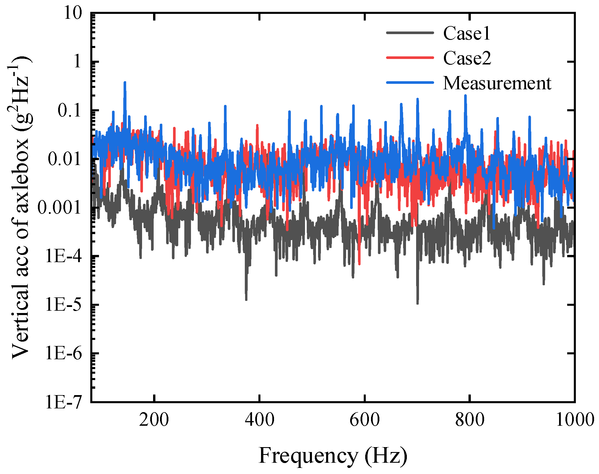
2.2. Model Validation

The axlebox is in direct contact with the wheelset, and the characteristics of high frequency vibration between wheel and rail are reflected in it. The axlebox acceleration of a high-speed EMU was measured from field test at 155.9 km/h. The validation of the vehicle model established in Section 2.1 is verified by comparing the simulated axlebox acceleration with the measurement. Case 1 adopts the ballastless track spectrum of the China high-speed railway. Case 2 includes the track spectrum in Case 1, and the short-wavelength track irregularities in which the wave length range is 0.01–1 m. The comparison between the simulated and measured data is shown in Figure 2.

Figure 2 shows that the amplitude of the axlebox acceleration is small in Case 1, which is far different from the measurement. This is because the track irregularities in Case 1 is the long wave in the range of 1–120 mm, which cannot effectively reflect the actual operating condition. In Case 2, the simulated axlebox acceleration is in good agreement with the measurement, the high frequency excitation caused by the short—wavelength irregularities is directly transmitted from the wheelset to the axlebox. However, due to the track, irregularities cannot completely replace the real line operating conditions and the fastener is simplified into linear force elements, therefore, there are still some differences between the simulated and measured data. It is worth noting that the measured data has the multiple frequency peak with the equal space of 30 Hz, which is caused by 2nd—order wheel polygon ($f_0=nv/(2\pi R)=2\times 155.9/3.6/(2\pi \times 0.46)=30$). Therefore, the track irregularities in Case 2 is used in the simulation. The simulation result is in agreement with the measurement. This ensures the accuracy of the established vehicle model.

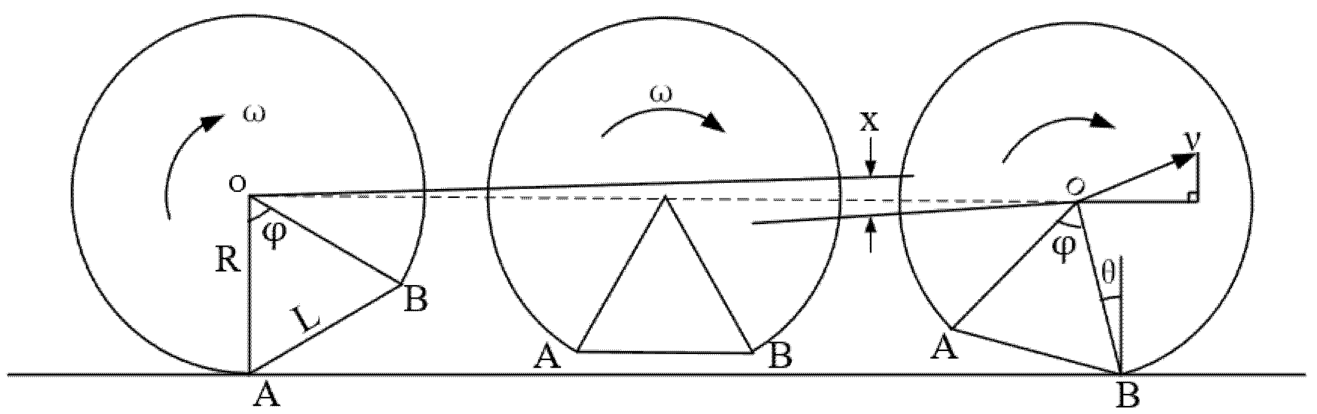
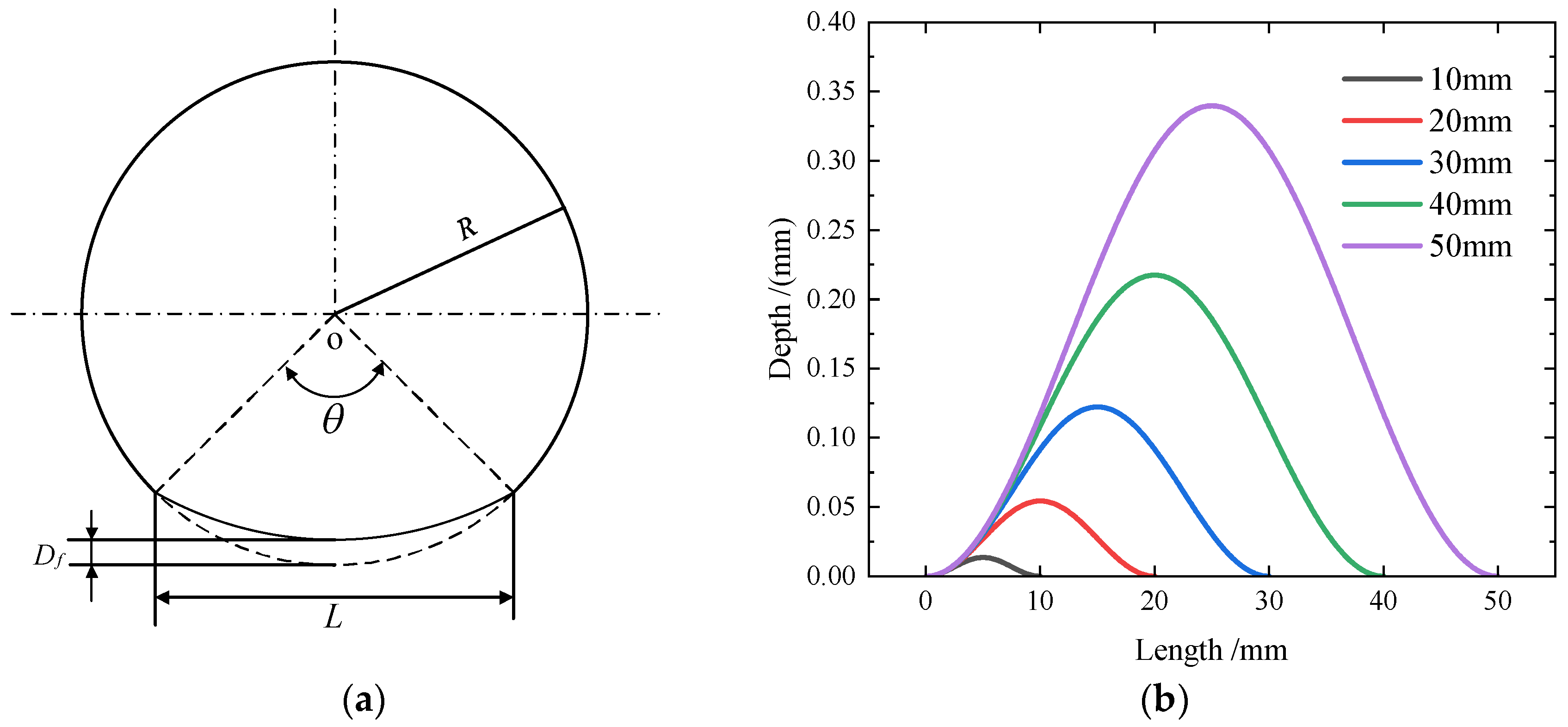
2.3. Wheel Flat Model

When braking or sliding, the wheel can easily appear as local scratch and spalling during train operation resulting in a wheel flat. The wheel flat produces periodic impact which harms the vehicle security. Figure 3 is the motion of the flat wheel when the vehicle is at high speed.

When the vehicle runs at high speed, the wheel rolls to point A at first, then suspends and falls down under the action of inertia. Finally, it contacts the rail surface at point B and produces impact. For high–speed vehicles, the impact velocity of the wheel flat consists of two parts: the speed of the wheel falling from air to track and the vertical component of the wheel center velocity caused by rotation. The wheel impact speed at high speed can be expressed as [31]:

$$v_o=\frac{L}{v+\sqrt{\mu R}}\left(\mu +\gamma v\sqrt{\frac{\mu }{R}}\right)$$

(2)

where L is the length of flat, R is the wheel radius, ν is the speed, γ is the coefficient of wheel rotation inertia transformation into reciprocating inertia, and µ is the wheel acceleration when falling down, which can be expressed as:

$$\mu =\left(M_1+M_2\right)/\left(M_{2}g\right)$$

(3)

where M₁, M₂, are the sprung mass and unsprung mass of the primary suspension, respectively, and g is the gravitational acceleration.

As can be seen from Equation (2), the wheel flat impact velocity is proportional to the length of flat. However, it decreases slightly with the increase of the train speed, and finally approaches a constant value:

$$\overline{v_o}=\underset{v\to \infty }{\lim }{v}_0=\gamma L\sqrt{\frac{\mu }{R}}$$

(4)

The new wheel flat is similar to the chord of a wheel circle. However, when a new flat appears, its edge is quickly worn during the operation, eventually obtaining a rounded one. The field test shows that all the wheel flats of the repaired vehicles are rounded. Therefore, the establishment of a mathematical model with the worn wheel flat to simulate and analyze the impact of wheel flat is necessary. The cosine function is commonly used to describe irregularities in the worn wheel flat [32], which can be expressed as:

$$Z\left(x\right)=\frac{1}{2}{D}_f\left[1-\cos \left(\frac{2\pi x}{L}\right)\right]$$

(5)

where D_f and L are the depth and length of the wheel flat, respectively, x is the running distance, and D_f can be expressed as:

$$D_f=\frac{L^2}{16R}$$

(6)

Figure 4 illustrates the wheel flat model and the relationship between the depth and length of the wheel flat.

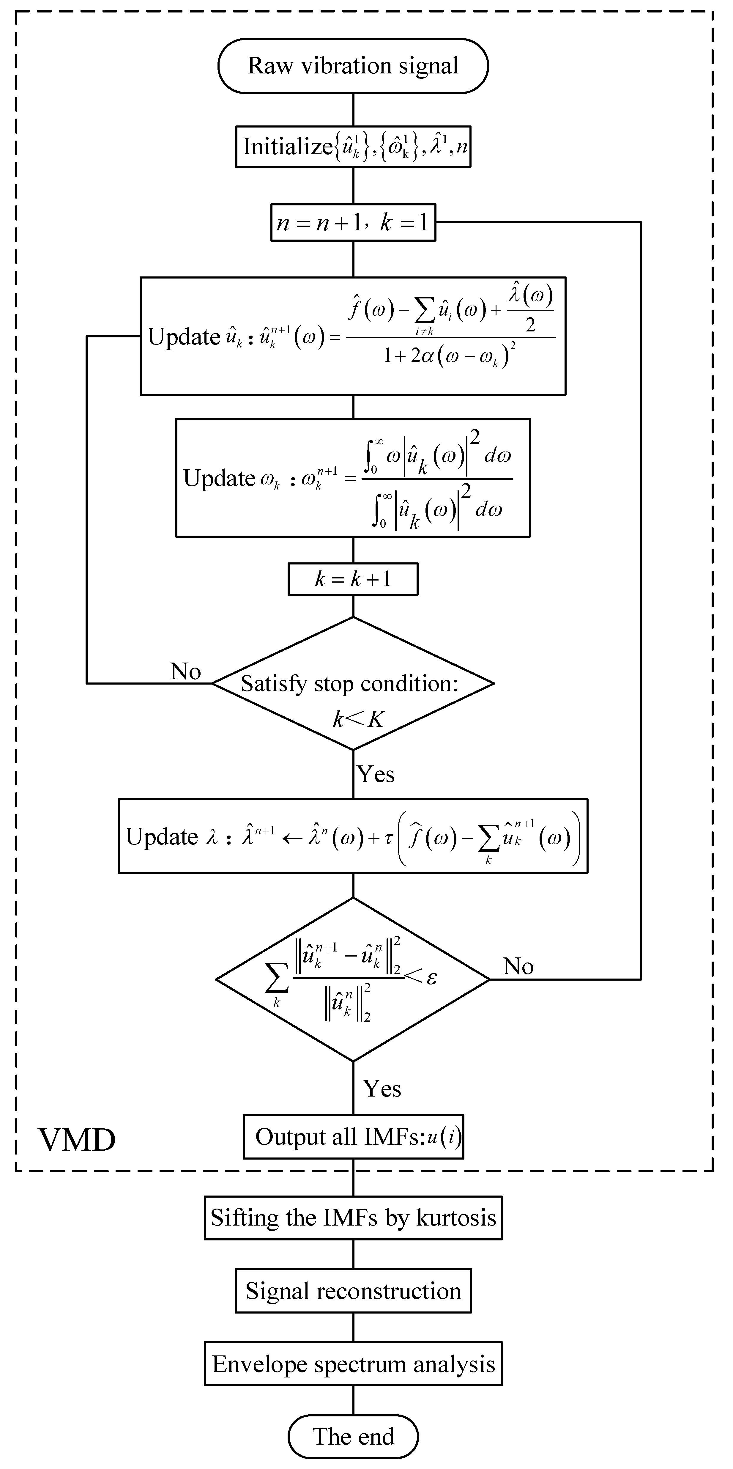
3. Signal Processing Method Based on VMD and ES

Variational modal decomposition (VMD) is an adaptive decomposition method based on Hilbert–Huang transformation, which decomposes the raw signal into a number of intrinsic mode functions (IMFs) by searching the optimal solution of a constrained variational model. The envelope spectrum (ES) is sensitive to the impact, and it can eliminate the interference components and highlight the fault characteristic frequency. Therefore, the VMD-ES method has good adaptability in dealing with the periodic impact generated by the wheel flat.

Figure 5 shows the flow chart of the VMD-ES method. Firstly, the raw signal is decomposed by VMD into a number of IMFs. VMD needs to set number of modal components K and the penalty factor α in advance. In this paper, the decomposition level obtained by EMD is taken as the value of K, and α takes the default value of 2000.

Next, use kurtosis principle [33] to sift the decomposed IMFs and reconstruct the signal. The kurtosis principle is as follows:

$$k=\frac{E{\left(x-\mu \right)}^4}{{\sigma }^4}$$

(7)

where µ is the mean of x, σ is the standard deviation of x, and E(t) represents the expected value of the quantity t.

Third, the reconstructed signal is analyzed by ES as follows:

(1)

Hilbert–Huang transformation is performed on the signal:

$$H\left[x\left(t\right)\right]=\frac{1}{\pi }{\displaystyle {\int }_{-\infty }^{+\infty }\frac{x\left(\tau \right)}{t-\tau }}d\tau$$

(8)

(2)

Obtain envelope spectrum of the signal:

$$B\left(t\right)=\sqrt{x\left(t\right)+H^2\left[x\left(t\right)\right]}$$

(9)

4. Wheel Flat Identification Based on Acceleration of Axlebox

4.1. VMD and IMFs Sifting

The simulated axlebox acceleration is analyzed by the VMD-ES method. This section only lists the process of the VMD and IMFs sifting with the length of 20 mm wheel flat at 350 km/h. Figure 6 shows the result of VMD. According to the principle mentioned in Section 3, the value of number of modal components K is 10.

Figure 6 shows that there is almost no impact components in IMF1 and IMF2. Meanwhile, the impact position and frequency Δf are consistent in IMF3-IMF10, which are generated by the wheel flat. Therefore, VMD can be used to decompose the axlebox acceleration to extract the impact characteristics of the wheel flat from the signals with interference. Then, sift IMFs with the kurtosis principle mentioned in Section 3. The results are shown in

Table 2. Kurtosis value of IMFs.

Components	IMF1	IMF2	IMF3	IMF4	IMF5	IMF6	IMF7	IMF8	IMF9	IMF10
Kurtosis	2.82	2.99	7.39	8.54	11.67	11.74	13.61	12.76	14.93	15.18

.

Kurtosis is a measurement of the outlier tendency in a distribution, which is sensitive to shocks. Table 2 shows that the kurtosis value of IMF1 and IMF2 is much lower than that of IMF3–IMF10. In fact, outliers are more likely to appear when kurtosis is more than 3, otherwise outliers are less likely to occur. Thus, IMF3–IMF10 have more tendency to generate outliers which are generated by the wheel flat. This also verifies that VMD can be used to extract the impact features of the wheel flat. Therefore, IMF3–IMF10 need to be reconstructed.

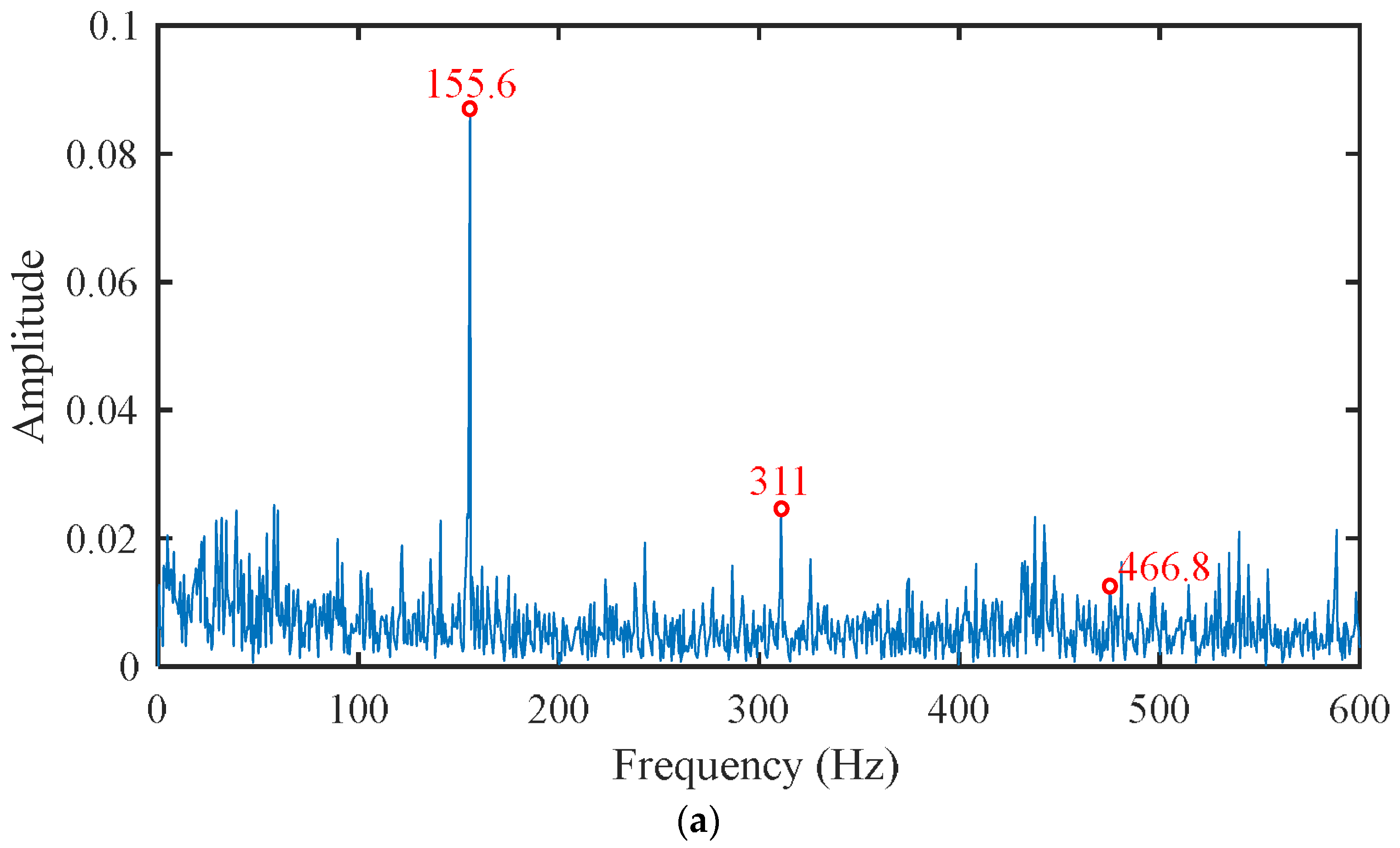
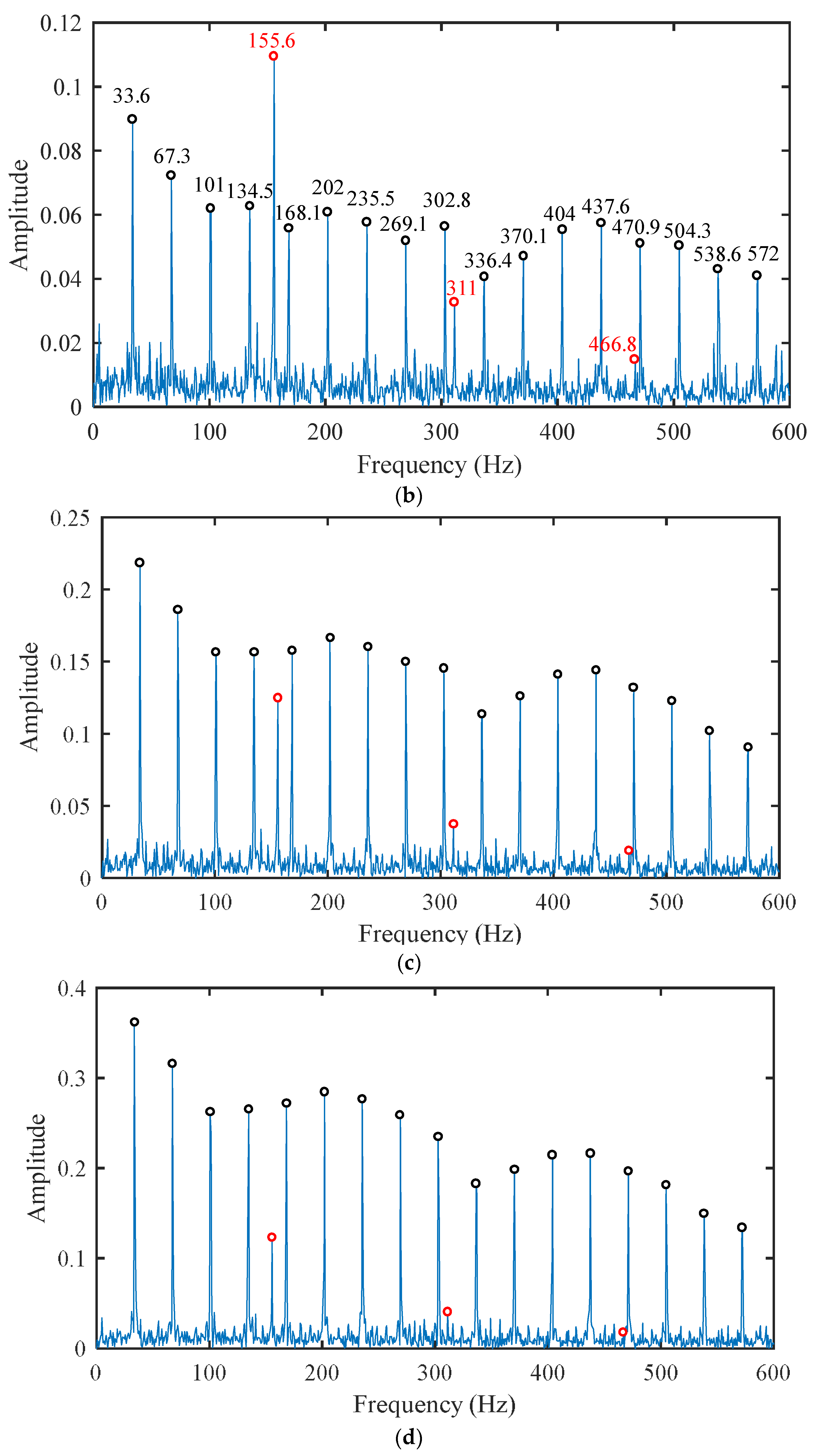
4.2. VMD-ES Analysis Results under 350 km/h

This section presents the results of the simulated axlebox acceleration by using the VMD-ES method described in Section 3. The analysis condition includes 0–50 mm length of flat at 350 km/h.

Figure 7a–f correspond to the length of the flat varying from 0 to 50 mm, respectively. The analysis frequency range is 0 Hz~600 Hz. Black dot marks represent the impact frequency of the wheel flat which is 33.6 Hz, and its relationship with the speed of vehicle is in Equation (10). Red dot marks represent interference signals unrelated to the wheel flat. According to the relationship between the length of fastener and train speed (as shown in Equation (11)), the frequency of the fastener support is 155.6 Hz which is consistent with the frequency of red dot marks. The results show that the impact frequency of the wheel flat and the frequency of the fastener support both appear in the identification results with the small flat length. As there is an increase of the flat length, the amplitude of interference frequency caused by fastener support gradually decreases. Meanwhile, the peak values in ES increase monotonically with the length of flat. It is worth noting that the irregular low amplitude frequency in ES is mainly caused by the short-wave excitation of the track irregularities especially in fault-free condition, as shown in Figure 7a. Therefore, the VMD-ES method is sensitive to the wheel flat impact and can extract the characteristic frequency of the wheel flat from the strong interference signals, which ensures the accurate identification of wheel flat.

$$f=\frac{v}{2\pi R}$$

(10)

$$f=\frac{v}{L}$$

(11)

where v is the speed of train, L is the length of fastener, and R is the wheel radius.

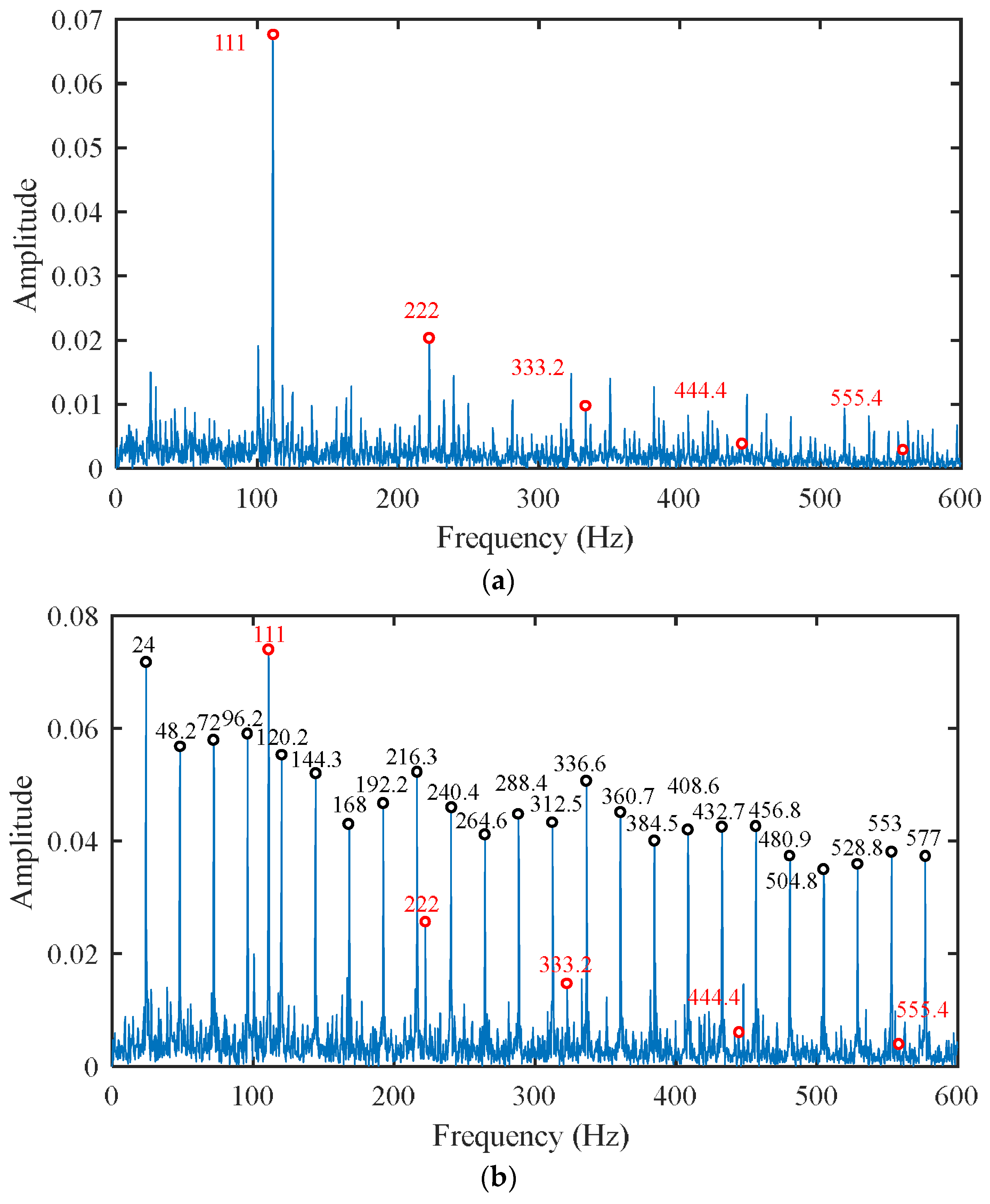
4.3. VMD-ES Analysis Results under 250 km/h

To verify the feasibility of the method at various speeds, VMD-ES was performed on partial length of the flat at 250 km/h. The results are shown in Figure 8.

According to Equations (10) and (11), the impact frequency of wheel flat and the frequency of fastener support are 24 Hz and 111 Hz at 250 km/h, which are consistent with the frequency in Figure 8. Therefore, this method has good applicability at various speeds.

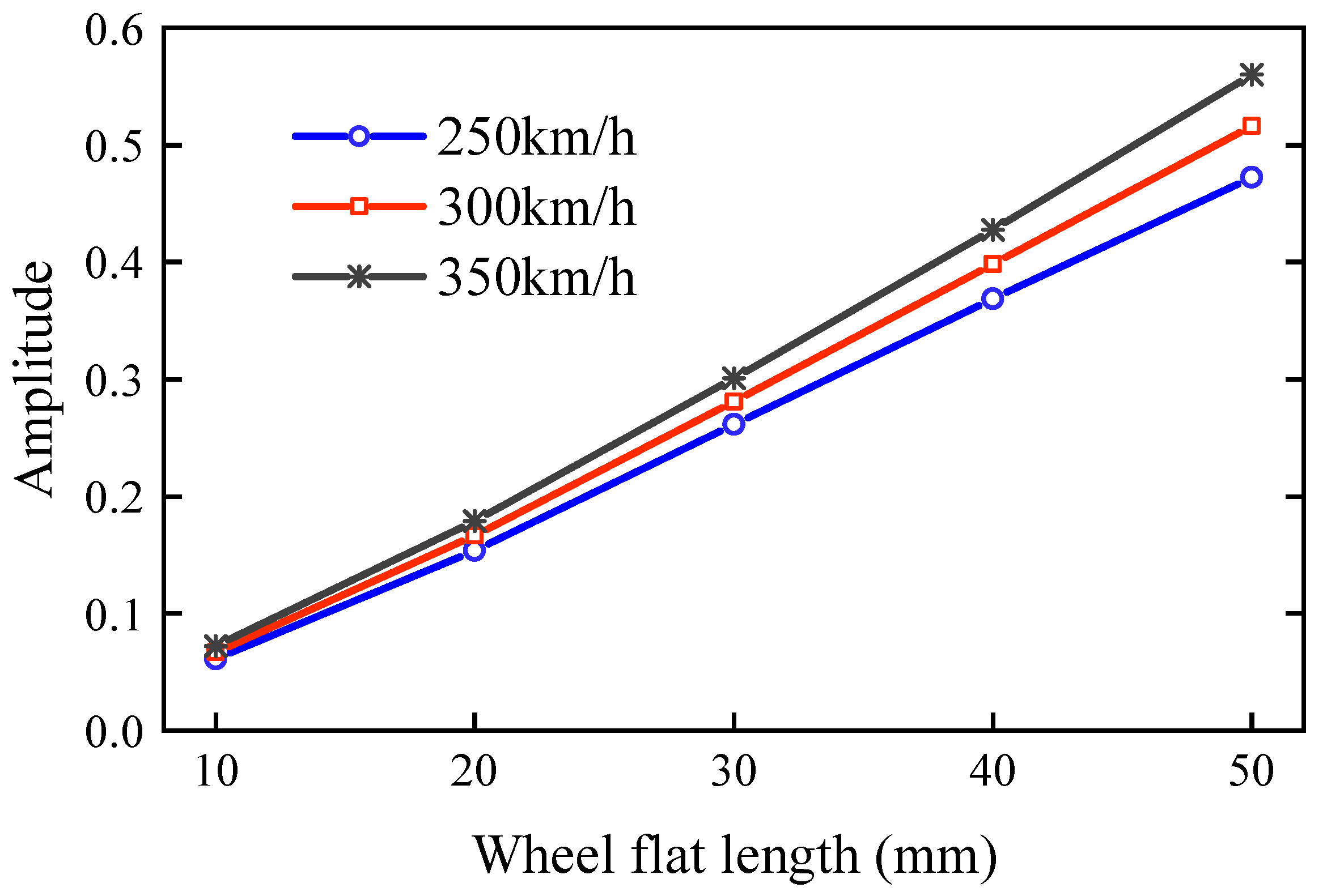
4.4. Error Analysis and Peak Value Comparison

This section presents the error between the theoretical frequency and the frequency identified by the VMD-ES method.

Table 3. The error of the wheel flat impact frequency.

Speed	Wheel Flat ImpactFrequency	1st Order	2nd Order	3rd Order	4th Order
250/(km/h−1)	Theoretical value/Hz	24	48	72	96
	Simulated value/Hz	24	48.2	72	96.2
	Error rate/%	0	0.4	0	0.2
350/(km/h−1)	Theoretical value/Hz	33.6	67.2	100.8	134.4
	Simulated value/Hz	33.6	67.3	101	134.5
	Error rate/%	0	0.1	0.2	0.07

is the error of wheel flat impact frequency, and

Table 4. The error of the fastener support frequency.

Speed	Fastener SupportFrequency	1st Order	2nd Order	3rd Order	4th Order
250/(km/h−1)	Theoretical value/Hz	111	222	333	444
	Simulated value /Hz	111	222	333.2	444.4
	Error rate/%	0	0	0.06	0.09
350/(km/h−1)	Theoretical value/Hz	155.6	311.2	466.8	622.4
	Simulated value/Hz	155.6	311	466.8	622.7
	Error rate/%	0	0.06	0	0.05

is the error of fastener support frequency. The tables only list the first four order multiple frequencies. Table 3 and Table 4 indicate that the maximum error between the simulated and theoretical value are 0.4% and 0.09%, respectively. Therefore, the accuracy of using this method for wheel flat identification is high.

Figure 9 shows the relationship between the mean amplitude of the first four multiple frequencies and the length of wheel flat at various speeds. It can be seen that the mean amplitude of the first four multiple frequencies in ES increases monotonically with the length of flat, and the difference between the mean value at the same speed expands with the increase of the wheel flat length. Hence, the mean value of the first four multiple frequencies in ES can be used to quantitatively identify the wheel flat faults.

5. Influence of the Wheel Eccentricity on Wheel Flat Identification

The wheel may occur eccentricity during the running process, and its characteristic frequency is $f_0=v/(2\pi R)$, which is consistent with the impact frequency of the wheel flat. Therefore, it is necessary to determine whether the wheel eccentricity may influence the accuracy of the wheel flat identification. Figure 10 is the result of the wheel eccentricity with 1 mm amplitude at 350 km/h by using the VMD-ES method. Figure 11 shows the results under the co-existence of the wheel eccentricity and wheel flat at the same speed (the length of flat is 14 mm and the amplitude of wheel eccentricity is 1 mm). The results show that only the dominant frequency (33.6 Hz) is presented in ES under the wheel eccentricity. Meanwhile, in the case of co-existence of the wheel eccentricity and flat, the multiple frequency generated by the wheel flat is reflected in ES. The mean amplitude of the first four multiple frequencies is almost the same with the value corresponding to the length of a 14 mm flat in Figure 9. Therefore, the proposed method has good ability in wheel flat identification under the co-existence of the wheel eccentricity and flat.

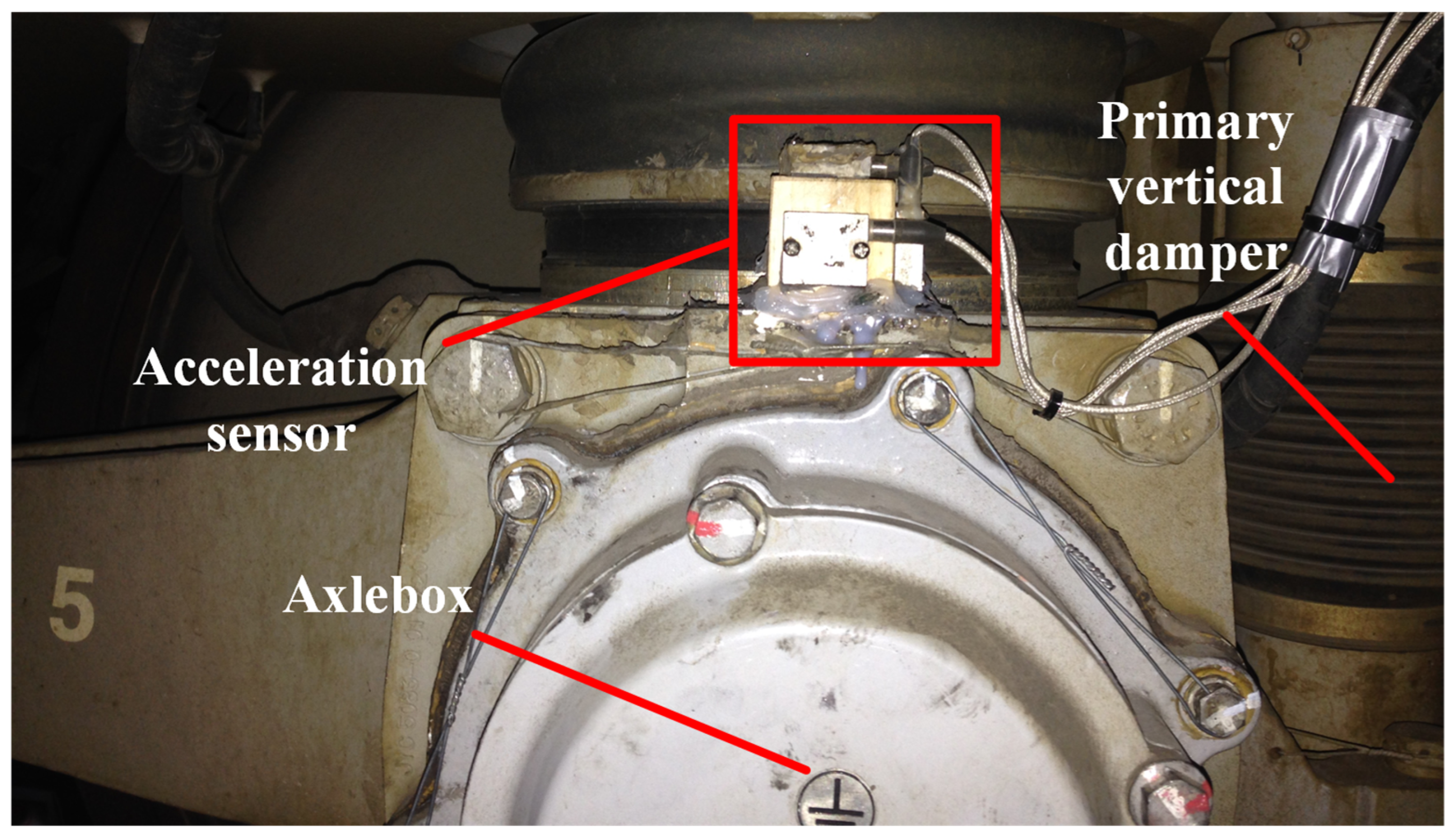
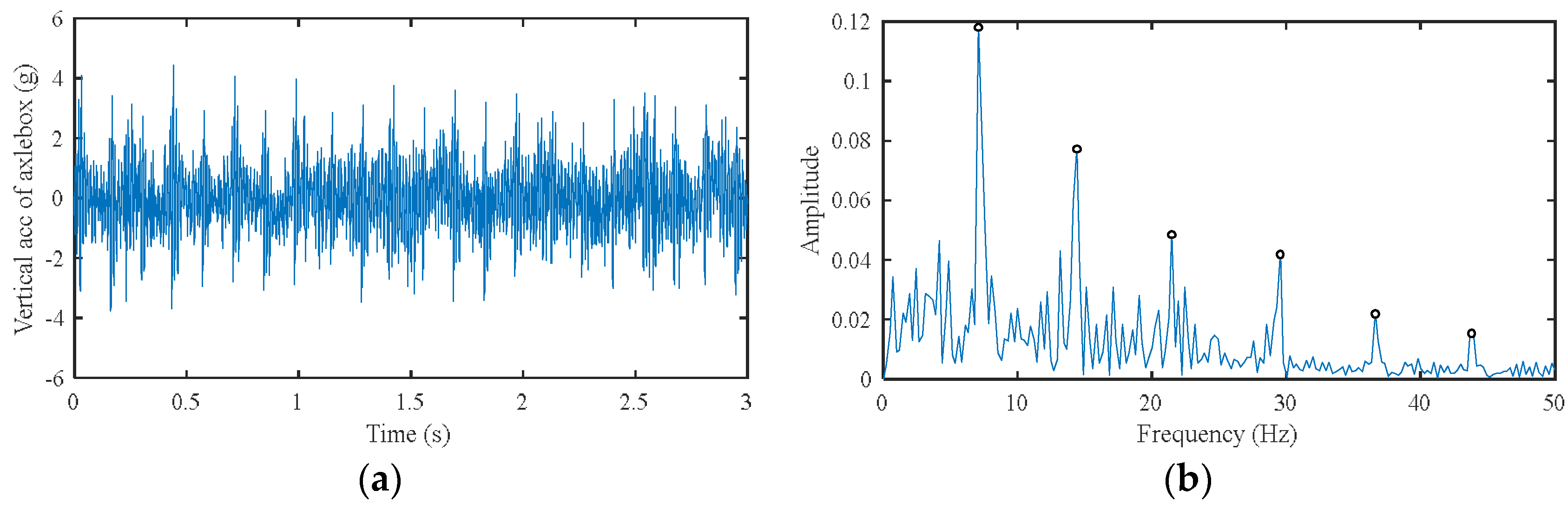
6. Field Test Validation

In this section, the axlebox acceleration was measured from the in-service vehicle on a certain line at 75 km/h. The sampling frequency of the measured data is 4 kHz. Figure 12 illustrates the placement of the axlebox acceleration sensor.

The measured data with the wheel flat is analyzed by the proposed VMD-ES method; Figure 13a is the vertical axlebox acceleration signal with the length of 16 mm wheel flat and Figure 13b is the analysis of results using this method. The multiple frequency of the wheel flat impact are clearly represented in the results (the impact frequency is 7.2 Hz) which is consistent with the rule of the dynamics simulation. In the measured data, the mean value of the first four multiple frequencies under 16 mm wheel flat length is 0.075. Meanwhile, the value in Figure 9 is 0.078. The error rate between the simulation and measurement is 4%. The results verify the accuracy of the established vehicle dynamic model. Therefore, the proposed VMD-ES method can detect the wheel flat fault from the strong interference signal.

7. Conclusions

This work proposes an on—board monitoring method based on the axlebox acceleration using the VMD—ES method. A three—dimensional vehicle—track coupled dynamic model verified by field test was established to simulate the axlebox acceleration of a high—speed railway. The simulation and field test results show that the VMD–ES method accurately extracts the impact characteristics of the wheel flat and can quantitatively identify the wheel flat faults at various speeds. Based on the results, the following conclusions can be drawn:

(1)

The axlebox acceleration includes strong interference signal excited by the rail and wheel which influences the accurate identification of the wheel flat. The results show that the proposed VMD–ES method accurately extracts the characteristic frequency of the wheel flat from complex frequency components. Meanwhile, the mean amplitude of the first four multiple frequency increases monotonically with the length of flat in ES. Therefore, the VMD–ES method can be applied to quantitatively identify the wheel flat faults at various speeds.

(2)

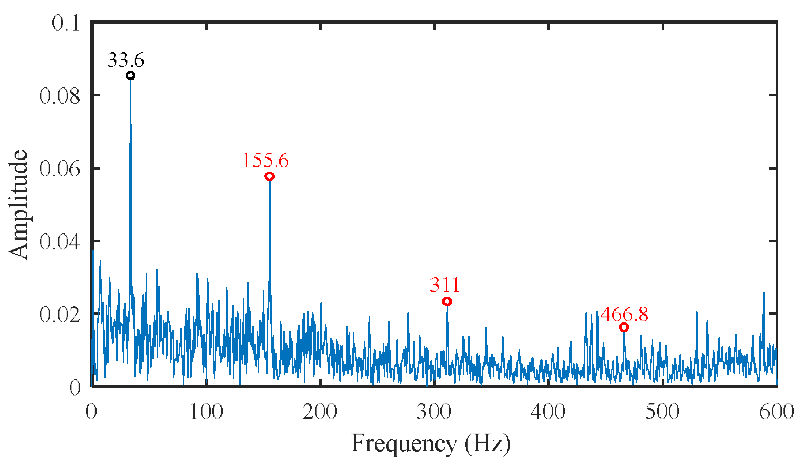
In the case of the wheel eccentricity, only the dominant frequency (33.6 Hz) is presented in the results of ES. At the co-existence of the wheel eccentricity and flat, the VMD–ES method can accurately extract the multiple frequency of the wheel flat. The method has good adaptability in wheel flat identification; wheel eccentricity has no influence on the detection.

(3)

The field test is carried out to verify the accuracy of the method. The results of the field test are consistent with the simulation results, which reflect the correctness of the established vehicle-track coupled dynamics model, and the feasibility of the wheel flat identification by using this method.

In this paper, the wheel flat detection is investigated in detail by using the VMD-ED method. The results show that the method can quantitatively identify the wheel flat faults at various speeds. Machine learning methods will be combined with advanced signal processing techniques to identify the wheel flat in our future work.

References

1. Wang, Z.; Allen, P.; Mei, G.; Yin, Z.; Cheng, Y.; Zhang, W. Dynamic characteristics of a high-speed train gearbox in the vehicle–track coupled system excited by wheel defects. Proc. Inst. Mech. Eng. Part F J. Rail Rapid Transit 2020, 234, 1210–1226. [Google Scholar] [CrossRef]
2. Wang, Z.; Mo, J.; Gebreyohanes, M.Y.; Wang, K.; Wang, J.; Zhou, Z. Dynamic response analysis of the brake disc of a high-speed train with wheel flats. Proc. Inst. Mech. Eng. Part F J. Rail Rapid Transit 2022, 236, 593–605. [Google Scholar] [CrossRef]
3. Masoudi Nejad, R.; Noroozian Rizi, P.; Zoei, M.S.; Aliakbari, K.; Ghasemi, H. Failure Analysis of a Working Roll Under the Influence of the Stress Field Due to Hot Rolling Process. J. Fail. Anal. Prev. 2021, 21, 870–879. [Google Scholar] [CrossRef]
4. Bian, J.; Gu, Y.; Murray, M.H. A dynamic wheel-rail Impact analysis of rail rail track under Wheel flat by finite element analysis. Veh. Syst. Dyn. 2013, 51, 784–797. [Google Scholar] [CrossRef] [Green Version]
5. Bernal, E.; Spiryagin, M.; Cole, C. Onboard condition monitoring sensors, systems and techniques for freight railway vehicles: A Review. IEEE Sens. J. 2019, 19, 4–24. [Google Scholar] [CrossRef]
6. Mosleh, A.; Montenegro, P.A.; Costa, P.A.; Calçada, R. Railway vehicle wheel flat detection with multiple records using spectral kurtosis analysis. Appl. Sci. 2021, 11, 4002. [Google Scholar] [CrossRef]
7. Alemi, A.; Corman, F.; Pang, Y.; Lodewijks, G. Reconstruction of an informative railway wheel defect signal from wheel-rail contact signals measured by multiple wayside sensors. Proc. Inst. Mech. Eng. Part F J. Rail Rapid Transit 2019, 233, 49–62. [Google Scholar] [CrossRef] [Green Version]
8. Cao, W.; Zhang, S.; Bertola, N.J.; Smith, I.F.C.; Koh, C.G. Time series data interpretation for ‘wheel-flat’ identification including uncertainties. Struct. Health Monit. 2019. [Google Scholar] [CrossRef]
9. Salzburger, H.J.; Schuppmann, M.; Li, W.; Gao, X. In-motion ultrasonic testing of the tread of high-speed railway wheels using the inspection system AUROPA III. Insight—Non-Destructive Test. Cond. Monit. 2009, 51, 370–372. [Google Scholar]
10. Brizuela, J.; Ibañez, A.; Nevado, P.; Fritsch, C. Railway wheels flat detector using Doppler effect. Phys. Procedia 2010, 3, 811–817. [Google Scholar] [CrossRef] [Green Version]
11. Brizuela, J.; Fritsch, C.; Ibáñez, A. Railway wheel-flat detection and measurement by ultrasound. Transp. Res. Part C Emerg. Technol. 2011, 19, 975–984. [Google Scholar] [CrossRef]
12. Lai, C.C.; Kam, J.C.P.; Leung, D.C.C.; Lee, T.K.Y.; Tam, A.Y.M.; Ho, S.L.; Tam, H.Y.; Liu, M.S.Y. Development of a fiber-optic sensing system for train vibration and train weight measurements in Hong Kong. J. Sens. 2012, 2012, 1–7. [Google Scholar] [CrossRef] [Green Version]
13. Tam, H.Y.; Liu, S.Y.; Guan, B.O.; Chung, W.H.; Chan, T.H.T.; Cheng, L.K. Fiber Bragg Grating sensors for structural and railway applications. In Proceedings of the SPIE-The International Society for Optical Engineering, Beijing, China, 8 November 2004; pp. 85–97. [Google Scholar]
14. Wei, C.; Lai, C.; Liu, S.; Chung, W.H.; Ho, T.K.; Tam, H.; Ho, S.L.; McCusker, A.; Kam, J.; Lee, K.Y. A Fiber Bragg Grating sensor system for train axle counting. IEEE Sens. J. 2010, 10, 1905–1912. [Google Scholar]
15. Filograno, M.L.; Rodriguez-Barrios, A.; González-Herraez, M.; Corredera, P.; Martín-López, S.; Rodríguez-Plaza, M.; Andrés-Alguacil, A. Real-time monitoring of railway traffic using Fiber Bragg Grating sensors. IEEE Sens. J. 2012, 12, 85–92. [Google Scholar] [CrossRef]
16. Alemi, A.; Corman, F.; Lodewijks, G. Condition monitoring approaches for the detection of railway wheel defects. Proc. Inst. Mech. Eng. Part F J. Rail Rapid Transit 2017, 231, 961–981. [Google Scholar] [CrossRef] [Green Version]
17. Liang, B.; Iwnicki, S.; Ball, A.; Young, A.E. Adaptive noise cancelling and time–frequency techniques for rail surface defect detection. Mech. Syst. Signal Process. 2014, 54–55, 41–51. [Google Scholar] [CrossRef] [Green Version]
18. Bosso, N.; Gugliotta, A.; Zamperi, N. Wheel flat detection algorithm for onboard diagnostic. Measurement 2018, 123, 193–202. [Google Scholar] [CrossRef]
19. Shim, J.; Kim, G.; Cho, B.; Koo, J. Application of vibration signal processing methods to detect and diagnose wheel flats in railway vehicles. Appl. Sci. 2021, 11, 2151. [Google Scholar] [CrossRef]
20. Shi, D.; Ye, Y.; Gillwal, M.; Hecht, M. Designing a lightweight 1D convolutional neural network with Bayesian optimization for wheel flat detection using carbody accelerations. Int. J. Rail Transp. 2020, 9, 311–341. [Google Scholar] [CrossRef]
21. Bernal, E.; Spiryagin, M.; Cole, C. Wheel flat analogue fault detector verification study under dynamic testing conditions using a scaled bogie test rig. Int. J. Rail Transp. 2021, 10, 177–194. [Google Scholar] [CrossRef]
22. Huang, N.E.; Shen, Z.; Long, S.R.; Wu, M.C.; Shih, H.H.; Zheng, Q.; Yen, N.; Tung, C.C.; Liu, H.H. The empirical mode decomposition and the hilbert spectrum for nonlinear and non-stationary time series analysis. Proc. R. Soc. Lond. Ser. A Math. Phys. Eng. Sci. 1998, 454, 903–995. [Google Scholar] [CrossRef]
23. Li, Y.; Zuo, M.J.; Lin, J.; Liu, J. Fault detection method for railway wheel flat using an adaptive multiscale morphological filter. Mech. Syst. Signal Process. 2017, 84, 642–658. [Google Scholar] [CrossRef]
24. Li, Y.; Liu, J.; Wang, Y. Railway wheel flat detection based on improved empirical mode decomposition. Shock Vib. 2016, 2016, 4879283. [Google Scholar] [CrossRef]
25. Chen, S.; Wang, K.; Chang, C.; Xie, B.; Zhai, W. A two-level adaptive chirp mode decomposition method for the railway wheel flat detection under variable-speed conditions. J. Sound Vib. 2021, 498, 115963. [Google Scholar] [CrossRef]
26. Dragomiretskiy, K.; Zosso, D. Variational mode decomposition. IEEE Trans. Signal Process. 2014, 62, 531–544. [Google Scholar] [CrossRef]
27. Zhu, S.; Xia, H.; Peng, B.; Zio, E.; Wang, Z.; Jiang, Y. Feature extraction for early fault detection in rotating machinery of nuclear power plants based on adaptive VMD and Teager energy operator. Ann. Nucl. Energy 2021, 160, 108392. [Google Scholar] [CrossRef]
28. Jin, Z.; He, D.; Wei, Z. Intelligent fault diagnosis of train axle box bearing based on parameter optimization VMD and improved DBN. Eng. Appl. Artif. Intel. 2022, 110, 104713. [Google Scholar] [CrossRef]
29. Li, H.; Liu, T.; Wu, X.; Chen, Q. An optimized VMD method and its applications in bearing fault diagnosis. Measurement 2020, 166, 108185. [Google Scholar] [CrossRef]
30. Bernal, E.; Spiryagin, M.; Cole, C. Wheel flat detectability for Y25 railway freight wagon using vehicle component acceleration signals. Veh. Syst. Dyn. 2020, 58, 1893–1913. [Google Scholar] [CrossRef]
31. Zhai, W. Vehicle-Track Coupled Dynamics Theory and Applications; Springer: Singapore, 2020. [Google Scholar]
32. Wu, T.; Thompson, D. A hybrid model for the noise generation due to railway wheel flats. J. Sound Vib. 2002, 251, 115–139. [Google Scholar] [CrossRef]
33. Yang, J.; Zhou, C.; Li, X. Research on Fault Feature Extraction Method Based on Parameter Optimized Variational Mode Decomposition and Robust Independent Component Analysis. Coatings 2022, 12, 419. [Google Scholar] [CrossRef]
Figure 1. Vehicle-track coupled dynamics model: (a) lateral view; (b) front view.
Applsci 12 06837 g001
Figure 2. Simulation and verification of the axlebox acceleration.
Applsci 12 06837 g002
Figure 3. Motion of the flat wheel.
Applsci 12 06837 g003
Figure 4. Illustration of the wheel flat: (a) wheel flat model; (b) the relationship between the depth and length of the wheel flat.
Applsci 12 06837 g004
Figure 5. The flow chart of VMD-Envelope spectrum method.
Applsci 12 06837 g005
Figure 6. The result of VMD.
Applsci 12 06837 g006
Figure 7. The results of VMD-ES at 350 km/h: (a) fault-free condition; (b) wheel flat length of 10 mm; (c) wheel flat length of 20 mm; (d) wheel flat length of 30 mm; (e) wheel flat length of 40 mm; (f) wheel flat length of 50 mm.
Applsci 12 06837 g007aApplsci 12 06837 g007bApplsci 12 06837 g007c
Figure 8. The results of VMD-ES at 250 km/h: (a) fault-free condition; (b) wheel flat length of 10 mm.
Applsci 12 06837 g008
Figure 9. The relationship between the mean amplitude of the first four orders and the length of wheel flat.
Applsci 12 06837 g009
Figure 10. The results of wheel eccentricity.
Applsci 12 06837 g010
Figure 11. The results of the co-existence of wheel eccentricity and wheel flat.
Applsci 12 06837 g011
Figure 12. The placement of the axlebox acceleration sensor.
Applsci 12 06837 g012
Figure 13. Field test: (a) the measured data; (b) The results of the measured data based on the VMD-ES method.
Applsci 12 06837 g013