
GAN-Based Image Dehazing for Intelligent Weld Shape Classification and Tracing Using Deep Learning


Abstract
:1. Introduction
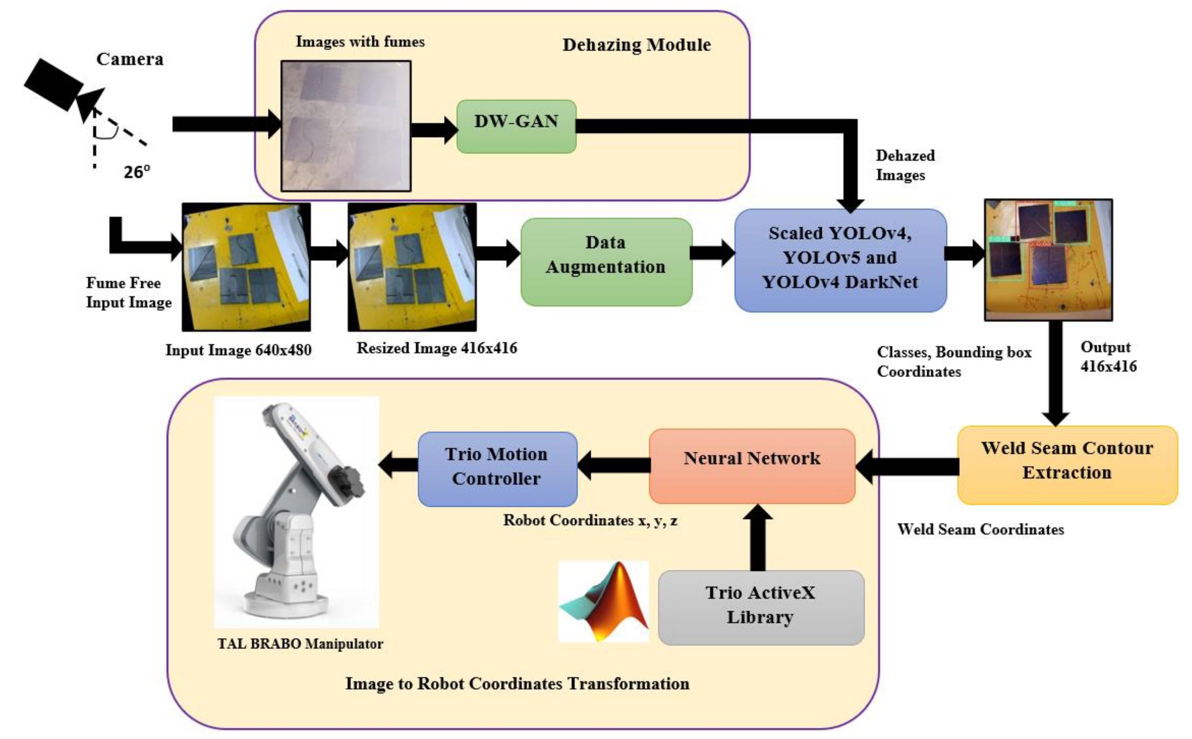
- Create a real-time weld dataset made up of actual weld plates with a variety of different weld shapes;
- Remove weld fumes using the DW-GAN;
- Train the dataset with genetic algorithm-based different YOLO approaches, such as Scaled YOLOv4, YOLOv5, and YOLOv4 DarkNet;
- Determine the contours of various weld seam shapes using image processing;
- Convert pixel coordinates to robot coordinates using a Backpropagation Neural Network model;
- Perform real-time weld seam detection for tracing the weld seam shapes using a live 2D camera.
2. Methods
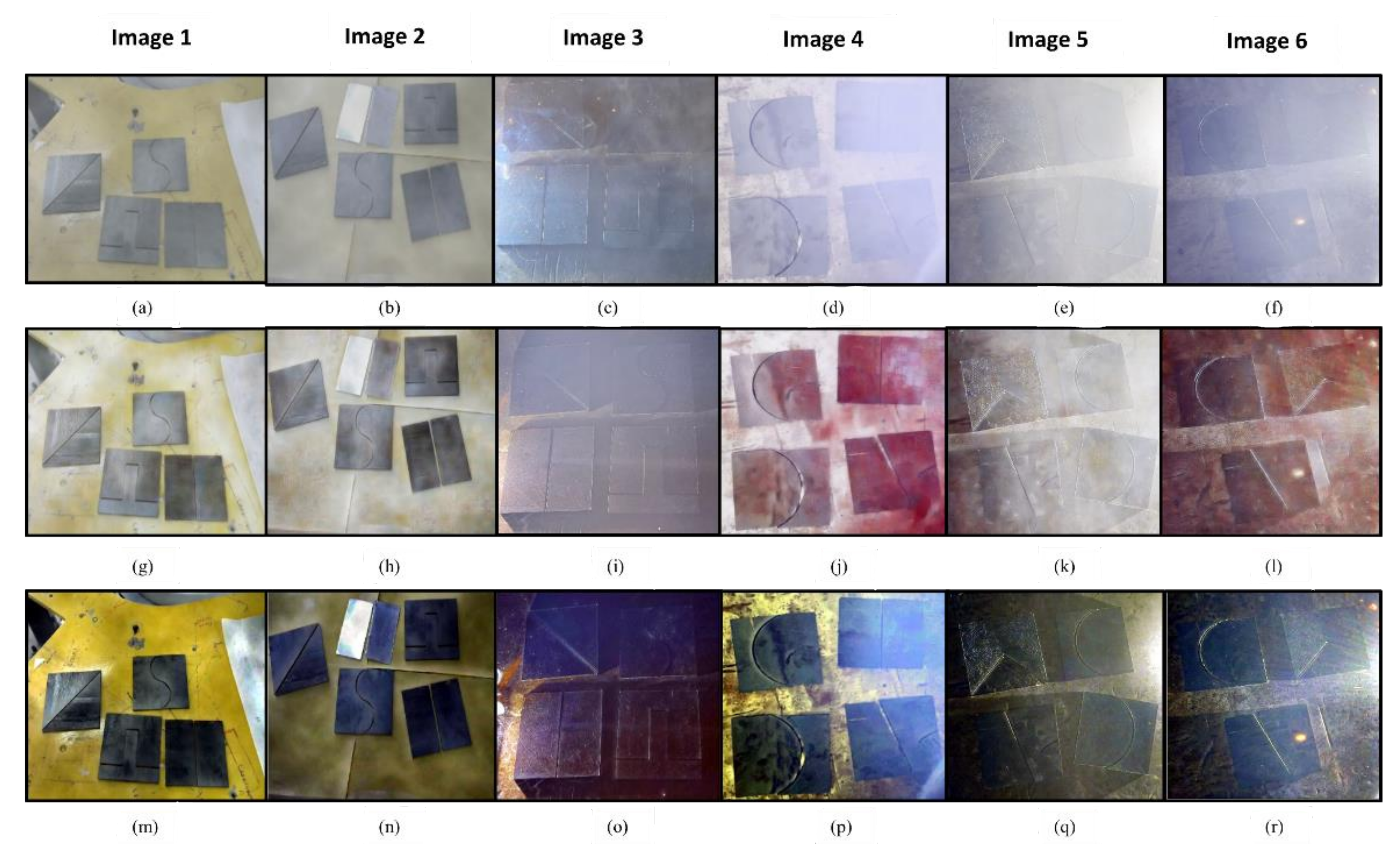
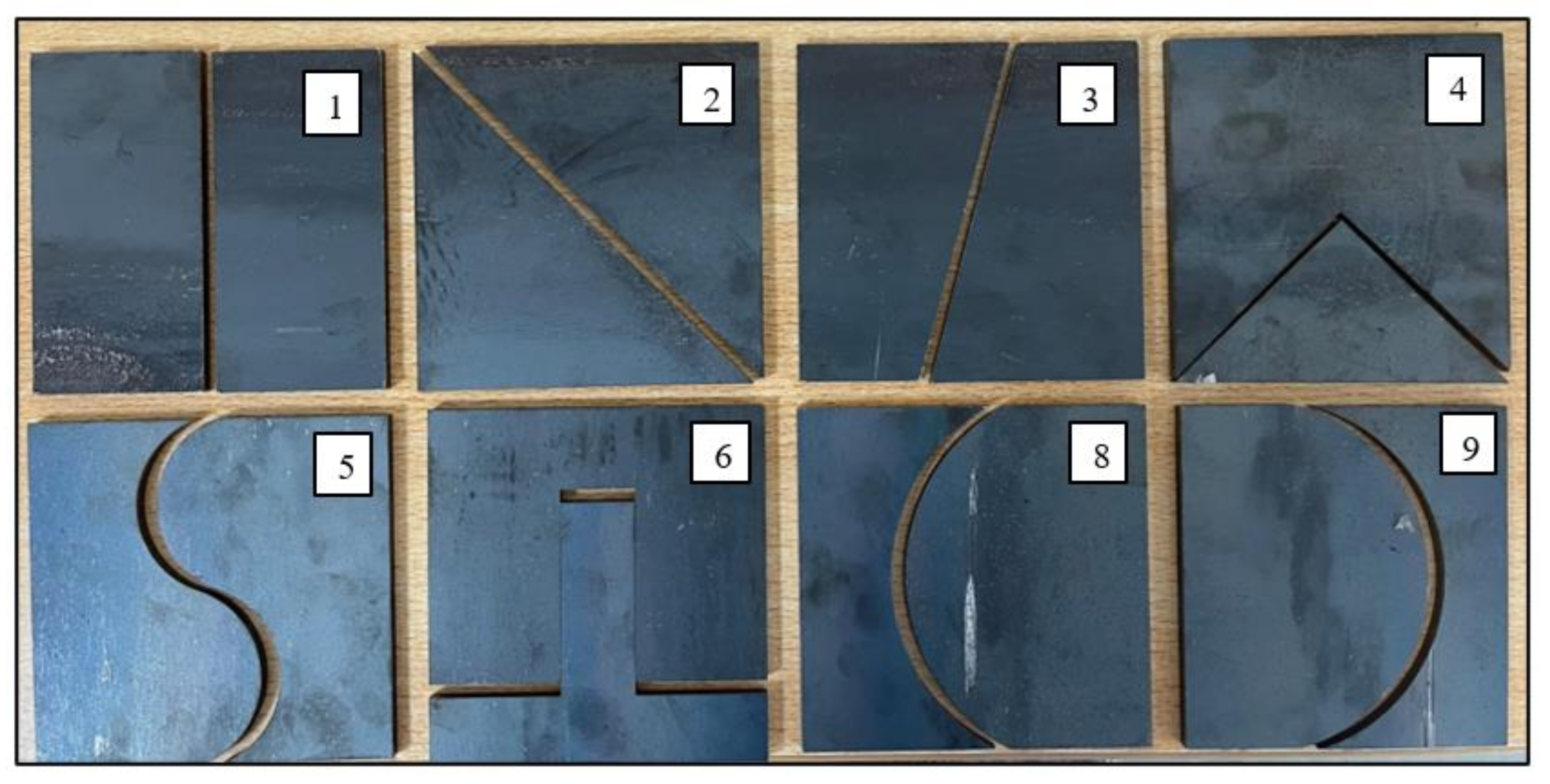
2.1. Dataset Preparation
2.2. Dehazing Techniques for Weld Fume Removal
2.2.1. DW-GAN Architecture
2.2.2. DWT Branch Using U-Net
2.2.3. Knowledge Adaption Branch Using ImageNet and Res2Net
Discriminator
2.3. Theoretical Background of YOLO Architecture
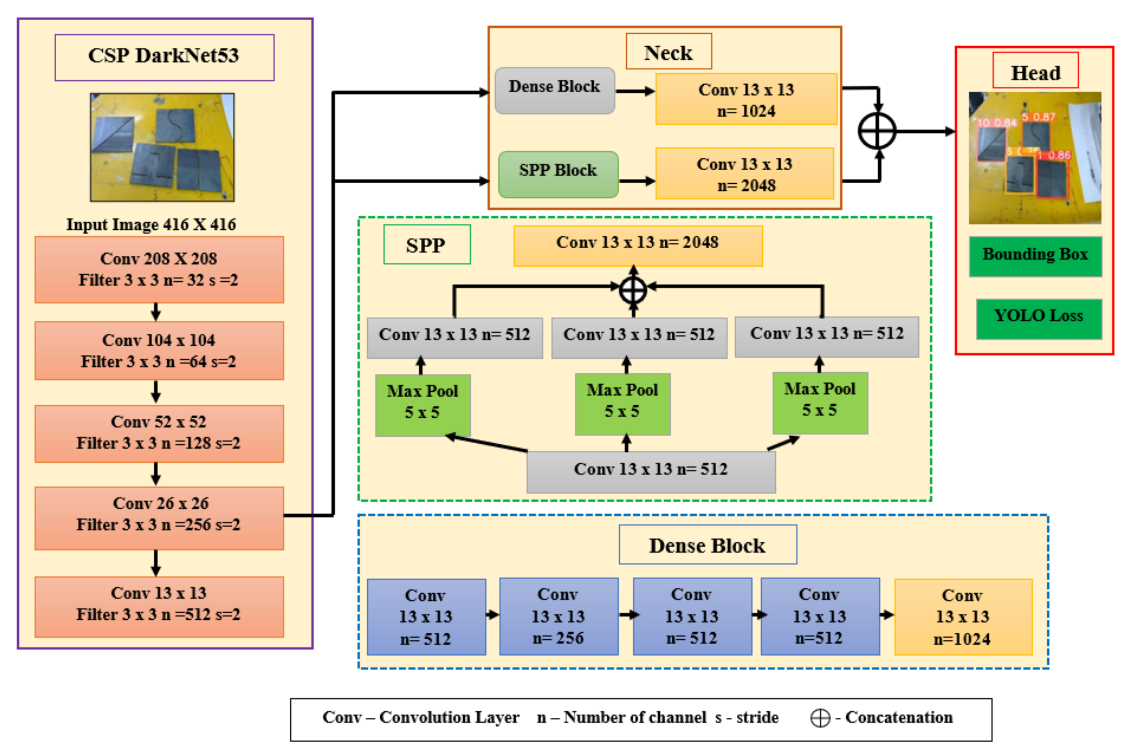
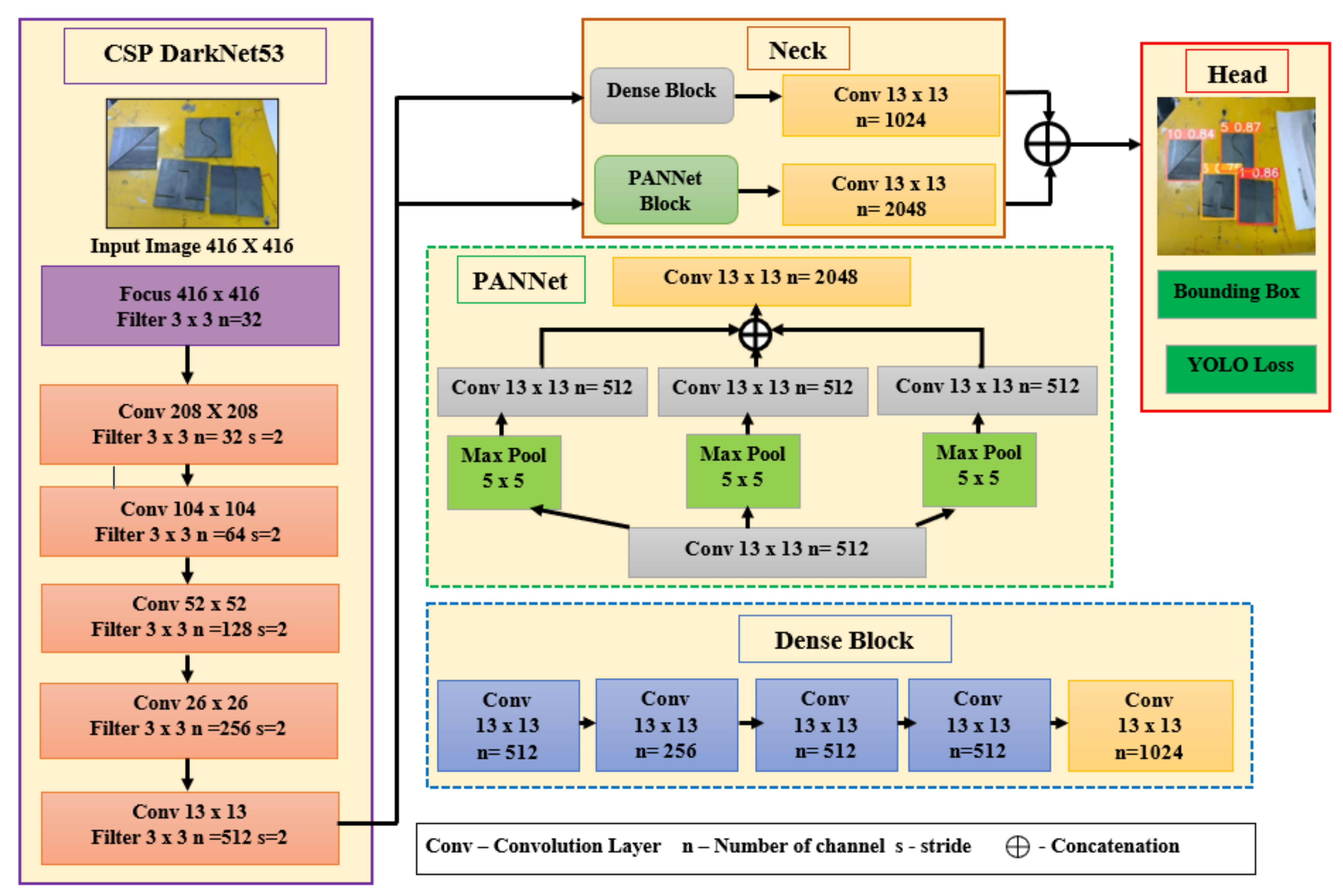
2.3.1. YOLOv4 Architecture
2.3.2. YOLOv5 Architecture
| Algorithm 1 Pseudocode of Weld Seam Detection using YOLO Algorithms |
| Begin Input: weld images I_weld, Bounding box coordinates x, y width Bw, height Bh Output: Class probabilities Pc and Predicted Bounding box coordinates Data partition: I_weld = I_train (60%)+I_test (20%)+I_validation (20%) Initialize no of epochs N = 200 batch_size = 16 Resize the image to 416 × 416 Generation = 100 Mutation_probability = 0.9 Sigma = 0.2 for i = 1 to generation for j = 1 to batch_size Load pretrained weights w Load yolo configuration files Run GA to obtain best hyperparameter values end for end for Training phase: for i = 1 to N Load optimized weights and biases Load optimized yolo training parameters from GA Perform training on I_train end for save checkpoint weights.ckpt Testingphase: for each videoframe do I_test = capture(videoframe) predict y = f(Pc, Bw, Bh, Bx, By) No of predictions = 13 × 13 × (5*3 + c) Display class c and Pc end for end |
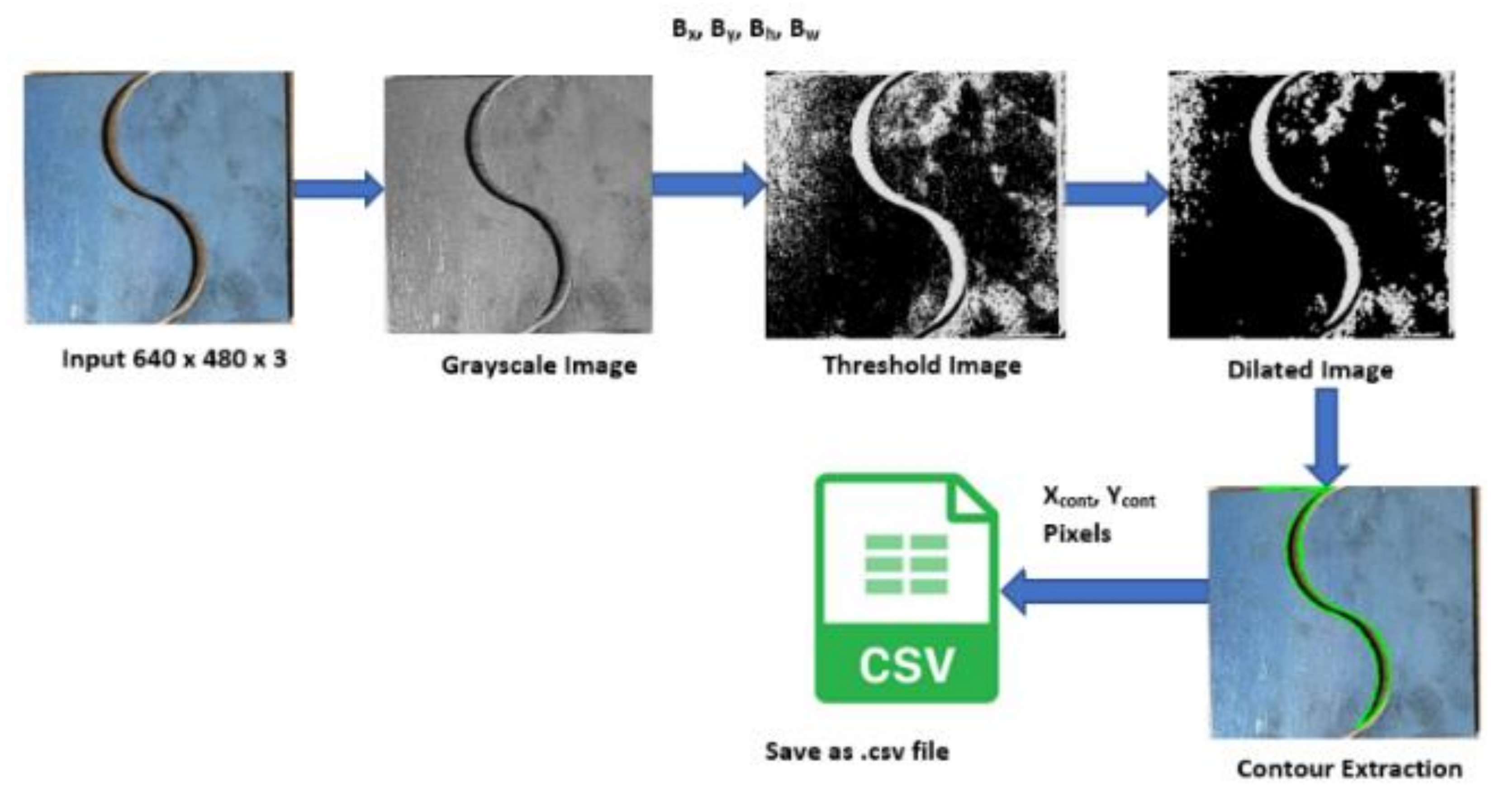
2.4. Contour Detection for the Extraction of Weld Seams
| Algorithm 2 Pseudocode of Contour Extraction of Weld Seam |
| Begin Input:Image 640 × 480 × 3; I = f (u, v,3) Output:Contour Points C = (xcont, ycont) fori = 1 to n Read test weld image or live camera image I = f(u, v,3) Extract the individual channels from RGB image, R = I (:, :,1); G = I (:, :,2); B = I (:, :,3); Grayscale Conversion, grayImage = (R+G+B)/3 Perform Inverted Binary Image thresholding, set T = 100 iff (x, y) > T then f (x, y) = 0 else f (x, y) = 255 end if Perform erosion and dilation Find contours using C = cv2.findContours() Draw contours using C pixel points end for Save contour points C to .csv end |
3. Evaluation of Weld Seam Detection
4. Results and Discussion
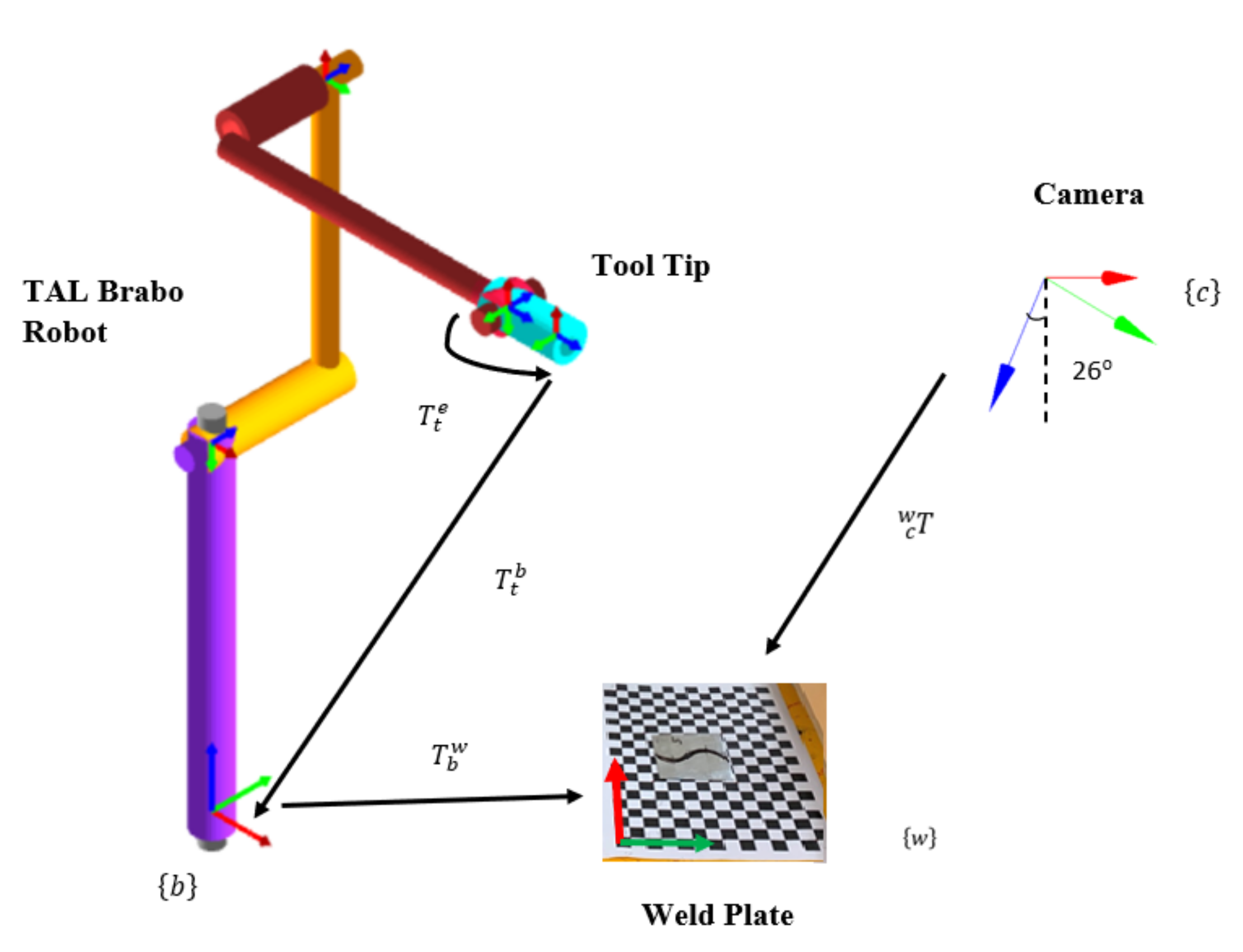
4.1. Experimental Setup for Real-Time Weld Seam Tracing
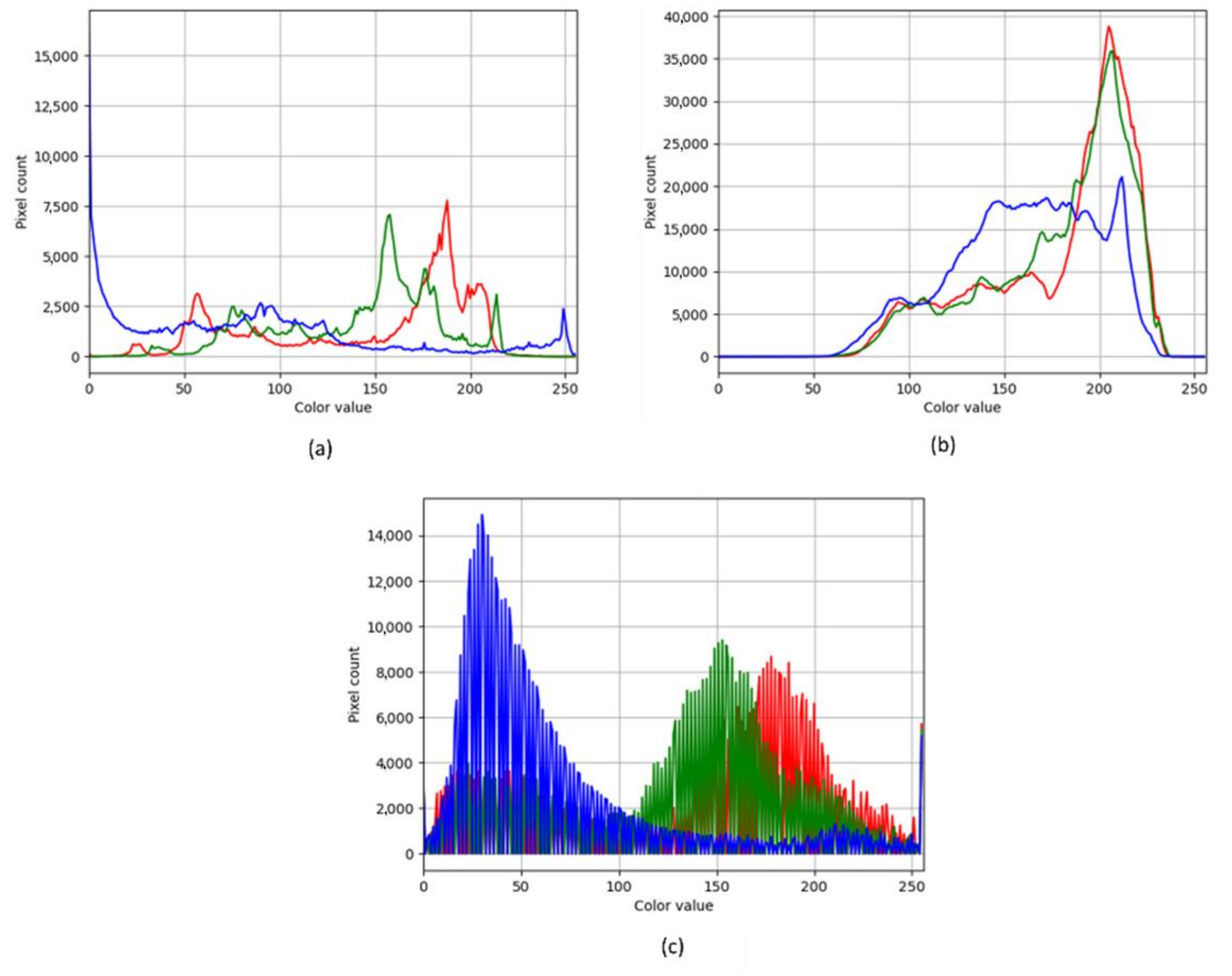
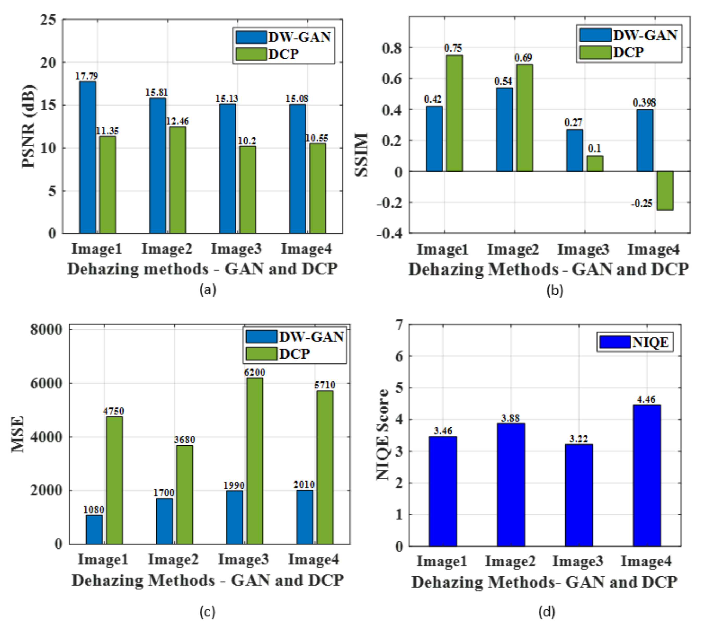
4.2. Weld Fume Removal Using GAN
4.3. Training Phase of Weld Seam Detection using YOLO Algorithms
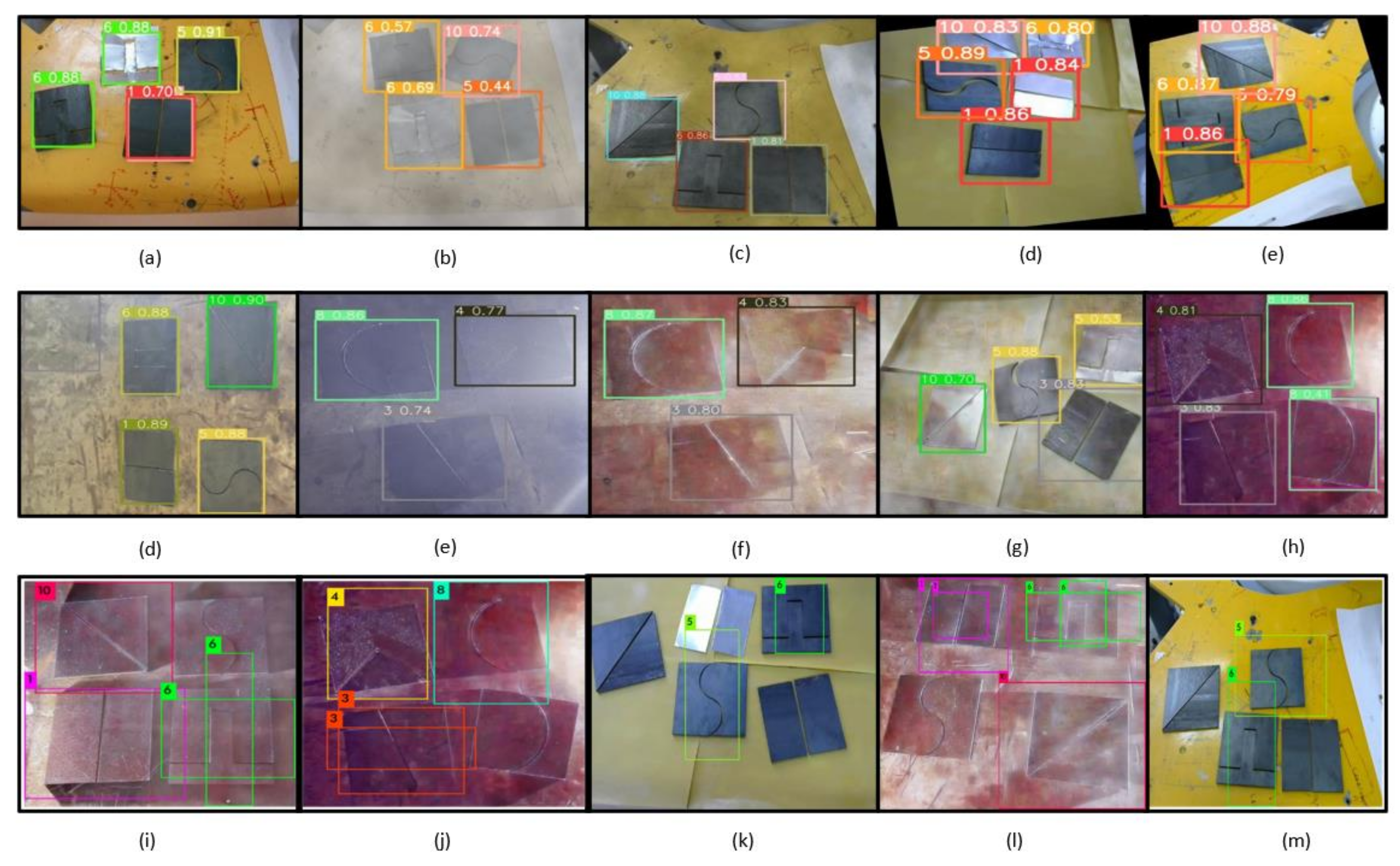
4.4. Testing Phase of Weld Seam Detection Using YOLO Algorithms
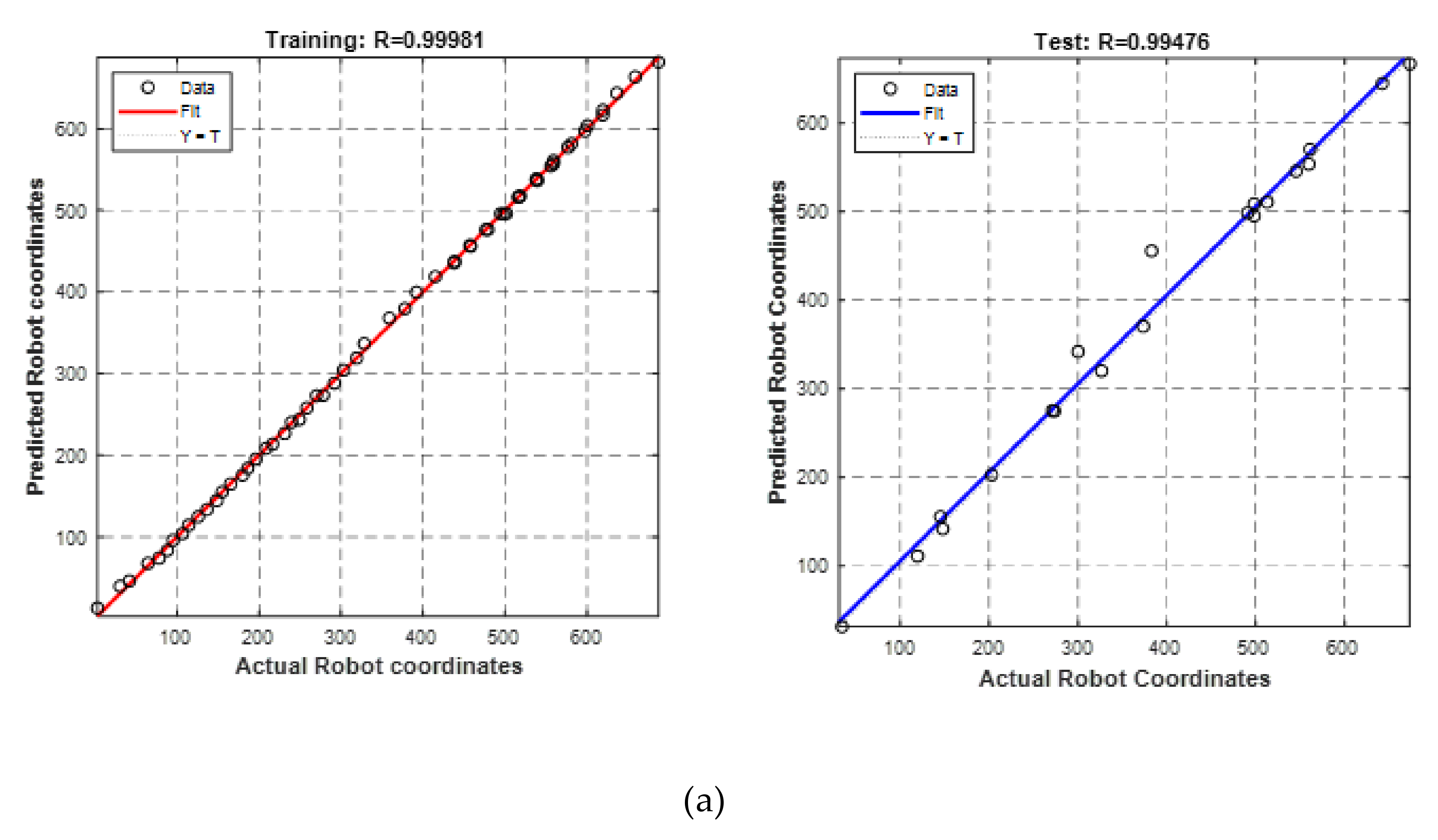
4.5. Coordinate Transformation Using the Artificial Neural Network
4.6. Comparison of Proposed Methodology with Previous Works
5. Conclusions
- Real-time weld datasets were collected, and were made of actual weld plates of mild steel. The total dataset for training the model comprised 2286 images with an image size of 416 × 416;
- The weld fumes generally affected the detection performance; hence, DW-GAN was implemented to remove the weld fumes. The performance was compared with the conventional DCP method, and it was found that DW-GAN performed better for removing the fumes with PSNR 15.95 dB and SSIM 0.407. The inference time of DW-GAN was faster by 9.6 ms compared to DCP;
- With the help of the YOLOv5 algorithm, the accurate and fast detection of weld seam shapes was realized with an overall inference speed of 0.0096 s, which was faster than Scaled YOLOv4 and YOLOv4 DarkNet. Additionally, the detection accuracy of YOLOv5 was 95%, with 96.7% precision, 96% recall, and 98.7% F1 score. The total loss of YOLOv5 was 0.043, whereas this was high for YOLOv4 DarkNet with the value of 0.959;
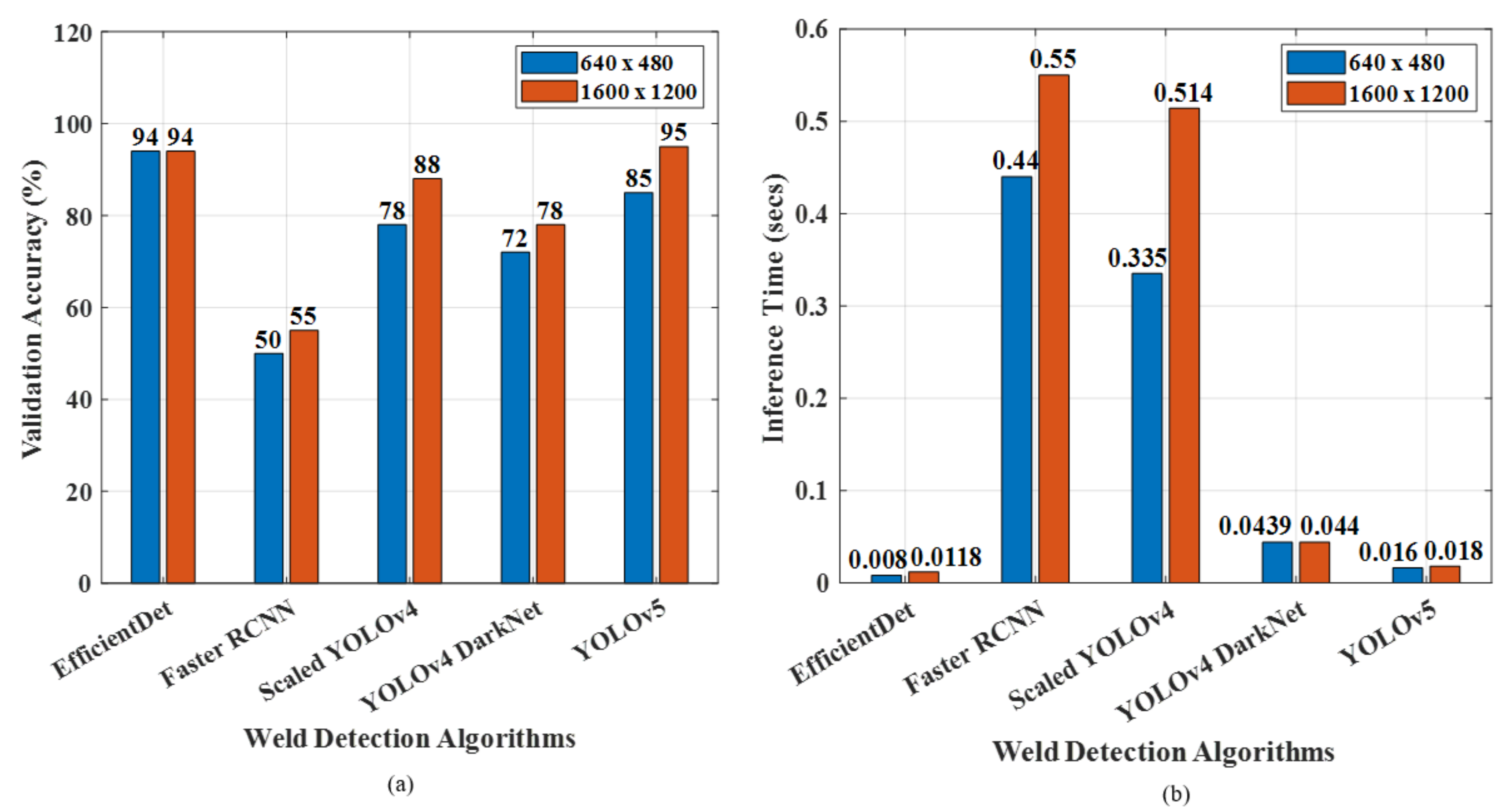
- The YOLO algorithms were compared with Faster RCNN and EfficientDet and it was inferred that EfficientDet’s performance was similar to YOLOv5, and they outperformed other deep learning algorithms. The performance of the deep learning models was tested with different image sizes to validate the generalization ability, and weld plate detection was experimentally verified using live 2D camera images. The total processing time taken for YOLOv5 was just 6.426 s, which was less than that of the other deep learning methods;
- An ablation study was performed to show the contribution of modules used in this work. The performance was analyzed in terms of validation accuracy and total time for the entire process. It was found that GAN played a major contribution in weld fume removal because accuracy was improved after dehazing;
- The optimal combination of training parameters for NN was analyzed in terms of MSE, regression value, and RMSE, and it was found that the 50-25-25 training–validation–testing ratio with trainsscg was optimal for the efficient mapping of pixels into robot coordinates. The NN model made the coordinate transformation between the camera and the robot simpler, and this technique could be used in any machine vision application effectively and efficiently;
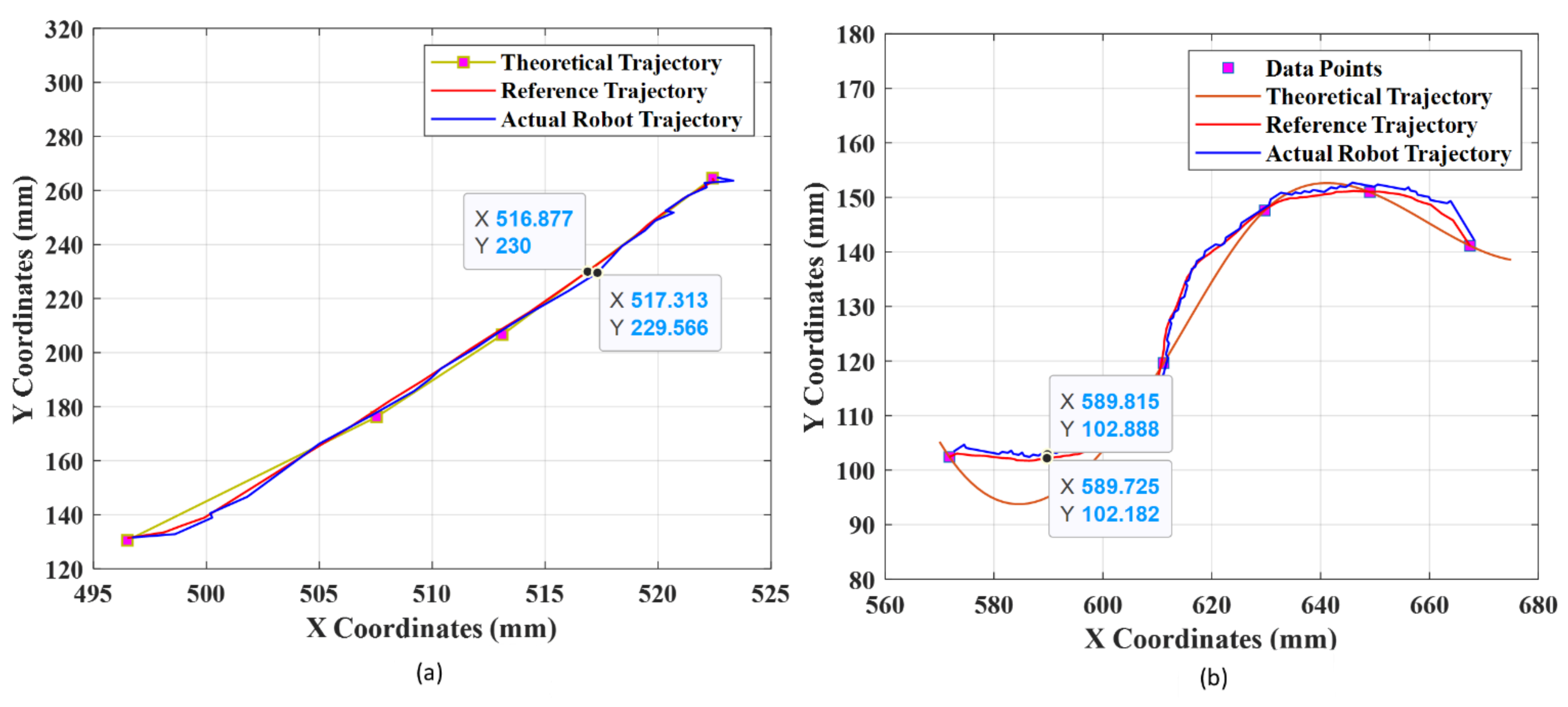
- The contours present in the weld images were detected successfully and were sent to the robot using the trained NN model for simulated robotic welding via MATLAB. It was inferred that the accurate robot coordinates were obtained from the NN, which was helpful for accurate real-time weld shape tracing. The average tracking error was found to be less than 0.3 mm for all of the shapes.
Author Contributions
Funding
Institutional Review Board Statement
Informed Consent Statement
Data Availability Statement
Acknowledgments
Conflicts of Interest
Nomenclature
| Symbol | Description |
| , , , and | Low pass and high pass filters |
| Total loss of DW-GAN | |
| Smooth loss | |
| Multi-scale structural similarity index loss | |
| Perceptual loss | |
| Adversarial loss | |
| , | Weighting factors |
| Hazy image | |
| Haze free image | |
| [] | Image size |
| Luminance function | |
| Contrast function | |
| Structure function | |
| Mean of x and y windows | |
| Covariance of x and y windows | |
| Variance of x and y windows | |
| L | Dynamic pixel range |
| and | Predictions of center with respect to anchor boxes |
| Camera to world transformation | |
| Robot base to world transformation | |
| Pixel coordinates of Neural network | |
| Output of each neurons | |
| Final robot coordinates of neural network | |
| Layer weights | |
| bias | |
| Activation function | |
| Pixel inputs | |
| Number of Classes | |
| Confidence Score |
References
- Sun, H.; Ma, T.; Zheng, Z.; Wu, M. Robot welding seam tracking system research basing on image identify. In Sensors and Smart Structures Technologies for Civil, Mechanical, and Aerospace Systems 2019; Lynch, J.P., Huang, H., Sohn, H., Wang, K.-W., Eds.; SPIE: Bellingham, WA, USA, 2019; pp. 864–870. [Google Scholar] [CrossRef]
- Ma, X.; Pan, S.; Li, Y.; Feng, C.; Wang, A. Intelligent welding robot system based on deep learning. In Proceedings of the 2019 Chinese Automation Congress (CAC), Hangzhou, China, 22–24 November 2019; pp. 2944–2949. [Google Scholar]
- Wang, X.; Zhou, X.; Xia, Z.; Gu, X. A survey of welding robot intelligent path optimization. J. Manuf. Process. 2021, 63, 14–23. [Google Scholar] [CrossRef]
- Zhang, H.; Song, W.; Chen, Z.; Zhu, S.; Li, C.; Hao, H.; Gu, J. Weld Seam Detection Method with Rotational Region Proposal Network. In Proceedings of the 2019 IEEE International Conference on Robotics and Biomimetics (ROBIO), Dali, China, 6–8 December 2019; pp. 2152–2156. [Google Scholar]
- Mohd Shah, H.N.; Sulaiman, M.; Shukor, A.Z. Autonomous detection and identification of weld seam path shape position. Int. J. Adv. Manuf. Technol. 2017, 92, 3739–3747. [Google Scholar] [CrossRef]
- Li, W.; Cao, G.; Sun, J.; Liang, Y.; Huang, S. A calibration algorithm of the structured light vision for the arc welding robot. In Proceedings of the 2017 14th International Conference on Ubiquitous Robots and Ambient Intelligence (URAI), Jeju, Korea, 28 June–1 July 2017; pp. 481–483. [Google Scholar]
- Shao, W.; Liu, X.; Wu, Z. A robust weld seam detection method based on particle filter for laser welding by using a passive vision sensor. Int. J. Adv. Manuf. Technol. 2019, 104, 2971–2980. [Google Scholar] [CrossRef]
- Lei, T.; Huang, Y.; Wang, H.; Rong, Y. Automatic weld seam tracking of tube-to-tubesheet TIG welding robot with multiple sensors. J. Manuf. Process. 2021, 63, 60–69. Available online: https://www.sciencedirect.com/science/article/pii/S1526612520301870 (accessed on 14 April 2022). [CrossRef]
- Yin, Z.; Ma, X.; Zhen, X.; Li, W.; Cheng, W. Welding Seam Detection and Tracking Based on Laser Vision for Robotic Arc Welding. J. Phys. Conf. Ser. IOP Publ. 2020, 1650, 022030. [Google Scholar] [CrossRef]
- Zou, Y.; Zhou, W. Automatic seam detection and tracking system for robots based on laser vision. Mechatronics 2019, 63, 102261. Available online: https://www.sciencedirect.com/science/article/pii/S0957415819300947 (accessed on 2 May 2022). [CrossRef]
- Zhang, X.; Xu, Z.; Xu, R.; Liu, J.; Cui, P.; Wan, W.; Sun, C.; Li, C. Towards Domain Generalization in Object Detection. arXiv 2022, arXiv:2203.14387. [Google Scholar]
- Zou, Y.; Lan, R.; Wei, X.; Chen, J. Robust seam tracking via a deep learning framework combining tracking and detection. Appl. Opt. 2020, 59, 4321–4331. Available online: http://ao.osa.org/abstract.cfm?URI=ao-59-14-4321 (accessed on 12 May 2022). [CrossRef]
- Xu, Y.; Wang, Z. Visual sensing technologies in robotic welding: Recent research developments and future interests. Sens. Actuators A Phys. 2021, 320, 112551. [Google Scholar] [CrossRef]
- Nowroth, C.; Gu, T.; Grajczak, J.; Nothdurft, S.; Twiefel, J.; Hermsdorf, J.; Hermsdorf, J.; Kaierle, S.; Wallaschek, J. Deep Learning-Based Weld Contour and Defect Detection from Micrographs of Laser Beam Welded Semi-Finished Products. Appl. Sci. 2022, 12, 4645. [Google Scholar] [CrossRef]
- Lei, T.; Rong, Y.; Wang, H.; Huang, Y.; Li, M. A review of vision-aided robotic welding. Comput. Ind. 2020, 123, 1–30. [Google Scholar] [CrossRef]
- Singh, D.; Kumar, V. A comprehensive review of computational dehazing techniques. Arch. Comput. Methods Eng. 2019, 26, 1395–1413. [Google Scholar] [CrossRef]
- Long, J.; Shi, Z.; Tang, W.; Zhang, C. Single remote sensing image dehazing. IEEE Geosci. Remote Sens. Lett. 2013, 11, 59–63. [Google Scholar] [CrossRef]
- Sindagi, V.A.; Oza, P.; Yasarla, R.; Patel, V.M. Prior based domain adaptive object detection for hazy and rainy conditions. In Proceedings of the European Conference on Computer Vision, Glasgow, UK, 23–28 August 2020; pp. 763–780. [Google Scholar]
- Katyal, S.; Kumar, S.; Sakhuja, R.; Gupta, S. Object detection in foggy conditions by fusion of saliency map and yolo. In Proceedings of the 2018 12th International Conference on Sensing Technology (ICST), Limerick, Ireland, 3–6 December 2018; pp. 154–159. [Google Scholar]
- Fu, M.; Liu, H.; Yu, Y.; Chen, J.; Wang, K. DW-GAN: A Discrete Wavelet Transform GAN for NonHomogeneous Dehazing. In Proceedings of the IEEE/CVF Conference on Computer Vision and Pattern Recognition, Nashville, TN, USA, 20–25 June 2021; pp. 203–212. [Google Scholar]
- Ghate, S.N.; Nikose, M.D. New Approach to Underwater Image Dehazing using Dark Channel Prior. J. Phys. Conf. Ser. 2021, 1937, 012045. [Google Scholar] [CrossRef]
- Creswell, A.; White, T.; Dumoulin, V.; Arulkumaran, K.; Sengupta, B.; Bharath, A.A. Generative adversarial networks: An overview. IEEE Signal Process. Mag. 2018, 35, 53–65. [Google Scholar] [CrossRef] [Green Version]
- Isola, P.; Zhu, J.Y.; Zhou, T.; Efros, A.A. Image-to-image translation with conditional adversarial networks. In Proceedings of the IEEE Conference on Computer Vision and Pattern Recognition, Honolulu, HI, USA, 21–26 July 2017; pp. 1125–1134. [Google Scholar]
- Liu, M.-Y.; Tuzel, O. Coupled generative adversarial networks. arXiv 2016, arXiv:1606.07536. [Google Scholar]
- Ledig, L.C.; Theis, F.; Huszar, J.; Caballero, A.; Cunningham, A.; Acosta, A.; Aitken, A.; Tejani, J.; Totz, Z.; Wang, S.; et al. Photo-realistic single image super-resolution using a generative adversarial network. In Proceedings of the IEEE Conference on Computer Vision and Pattern Recognition, Honolulu, HI, USA, 21–26 July 2017; pp. 4681–4690. [Google Scholar]
- Deng, Q.; Huang, Z.; Tsai, C.-C.; Lin, C.-W.; Hardgan, A. Haze-aware representation distillation gan for single image dehazing. In Proceedings of the European Conference on Computer Vision, Glasgow, UK, 23–28 August 2020; pp. 722–738. [Google Scholar]
- Zhang, H.; Sindagi, V.; Patel, V.M. Image de-raining using a conditional generative adversarial network. IEEE Trans. Circuits Syst. Video Technol. 2019, 30, 3943–3956. [Google Scholar] [CrossRef] [Green Version]
- Pintor, M.; Angioni, D.; Sotgiu, A.; Demetrio, L.; Demontis, A.; Biggio, B.; Roli, F. ImageNet-Patch: A Dataset for Benchmarking Machine Learning Robustness against Adversarial Patches. arXiv 2022, arXiv:2203.04412. [Google Scholar]
- Das, A.; Chandran, S. Transfer learning with res2net for remote sensing scene classification. In Proceedings of the 2021 11th International Conference on Cloud Computing, Data Science & Engineering (Confluence), Noida, India, 28–29 January 2021; pp. 796–801. [Google Scholar]
- Kan, S.; Zhang, Y.; Zhang, F.; Cen, Y.A. GAN-based input-size flexibility model for single image dehazing. Signal Process. Image Commun. 2022, 102, 116599. [Google Scholar] [CrossRef]
- Chaitanya, B.S.N.V.; Mukherjee, S. Single image dehazing using improved cycleGAN. J. Vis. Commun. Image Represent. 2021, 74, 103014. [Google Scholar] [CrossRef]
- Srivastava, S.; Divekar, A.V.; Anilkumar, C.; Naik, I.; Kulkarni, V.; Pattabiraman, V. Comparative analysis of deep learning image detection algorithms. J. Big Data 2021, 8, 1–27. [Google Scholar] [CrossRef]
- Zuo, Y.; Wang, J.; Song, J. Application of YOLO Object Detection Network In Weld Surface Defect Detection. In Proceedings of the 2021 IEEE 11th Annual International Conference on CYBER Technology in Automation, Control and Intelligent Systems (CYBER), Jiaxing, China, 27–31 July 2021; pp. 704–710. [Google Scholar]
- Wu, D.; Lv, S.; Jiang, M.; Song, H. Using channel pruning-based YOLO v4 deep learning algorithm for the real-time and accurate detection of apple flowers in natural environments. Comput. Electron. Agric. 2020, 178, 105742). Available online: https://www.sciencedirect.com/science/article/pii/S0168169920318986 (accessed on 15 April 2022). [CrossRef]
- Jiang, Z.; Zhao, L.; Li, S.; Jia, Y. Real-time object detection method based on improved YOLOv4-tiny. arXiv 2020, arXiv:2011.04244. [Google Scholar]
- Liang, T.J.; Pan, W.G.; Bao, H.; Pan, F. Vehicle wheel weld detection based on improved YO-LO v4 algorithm. Comp. Opt. 2022, 46, 271–279. [Google Scholar] [CrossRef]
- Jiang, P.; Ergu, D.; Liu, F.; Cai, Y.; Ma, B.A. Review of Yolo Algorithm Developments. Proc. Comp. Sci. 2022, 199, 1066–1073. [Google Scholar] [CrossRef]
- Gong, X.-Y.; Su, H.; Xu, D.; Zhang, Z.-T.; Shen, F.; Yang, H.-B. An Overview of Contour Detection Approaches. Int. J. Autom. Comput. 2018, 15, 656–672. [Google Scholar] [CrossRef]
- Ghiasi, G.; Lin, T.Y.; Le, Q.V. Dropblock: A regularization method for convolutional networks. Adv. Neural. Inf. Process. Syst. 2018, 31, 12890. [Google Scholar] [CrossRef]
- Zheng, Q.; Yang, M.; Tian, X.; Jiang, N.; Wang, D. A full stage data augmentation method in deep convolutional neural network for natural image classification. Discret. Dyn. Nat. Soc. 2020, 2020, 4706576. [Google Scholar] [CrossRef]
- Bian, Y.C.; Fu, G.H.; Hou, Q.S.; Sun, B.; Liao, G.L.; Han, H.D. Using Improved YOLOv5s for Defect Detection of Thermistor Wire Solder Joints Based on Infrared Thermography. In Proceedings of the 2021 5th International Conference on Automation, Control and Robots (ICACR), Nanning, China, 25–27 September 2021; pp. 29–32. [Google Scholar]
- Song, Q.; Li, S.; Bai, Q.; Yang, J.; Zhang, X.; Li, Z.; Duan, Z. Object Detection Method for Grasping Robot Based on Improved YOLOv5. Micromachines 2021, 12, 1273. [Google Scholar] [CrossRef]
- Zhu, C.; Yuan, H.; Ma, G. An active visual monitoring method for GMAW weld surface defects based on random forest model. Mat. Res. Exp. 2022, 9, 036503. [Google Scholar] [CrossRef]
- Yu, J.; Zhang, W. Face mask wearing detection algorithm based on improved YOLO-v4. Sensors 2021, 21, 3263. [Google Scholar] [CrossRef] [PubMed]
- Chuang, J.H.; Ho, C.H.; Umam, A.; Chen, H.Y.; Hwang, J.N.; Chen, T.A. Geometry-based camera calibration using closed-form solution of principal line. IEEE Trans. Image Process. 2021, 30, 2599–2610. [Google Scholar] [CrossRef] [PubMed]
- Vo, M.; Wang, Z.; Luu, L.; Ma, J. Advanced geometric camera calibration for machine vision. Opt. Eng. 2011, 50, 11503. [Google Scholar] [CrossRef] [Green Version]
- Segota, S.B.; Anđelic, N.; Mrzljak, V.; Lorencin, I.; Kuric, I.; Car, Z. Utilization of multilayer perceptron for determining the inverse kinematics of an industrial robotic manipulator. Int. J. Adv. Robot. Syst. 2021, 18, 1729881420925283. [Google Scholar] [CrossRef]
- Liu, C.; Chen, S.; Huang, J. Machine Vision-Based Object Detection Strategy for Weld Area. Sci. Program. 2022, 2022, 1188974. [Google Scholar] [CrossRef]
- Ma, G.; Yu, L.; Yuan, H.; Xiao, W.; He, Y. A vision-based method for lap weld defects monitoring of galvanized steel sheets using convolutional neural network. J. Manuf. Proc. 2021, 64, 130–139 . [Google Scholar] [CrossRef]
- Yun, G.H.; Oh, S.J.; Shin, S.C. Image Preprocessing Method in Radiographic Inspection for Automatic Detection of Ship Welding Defects. Appl. Sci. 2021, 12, 123. [Google Scholar] [CrossRef]
- Li, R.; Gao, H. Denoising and feature extraction of weld seam profiles by stacked denoising autoencoder. Weld World 2021, 65, 1725–1733. [Google Scholar] [CrossRef]
- Shao, W.; Rong, Y.; Huang, Y. Image contrast enhancement and denoising in micro-gap weld seam detection by periodic wide-field illumination. J. Manuf. Processes 2022, 75, 792–801. [Google Scholar] [CrossRef]


| Parameter | Values |
|---|---|
| Width (mm) | 100 |
| Height (mm) | 100 |
| Weld gap (mm) | 2 |
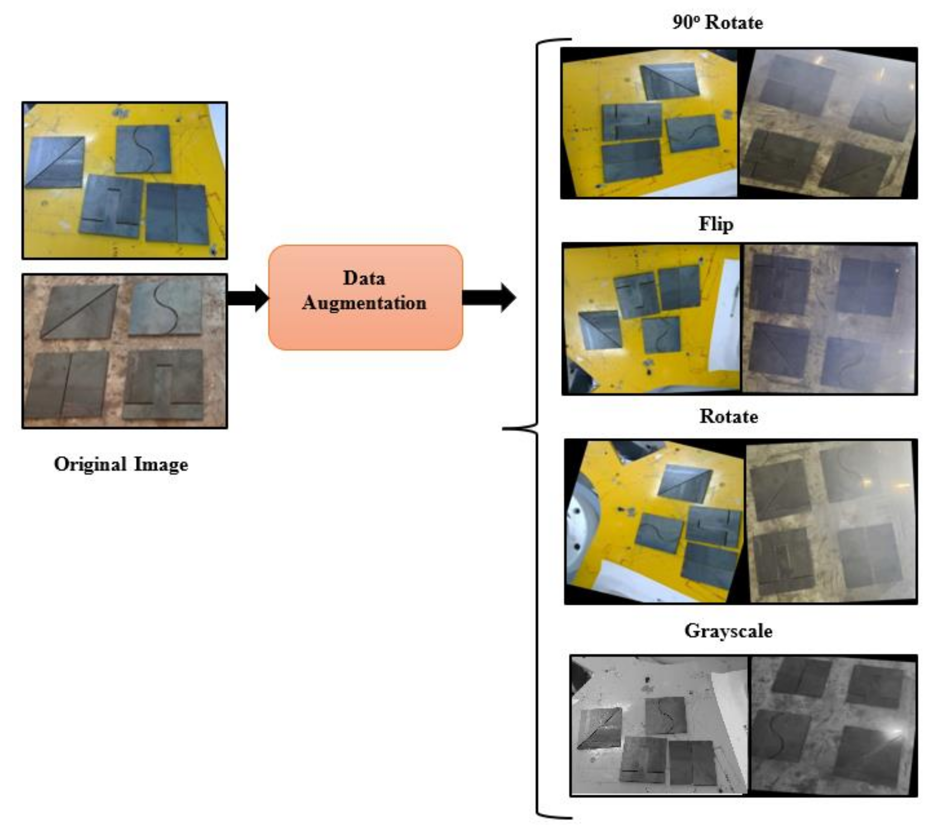
| Flip | Horizontal, Vertical |
| Clockwise | |
| Rotation | |
| Grayscale | 11% |
| Saturation | −30% to +30% |
| Contracting Path | Expansive Path | ||||
|---|---|---|---|---|---|
| Layer | Details | Output Size | Layer | Details | Output Size |
| Input | Weld Images | 572 × 572 × 3 | DWT UpSampling_1 | 2 × 2 × 1024 up sample of Conv5_2; Concat with Conv4_2 | 56 × 56 |
| Conv1_1 | 3 × 3 × 64; Linear ReLU | 570 × 570 | Conv6_1 | 3 × 3 × 512; Linear ReLU | 54 × 54 |
| Conv1_2 | 3 × 3 × 64; Linear ReLU | 570 × 570 | Conv6_2 | 3 × 3 × 512; Linear ReLU | 52 × 52 |
| Pool 1 | 2 × 2 Max Pool Stride 2 | 284 × 284 | DWT UpSampling_2 | 2 × 2 × 512 up sample of Conv6_2; Concat with Conv3_2 | 104 × 104 |
| Conv2_1 | 3 × 3 × 128; Linear ReLU | 284 × 284 | Conv7_1 | 3 × 3 × 256; Linear ReLU | 102 × 102 |
| Conv2_2 | 3 × 3 × 128; Linear ReLU | 282 × 282 | Conv7_2 | 3 × 3 × 256; Linear ReLU | 100 × 100 |
| Pool 2 | 2 × 2 Max Pool Stride 2 | 140 × 140 | DWT UpSampling_3 | 2 × 2 × 256 up sample of Conv7_2; Concat with Conv2_2 | 200 × 200 |
| Conv3_1 | 3 × 3 × 256; Linear ReLU | 138 × 138 | Conv8_1 | 3 × 3 × 128; Linear ReLU | 198 × 198 |
| Conv3_2 | 3 × 3 × 256; Linear ReLU | 136 × 136 | Conv8_2 | 3 × 3 × 128; Linear ReLU | 196 × 196 |
| Pool 3 | 2 × 2 Max Pool Stride 2 | 68 × 68 | DWT UpSampling_4 | 2 × 2 × 128 up sample of Conv1_2; Concat with Conv2_2 | 392 × 392 |
| Conv4_1 | 3 × 3 × 512; Linear ReLU | 66 × 66 | Conv9_1 | 3 × 3 × 64; Linear ReLU | 390 × 390 |
| Conv4_2 | 3 × 3 × 512; Linear ReLU | 64 × 64 | Conv9_2 | 3 × 3 × 64; Linear ReLU | 388 × 388 |
| Pool 4 | 2 × 2 Max Pool Stride 2 | 32 × 32 | Conv10 | 1 × 1 × 2; Linear ReLU | 388 × 388 |
| Conv5_1 | 3 × 3 × 1024; Linear ReLU | 30 × 30 | |||
| Conv5_2 | 3 × 3 × 1024; Linear ReLU | 28 × 28 | |||
| Layer | Details | Output Size |
|---|---|---|
| Input | Weld Images | 572 × 572 × 3 |
| Res2Net_1 | 3 Conv Layers 3 × 3 × 64 3 × 3 × 128; 3 × 3 × 256 | 566 × 566 |
| Res2Net_2 | 3 Conv Layers 3 × 3 × 64 3 × 3 × 128; 3 × 3 × 256 | 281 × 281 |
| Res2Net_3 | 3 Conv Layers 3 × 3 × 64 3 × 3 × 128; 3 × 3 × 256 | 134 × 134 |
| Attention Module_0 | 3 × 3 | 1024 × 1024 |
| Pixel Shuffle | Upscale factor = 2 | |
| Attention Module_1 | 3 × 3 | 256 × 256 |
| Upsampling_1 | 2 × 2; concat with Res2Net_2 | |
| Pixel Shuffle | Upscale factor = 2 | |
| Attention Module_2 | 3 × 3 | 192 × 192 |
| Upsampling_2 | 2 × 2; concat with Res2Net_1 | |
| Pixel Shuffle | Upscale factor = 2 | |
| Attention Module_3 | 3 × 3 | 112 × 112 |
| Upsampling_3 | 2 × 2; concat with Input layer | |
| Pixel Shuffle | Upscale factor = 2 | |
| Attention Module_4 | 3 × 3 | 44 × 44 |
| Conv_1 | 3 × 3 × 44 | 44 × 44 |
| Conv_2 | 3 × 3 × 44 | 28 × 28 |
| Layer | Details | Output Size |
|---|---|---|
| Conv_1 | 3 × 3 × 3; padding = 1 Leaky ReLU | 64 × 64 |
| Conv_2 | 3 × 3 × 64; padding = 1 Leaky ReLU; stride = 2 | 64 × 64 |
| Conv_3 | 3 × 3 × 64; padding = 1 Leaky ReLU | 128 × 128 |
| Conv_4 | 3 × 3 × 64; padding = 1 Leaky ReLU; stride = 2 | 128 × 128 |
| Conv_5 | 3 × 3 × 128; padding = 1 Leaky ReLU | 256 × 256 |
| Conv_6 | 3 × 3 × 256; padding = 1 Leaky ReLU; stride = 2 | 256 × 256 |
| Conv_7 | 3 × 3 × 256; padding = 1 Leaky ReLU | 512 × 512 |
| Conv_8 | 3 × 3 × 512; padding = 1 Leaky ReLU; stride = 2 | 512 × 512 |
| Conv_9 | 1 × 1 × 512 Leaky ReLU | 1024 × 1024 |
| Conv_10 | 1x 1 × 1024 Leaky ReLU | 1 × 1 |
| S. No | Environment | Values/Version |
|---|---|---|
| 1 | Operating System | Windows 11 |
| 2 | CPU | Intel(R) Core(TM) i7-9750H CPU @ 2.60 GHz 2.59 GHz |
| 3 | GPU | Tesla P100-PCIE-16 GB |
| 4 | RAM/ROM | 2666 MHz DDR4 16 GB |
| 5 | CUDA | 11.2 |
| 6 | cuDNN | 7.6.5 |
| 7 | IDE | Colab Pro Plus |
| 8 | Framework | pytorch |
| S. No | Parameter | Initial Value | Optimized Value (YOLOv4) | Optimized Value (YOLOv5) |
|---|---|---|---|---|
| 1 | Learning rate | 0.01 | 0.0121 | 0.0108 |
| 2 | Momentum constant | 0.93 | 0.937 | 0.98 |
| 3 | Weight decay | 0.0005 | 0.00039 | 0.00035 |
| 4 | Class loss | 0.5 | 1.09 | 1.42 |
| 5 | IoU_target | 0.2 | 0.2 | 0.2 |
| 6 | Anchor_target | 4 | 4.6 | 3.88 |
| 7 | Epochs | 50 | 200 | 200 |
| 8 | Dataset Split ratio | 60-20-20 | 60-20-20 | 60-20-20 |
| S. No | Parameter | Scaled YOLOv4 | YOLOv5 | YOLOv4 DarkNet | Faster RCNN | EfficientDet |
|---|---|---|---|---|---|---|
| 1 | Precision | 0.76 | 0.967 | 0.47 | 0.5 | 0.788 |
| 2 | Recall | 0.983 | 0.96 | 0.47 | 0.5 | 0.841 |
| 3 | mAP | 0.973 | 0.987 | 0.534 | 0.54 | 0.92 |
| 4 | F1 score | 0.85 | 0.96 | 0.54 | 0.5 | 0.813 |
| 5 | GIoU loss | 0.023 | 0.017 | 0.317 | 0.541 | 0.00089 |
| 6 | Object loss | 0.071 | 0.022 | 0.302 | 0.5084 | 0.133 |
| 7 | Class loss | 0.015 | 0.0046 | 0.34 | 0.212 | 0.169 |
| 8 | Training Time (h) | 0.901 | 0.710 | 0.534 | 1.5 | 0.583 |
| 9 | GPU memory | 5.51 GB | 1.89 GB | 1.70 GB | 6.7 GB | 1.5 GB |
| 10 | Total Loss | 0.109 | 0.0436 | 0.959 | 1.261 | 0.303 |
| S. No | Modules | Total Time (s) | Validation Accuracy (%) |
|---|---|---|---|
| 1 | Pre-processing + Scaled YOLOv4 + Contour detection | 4.387 | 81 |
| 2 | Pre-processing + Scaled YOLOv4 + GAN dehazing + Contour detection | 10.717 | 85 |
| 3 | Pre-processing + YOLOv5 + Contour detection | 0.0967 | 82 |
| 4 | Pre-processing + YOLOv5 + GAN dehazing + Contour detection | 6.426 | 89 |
| 5 | Pre-processing + YOLOv4 DarkNet + Contour detection | 20.828 | 70 |
| 6 | Pre-processing + YOLOv4 DarkNet + GAN dehazing + Contour detection | 27.158 | 76 |
| 7 | Pre-processing + Faster RCNN + Contour detection | 38.296 | 53 |
| 8 | Pre-processing + Faster RCNN + GAN dehazing + Contour detection | 44.626 | 61 |
| 9 | Pre-processing + EfficientDet + Contour detection | 0.855 | 89 |
| 10 | Pre-processing + EfficientDet + GAN dehazing + Contour detection | 7.185 | 93 |
| S.NO | Author | Methodology | Performance Metrics | Tracking Error |
|---|---|---|---|---|
| 1 | Yanbiao Zou et al., 2019 [11] | DCNN with VGGNet Weld seam searching with arc and splash noise | Inf time (356 images): 15.06 sec | Less than 1 mm |
| 2 | Chenhua Liu et al., 2022 [48] | Faster RCNN with different RPN networks | Validation accuracy: 86.45% Inference time: 25.02 ms | - |
| 3 | GuohongMa et al., 2021 [49] | CNN with AlexNet and VGG16 | Accuracy: AlexNet: 95.83%, VGG16: 89.17% Recall: 100% | - |
| 4 | Gwang-ho Yun et al., 2022 [50] | Contrast limited adaptive histogram equalization (CLAHE) and image denoising YOLO | Loss: 0.03415 mAP: 51.2% | - |
| 5 | Ran Li et al., 2021 [51] | Stacked denoising autoencoder (SDAE) for GMAW welding | Average error: 0.086 | - |
| 6 | Shao W et al., 2022 [52] | Periodic wide-field illumination | SNR: 35% | - |
| 7 | Present Method | DWT-GAN for dehazing And YOLOv5 | PSNR (GAN): 15.95 SSIM (GAN): 0.407 Validation Accuracy: 95% Total loss: 0.043 Inf time (212 images): 9.6 ms | Less than 0.3 mm |
Publisher’s Note: MDPI stays neutral with regard to jurisdictional claims in published maps and institutional affiliations. |
© 2022 by the authors. Licensee MDPI, Basel, Switzerland. This article is an open access article distributed under the terms and conditions of the Creative Commons Attribution (CC BY) license (https://creativecommons.org/licenses/by/4.0/).
Share and Cite
Singh, A.; Kalaichelvi, V.; DSouza, A.; Karthikeyan, R. GAN-Based Image Dehazing for Intelligent Weld Shape Classification and Tracing Using Deep Learning. Appl. Sci. 2022, 12, 6860. https://doi.org/10.3390/app12146860
Singh A, Kalaichelvi V, DSouza A, Karthikeyan R. GAN-Based Image Dehazing for Intelligent Weld Shape Classification and Tracing Using Deep Learning. Applied Sciences. 2022; 12(14):6860. https://doi.org/10.3390/app12146860
Chicago/Turabian StyleSingh, Abhilasha, Venkatesan Kalaichelvi, Ashlyn DSouza, and Ram Karthikeyan. 2022. "GAN-Based Image Dehazing for Intelligent Weld Shape Classification and Tracing Using Deep Learning" Applied Sciences 12, no. 14: 6860. https://doi.org/10.3390/app12146860
APA StyleSingh, A., Kalaichelvi, V., DSouza, A., & Karthikeyan, R. (2022). GAN-Based Image Dehazing for Intelligent Weld Shape Classification and Tracing Using Deep Learning. Applied Sciences, 12(14), 6860. https://doi.org/10.3390/app12146860