Article

GAN-Based Image Dehazing for Intelligent Weld Shape Classification and Tracing Using Deep Learning

1
Department of Electrical and Electronics Engineering, Birla Institute of Technology and Science Pilani, Dubai Campus, Dubai P.O. Box 345 055, United Arab Emirates
2
Department of Computer Science Engineering, Birla Institute of Technology and Science Pilani, Dubai Campus, Dubai P.O. Box 345 055, United Arab Emirates
3
Department of Mechanical Engineering, Birla Institute of Technology and Science Pilani, Dubai Campus, Dubai P.O. Box 345 055, United Arab Emirates
*
Author to whom correspondence should be addressed.
Appl. Sci. 2022, 12(14), 6860; https://doi.org/10.3390/app12146860
Submission received: 4 June 2022 / Revised: 24 June 2022 / Accepted: 28 June 2022 / Published: 6 July 2022
(This article belongs to the Special Issue Distributed Control for Robotics)

Abstract

:
Weld seam identification with industrial robots is a difficult task since it requires manual edge recognition and traditional image processing approaches, which take time. Furthermore, noises such as arc light, weld fumes, and different backgrounds have a significant impact on traditional weld seam identification. To solve these issues, deep learning-based object detection is used to distinguish distinct weld seam shapes in the presence of weld fumes, simulating real-world industrial welding settings. Genetic algorithm-based state-of-the-art object detection models such as Scaled YOLOv4 (You Only Look Once), YOLO DarkNet, and YOLOv5 are used in this work. To support actual welding, the aforementioned architecture is trained with 2286 real weld pieces made of mild steel and aluminum plates. To improve weld detection, the welding fumes are denoised using the generative adversarial network (GAN) and compared with dark channel prior (DCP) approach. Then, to discover the distinct weld seams, a contour detection method was applied, and an artificial neural network (ANN) was used to convert the pixel values into robot coordinates. Finally, distinct weld shape coordinates are provided to the TAL BRABO manipulator for tracing the shapes recognized using an eye-to-hand robotic camera setup. Peak signal-to-noise ratio, the structural similarity index, mean square error, and the naturalness image quality evaluator score are the dehazing metrics utilized for evaluation. For each test scenario, detection parameters such as precision, recall, mean average precision (mAP), loss, and inference speed values are compared. Weld shapes are recognized with 95% accuracy using YOLOv5 in both normal and post-fume removal settings. It was observed that the robot is able to trace the weld seam more precisely.

1. Introduction

Robotic welding is one of the most prominent industrial applications that performs repetitive tasks, and it has been utilized extensively in the automotive industry for decades. There is a significant demand for autonomous robotic welding [1] since the majority of joints in industry are irregular in shape. This has encouraged most businesses and researchers in robotic welding to use intelligent strategies to improve the quality and consistency of robotic welding. Furthermore, it is believed that robots can perform high-quality welding much more consistently than experienced workers. Additionally, robots can be programmed to work 24/7, maximizing productivity. There are numerous issues with weld seam identification, especially in the presence of industrial noise such as arc lights, flash, and welding fumes which are toxic to people, so robots are not capable of executing efficient path planning [2]. This research aims to remove weld fumes and identify weld shape using deep learning techniques to solve the aforementioned issues. Since deep learning models have better generalisation and regularisation ability, in this work, the generalisation ability of a YOLO-based detector is tested in different backgrounds with non-homogenous weld fumes. Weld seam detection can be divided into two categories: active vision and passive vision approaches [3]. The passive vision method using a 2D camera is used in this research, which decreases the cost and complexity of the experimental setup [4].
In the past few decades, research in robotic welding has been performed using conventional and deep learning methods for seam identification and tracking. Shah et al. have successfully detected autonomous weld seams and tested tracking of straight, zigzag, and half-moon shapes. The authors calculated accuracy in terms of position and distance error, which was calculated between the obtained output and actual weld seam path shape [5]. Li et al. used the optical triangulation method for detecting the position of weld seams using a structured light vision sensor [6]. Shao et al. performed calibration using a CCD camera and calculated the measurement error for arc-welding robots. The particle filter and Hough transform were used to detect the weld seam without any error between the welding position and the seam position. They were able to achieve a detection accuracy of 0.08 mm with 0.1 mm width for a narrow butt joint [7]. Lei et al. calculated the welding position using a vision sensor by implementing camera calibration and performed conventional image processing for circular weld seam detection. The image was found to dynamically change, which could be improved by machine learning techniques [8]. Yin et al. proposed two step calibration approaches, namely, camera calibration and light plane calibration for the autonomous detection of the weld seam and quality control. The authors were able to achieve a 0.2 mm tracking error [9]. Zou et al. proposed automatic weld seam detection using a deep convolutional neural network (CNN) to improve the tracking accuracy. The multi-correlation filter was implemented in real-time to detect the weld seam and position the weld torch, and the tracking error was found to be less than 1 mm for straight and curved weld seams [10]. Zhang et al. study the problem of domain generalization in object detection using sample reweighting method called region-aware proposal reweighting (RAPT). Extensive experiments were conducted on different datasets and various architectures [11].
According to the discussion above, there has been limited study on identifying weld seam shapes, which will be useful when the robot is unable to detect the welding area and can also be utilized as a first step in autonomous robotic welding. There are limited datasets for the welding process, particularly datasets with different shapes; hence, an attempt has been made to create datasets similar to the industrial process for weld shape detection. Additionally, major works on image denoising using GAN were tested on public datasets, and very few works were applied for custom datasets. So, GAN was used for weld fume removal in the current literature by applying image-to-image translation. Additionally, many authors used an expensive real-time experimental setup, including lasers and CCD cameras. As a result, a look-alike industrial welding setup has been demonstrated utilizing a simple 2D camera with two phases—dehazing using DW-GAN and a YOLO-based object detector—which is the major contribution of this work. Initially, mild steel and aluminium weld plates are recognized using several YOLO algorithms. If the image contains weld fumes, it is transferred to the dehazing step, where the fumes are removed using discrete wavelet-based GAN and dark channel prior methods. Further ablation studies and generalisation have been carried out for the deep learning models used in this work. After removing the fumes, the weld seam is retrieved using contour detection with binary thresholding, and its pixel coordinates are recorded as.csv files for subsequent processing. A neural network technique is applied to simplify the coordinate transition between weld contour locations and the robot in order to execute real-time robotic welding. For tracing the weld seam, the five DOF robot receives the robot coordinates obtained from the neural network model.
The following are the key goals of this paper:
  • Create a real-time weld dataset made up of actual weld plates with a variety of different weld shapes;
  • Remove weld fumes using the DW-GAN;
  • Train the dataset with genetic algorithm-based different YOLO approaches, such as Scaled YOLOv4, YOLOv5, and YOLOv4 DarkNet;
  • Determine the contours of various weld seam shapes using image processing;
  • Convert pixel coordinates to robot coordinates using a Backpropagation Neural Network model;
  • Perform real-time weld seam detection for tracing the weld seam shapes using a live 2D camera.
The paper is divided into five sections. Section 2 describes the GAN-based dehazing and object detection of the weld seam using different YOLO algorithms. This is followed by a discussion of the performance metrics used for weld seam detection in Section 3. The real-time experimentation results are discussed in Section 4, followed by the conclusion and future scope in Section 5.

2. Methods

In recent years, with advancements in computer vision and artificial intelligence, deep learning has gained popularity in industrial applications because it can handle larger data efficiently [12]. The methodology involved in deep learning-based weld seam detection is shown in Figure 1, and the detailed explanation is described in following sections. In Figure 1, images are captured using a Logitech c270 2D camera placed at an angle of 26° in eye-to-hand configuration. This camera is based on CMOS technology with a resolution of 720 p and 30 fps. If the images are clear without any fumes, then images are sent to the YOLO detector, but when it has fumes, these images are passed to the dehazing network where GAN is used to remove the nonhomogeneous weld fumes. Once the weld fumes are removed, images are sent to the YOLO model to detect the weld joints autonomously. These weld joints after classification are sent to contour detection block where binary thresholding is applied to extract the weld seam. These weld seam pixel coordinates were converted using an ANN model, as this is the simplest and easiest way for mapping input and output without complex calculations. The robot coordinates obtained were finally sent to robot for tracing the particular shape. In this work, the entire workspace is calibrated with backpropagation ANN model. This eliminates the need for camera calibration involving computation of transformation matrix. This matrix becomes complex when the number of robot joints increases. Hence, the ANN model is used for pixel-to-robot coordinate transformation for weld shape tracing.

2.1. Dataset Preparation

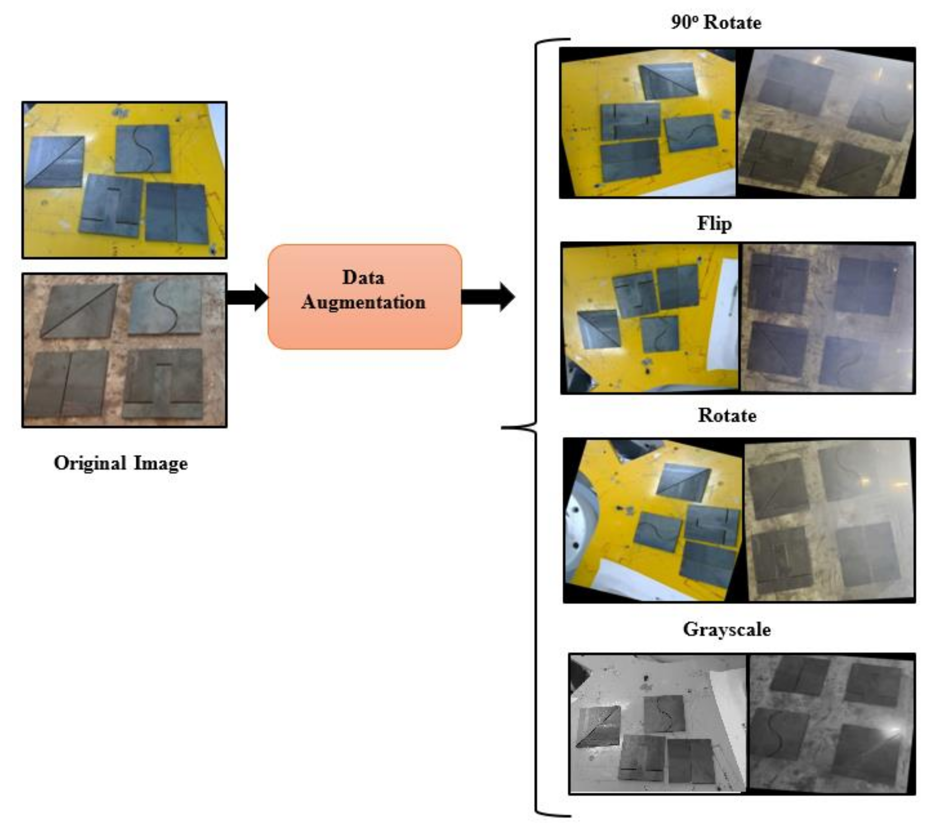
In any deep learning-based object detection, the initial step is data preparation and data cleaning. This is a very important step in any artificial intelligence technique because datasets contain duplicates and missing values which cannot be used to train deep learning models, as they may lead to larger errors in object detection [13]. The major steps in general include gathering the dataset, removing missing data and outliers, analysing the data, and finally converting it into a suitable format for the deep learning model for further processing [14]. In this work, actual weld plates were laser cut into eight different asymmetrical seam shapes to address the industrial welding process. The reason for choosing these shapes is that defected parts in industries are not symmetrical, so an attempt was made to prepare the dataset to identify the different shapes using a 2D camera with random positions at both the robot workspace and the welding table to create robust datasets. Furthermore, in order to increase the robustness of dataset and improve model training, data augmentation techniques were applied [15]. This was needed because datasets are prepared in limited conditions, but environmental conditions may vary in real-time scenarios, so different flips, rotations, saturation and grayscale were applied to the datasets. Additionally, weld fume images with arc light were also included to improve the weld seam detection. The major reason to choose a 2D camera is that they are easily available and the overall setup cost can be reduced. The main goal of this work was to train to the robot to detect and trace the weld plates anywhere in the workspace. About 2286 images were obtained which were manually labelled with the Roboflow image annotation tool. In data pre-processing, original data of 640 x 480 were resized to 416 x 416 pixels, making them suitable to train all the YOLO algorithms. The weld plate and augmentation specifications are tabulated in Table 1. The sample dataset of weld plates with different rotations is shown in Figure 2.

2.2. Dehazing Techniques for Weld Fume Removal

Hazy images, in general, affect numerous tasks such as tracking [16], satellite remote sensing [17], and object detection [18,19] due to color distortion, blurring and other visible quality degradation. Because of unequal haze distribution, many research papers have been published on deep learning-based dehazing approaches. Thus, to address these issues, discrete wavelet transform-based GAN (DW-GAN) [20] has been implemented to remove non-homogeneous weld fumes because dense welding fumes affect the path to be traced while welding. The GAN-based technique is compared with the conventional dark channel prior (DCP) method [21].

2.2.1. DW-GAN Architecture

In general, there are two major components in generative adversarial networks (GANs), namely, the generator and discriminator [22]. The generator is used for generating new examples, while the discriminator is used for classifying images as real or fake. The major applications where GANs have achieved great performance include synthesizing realistic images [23,24], image denoising and producing high-resolution images [25], single image dehazing [26], and image deraining [27]. DW-GAN architecture has two sub modules, namely, discrete wavelet and knowledge adaption. The discrete wavelet branch is used to learn direct mapping between ground truth and weld fume images, whereas the knowledge adaption branch uses prior knowledge from image classification for the current dehazing task. The architecture of DW-GAN is shown in Figure 3.
From the above diagram, the inputs were weld plates with fume images of size 1600 × 1200 × 3, which were resized to 572 × 572 × 3 for sending to the DW-GAN block, and the output was the fume-free image similar to the ground truth.

2.2.2. DWT Branch Using U-Net

In the first stage, the U-Net-based discrete wavelet transform (DWT) branch has a contracting path (encoder) and expansive path (decoder), as well as massive skip connections to preserve the texture details during the dehazing process to learn from both high-frequency and low-frequency components [20]. As the name suggest, the U-Net is ‘U-shaped’; the down-sampling module on the left performs convolution operation and the up-sampling module on the right performs transpose 2D convolution operation. The convolution operation with max pooling increases the depth of the image and reduces the size, while transposed convolution applies padding and upscales the image, creating a clean image pixel by pixel, and thereby removing the weld fumes. The detailed U-Net DWT architecture for weld images is shown in Table 2.
Here, input features are converted into low-frequency and high-frequency components where low frequency components are added to the convolution and high-frequency components are added to the DWT up-sampling module. In 2D DWT, four filters are used, i.e., a low-pass filter and high-pass filters with stride 2 convolution operation. Using convolution operation with these filters, images or feature maps are decomposed into four sub bands, i.e., x L L , x L H , x H L , , and x H H .The equation for x L L is given by:
x L L = x 2 i 1 , 2 j 1 + x 2 i 1 , 2 j + x 2 i , 2 j 1 + x 2 i , 2 j
The equations of x L H ,   x H L ,   x H H are same as x L L , which is helpful in retaining the hazy images and thereby learning spatial and frequency information.

2.2.3. Knowledge Adaption Branch Using ImageNet and Res2Net

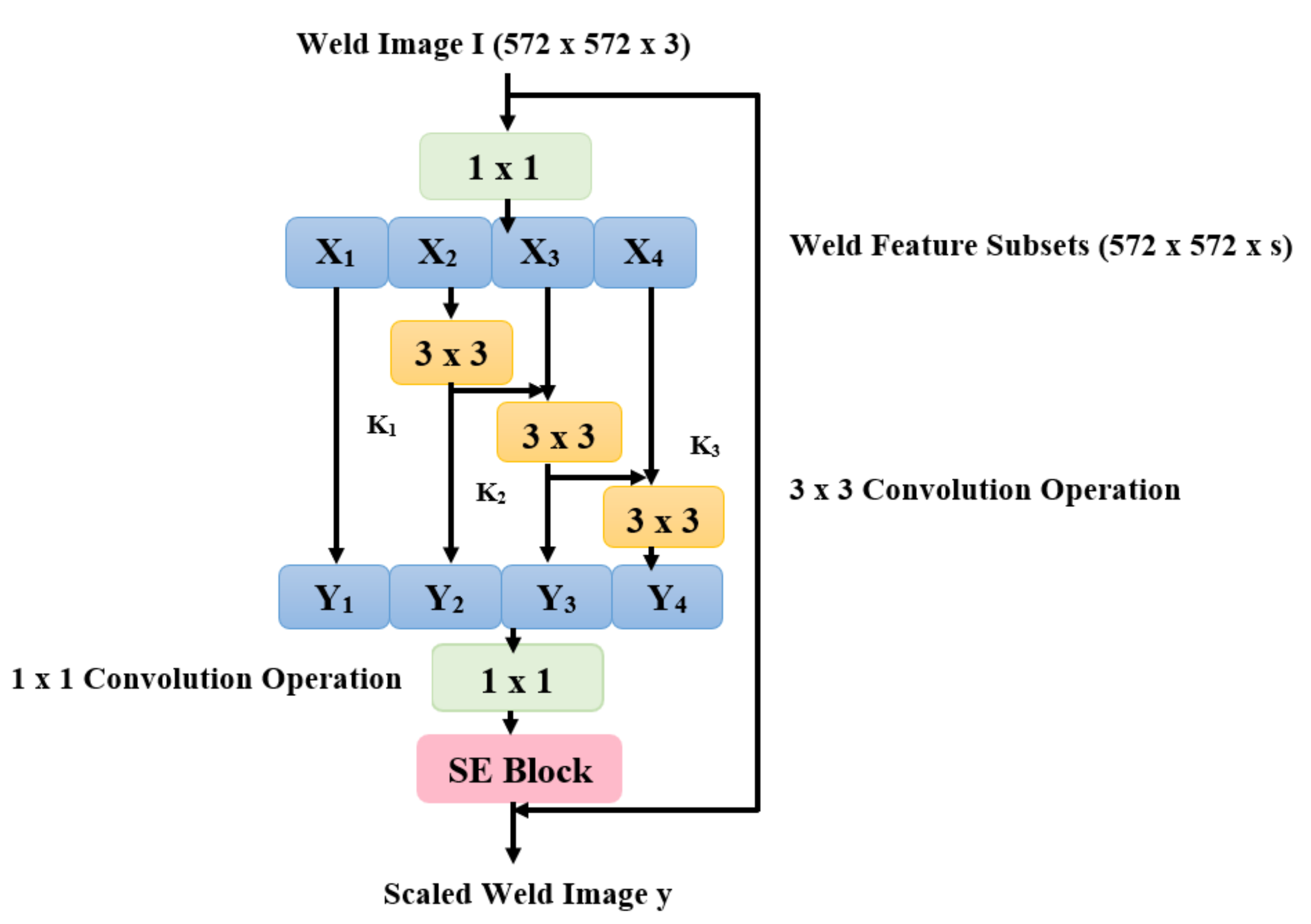
In second stage, the knowledge adaptation branch uses the ImageNet [28] pre-trained Res2Net [29] as the backbone of the encoder, making DW-GAN more robust with better generalization ability. The Res2Net architecture with the squeeze and excitation networks (SE) is shown in Figure 4.
In Res2Net architecture, after 1 × 1 convolution features of Image I, X i is evenly split into s subsets with i    1 , 2 , . . , s . To reduce the number of parameters, 3 × 3 group filters are omitted for X 1 and smaller filters are used for X i 1 . The output Y i can be written as:
Y i = X i ,                                   i = 1 K i X i ,                 i = 2 K i ( X i + Y i 1 ,   2 < i s  
Furthermore, we concatenate all the subset features into single ones by using 1 × 1 convolution, and at the end the SE network is added to adaptively recalibrate the channel-wise responses y . The detailed knowledge adaption architecture used is described in Table 3.
In addition to Res2Net, attention modules are added to detect dynamic hazy patterns, whereas pixel shuffle layers are added before the attention module to upscale the image, thereby reducing the computational cost. Finally, a simple 7 × 7 convolution layer with tanh activation layer is added for fusing the combined features from the above two stages to produce weld-fume-free images.

Discriminator

The discriminator uses real data as positive examples and dehazed images as negative examples, and image-to-image translation takes place during training. The discriminator tries to identify between dehazed images and ground truth. It then penalises if it misclassifies. The detailed architecture for the discriminator is described in Table 4.
During the entire training period, total loss is nothing but the sum of smooth loss, perpetual loss, multi-scale structural similarity index measure (MS-SSIM) loss, and adversarial loss.
L t o t a l = L s m o o t h + α L M S S S I M + β L p e r p e c t u a l + γ L a d v
where α = 0.2, β = 0.001, and γ = 0.005. The details of loss functions are referenced in [30]. The two most important metrics are used to measure the performance of GAN output (dehazed image), namely, peak signal-to-noise ratio (PSNR) and SSIM [30]. The equations of PSNR and SSIM are as follows:
P S N R = 10 log 10 ( m a x I ) 2 M S E
M S E = 1 m n i = 0 m 1 j = 0 n 1 I i , j K i , j 2  
The SSIM [31] measures image similarity by calculating luminance, contrast, and structure. The luminance function, contrast function, and structure function can be expressed as follows:
l x , y = 2 μ x μ y + c 1 μ x 2 + μ y 2 + c 1
c x , y = 2 σ x σ y + c 2 σ x 2 + σ y 2 + c 2
s x , y = σ x y + c 3 σ x y + c 3
Using the above three equations, SSIM is calculated as follows:
S S I M x , y = l x , y α c x , y β s x , y γ
where α = β = γ = 1 ; c 1 = k 1 L 2 ; c 2 = k 2 L 2 ; k 1 = 0.01 ; and k 2 = 0.03 .
The GAN network was trained with 674 samples using Tesla P-100 GPU cards with pytorch as a deep learning framework. The Adam optimizer was used with a learning rate of 1 × 10⁻⁴, and it was trained for 3000 epochs. The GAN performance was compared with the DCP method. The dehazed images were sent to the deep learning model for classification.

2.3. Theoretical Background of YOLO Architecture

You Only Look Once (YOLO) is a popular single-stage object-detection algorithm that uses a single neural network to perform both the classification and prediction of bounding boxes. The main working of YOLO is that the images are split into S × S square grids where each cell will predict B bounding boxes of weld shapes with a confidence score for each box. YOLO finally predicts bounding boxes with x coordinates, y coordinates, box width w , box height h , and confidence c . The confidence score varies between 0 to 1 where 0 means no object exists in that cell and 1 means weld shapes are present in that cell. The coordinates x ,   y are the centroid of the predicted bounding box, and the width and height are fractions relative to the entire image size. The confidence is calculated based on the intersection over union (IOU), which is nothing but the area of overlap between the predicted and ground truth boxes divided by the area of the union [32,33]. In this work, different versions of YOLO algorithms such as YOLOv4 DarkNet, Scaled YOLOv4 and YOLOv5 are used, and their performances are compared.

2.3.1. YOLOv4 Architecture

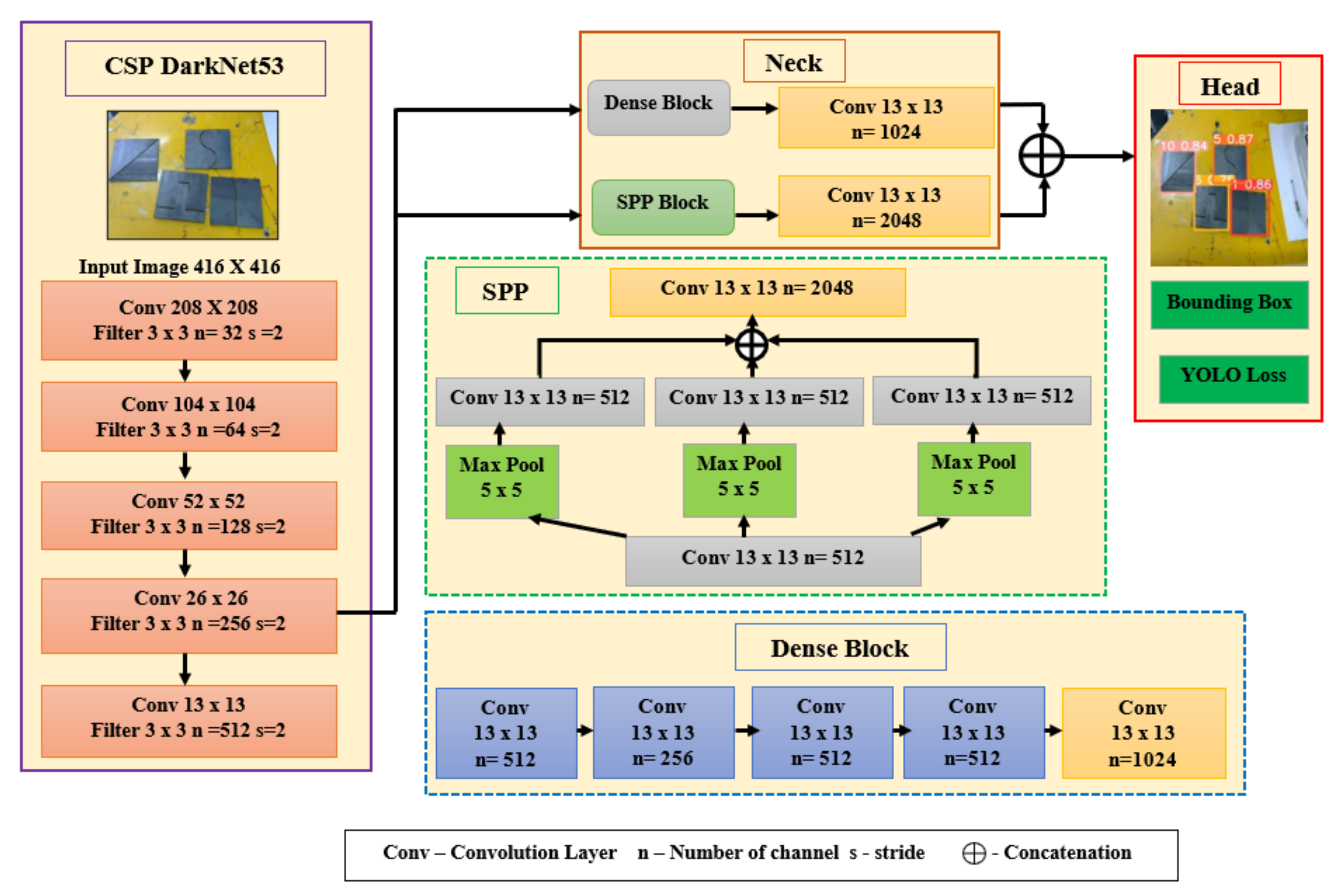
YOLOv4 DarkNet with Scaled YOLOv4 is the one of the accurate neural network models produced in recent times for single-stage object detection. Its architecture is made up of three parent blocks, namely, backbone, neck and head, as shown in Figure 5, with 334 layers. This architecture uses cross-stage partialized (CSP), in which feature maps of the base layer are partitioned into two sections and finally merged into the transition layer [34,35]. This initiates the gradient flow through different network paths, thereby reducing the amount of computation and inference speed, as well as accuracy.
The input image is fed into the backbone layer which is responsible for convolutional down sampling to extract the features. In this work, CSPDarknet53 is used as the backbone for object detection, which has 53 convolutional layers with high accuracy [36]. The dense block contains multiple convolution layers starting from 13 × 13 × 512 as the input layer X o and finally 13 × 13 × 1024 as the output transition layer. The neck layer serves as the extra layer between the backbone and the head for in-depth prediction [37]. In Scaled YOLOv4, PAN network and modified SPP (spatial pyramid pooling) constitute the neck layer. The SPP retains the output of the spatial dimension and removes fixed size constraints. The path aggregation network (PANNet) is added for the aggregation of features and image segmentation, which preserves the spatial information present in the images [38]. Here, three anchors—[12, 16, 19, 36, 40, 28], [36, 75, 76, 55, 72, 146] and [142, 110, 192, 243, 459, 401]—were used and each bounding box predicted the offset from the top corner of each image ( c x , c y ), as well as B w width, B h height and probability (confidence) score c . The governing equations for bounding boxes are as follows:
B o u n d i n g   B o x   c o o r d i n a t e s , B x = 2   σ t x 0.5 + c x
B y = 2 σ t y 0.5 + c y
B o u n d i n g   B o x   w i d t h , B w = 2 σ t w 2 P w
B o u n d i n g   B o x   h e i g h t , B h = 2 σ t h 2 P h
σ t = p r c o n t a i n i n g   o b j e c t   x   I o U p r e d i c t e d   b o x , G r o u n d   t r u t h   b o x
C o n f i d e n c e   S c o r e =   c =   pr object     IoU
The YOLOv4 network uses cross minibatch normalization so that it can work on any GPU. Furthermore, there are many regularisation techniques in the literature, but DropBlock regularisation was used in this work where certain parts of the image were hidden, and the network was forced to learn the other features rather than relying upon important features [39,40]. There are two main parameters, namely, block size and γ, which determine the number of units to be dropped. The larger the block size the more features are masked, which makes stronger regularisation. The equation for γ is shown below:
γ = 1 k e e p _ p r o b b l o c k _ s i z e 2   f e a t _ s i z e 2 f e a t _ s i z e b l o c k _ s i z e + 1 2
where k e e p _ p r o b is the threshold probability value (values below this threshold will be masked) and f e a t _ s i z e is the size of the feature map.

2.3.2. YOLOv5 Architecture

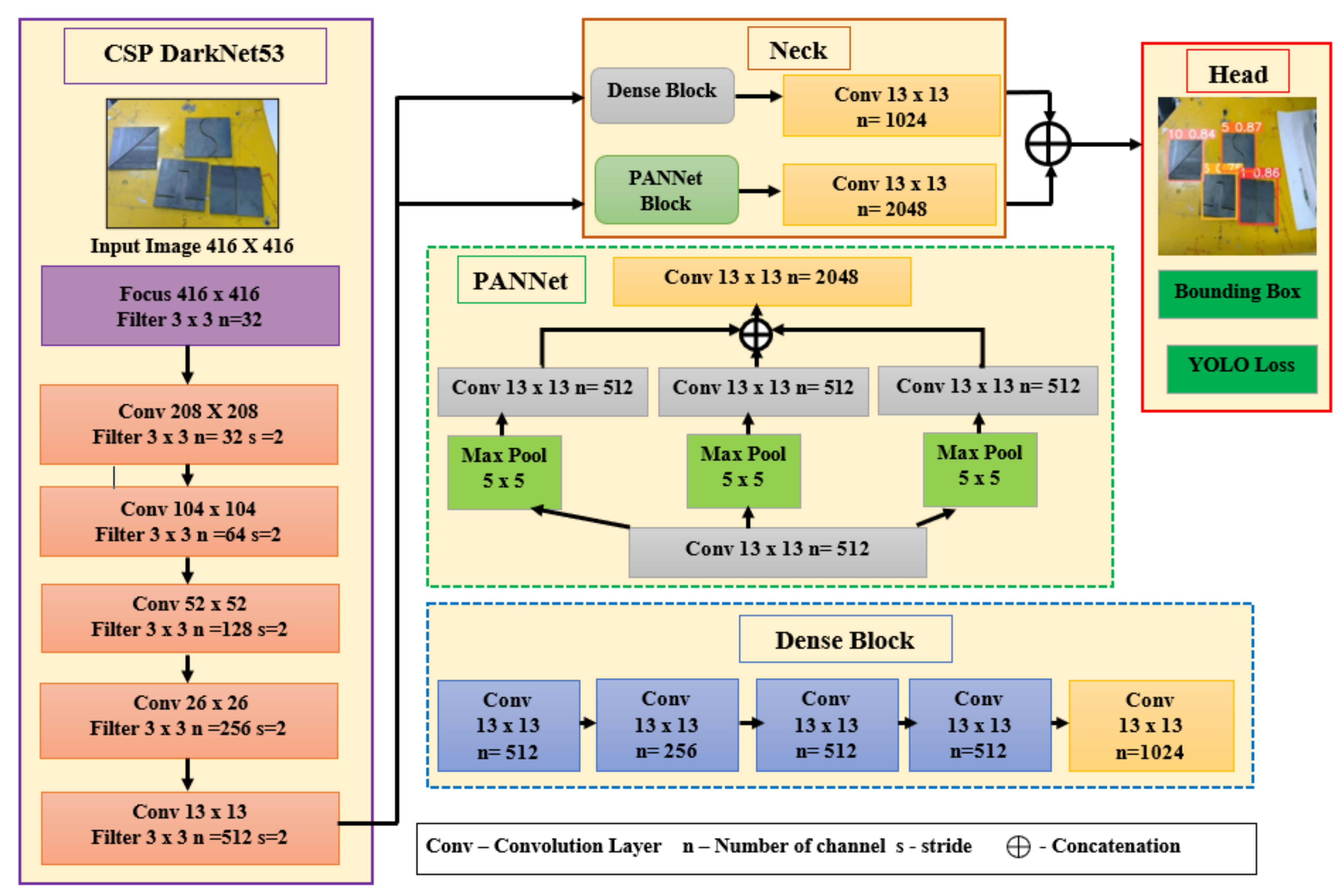
YOLOv5 is an improved deep learning model and is more efficient than YOLOv4 and Scaled YOLOv4. It uses three stages—model backbone, model neck and model head [41]—with a total of 283 layers. The major difference between YOLOv4 and YOLOv5 is that YOLOv5 uses focus layer and PANNet. The focus layer is introduced to reduce the number of layers and reduce its parameters, thereby reducing CUDA memory. This increases the training speed while minimally impacting mean average precision (mAP). The CSPDarkNet53 is used as the backbone layer which extracts the important features from the given input image, improving the processing time. Next, PANNet is used with the neck to generate feature pyramids so that the models have better generalization and scaling ability [42]. It also helps to identify the different sizes and scales for the same object. Finally, the head is same as the YOLOv3 and v4 versions, and is used to perform the detection with vectors of class probabilities, objectness scores, and bounding boxes [43]. The YOLOv5 architecture is shown in Figure 6. The final output of the abovementioned deep learning models is a vector of 13 × 13 × (5*3 + 8) predictors for each image, which is 13 × 13 × 23. In this work, the genetic algorithm (GA) is used to find the best parameters for training both YOLOv4 and YOLOv5 and, using these parameters, the model is trained for class and bounding box prediction. The parameters of the GA algorithm used for this work are discussed in Section 4.3. Finally, the performance of the YOLO algorithm is analysed with EfficientDet and Faster RCNN, which is a two-stage detector. The architecture used for comparison was Inceptionv2. The model was trained for 200 epochs with a batch size of 16 and a 416 × 416 image size. The learning rate was chosen as 1e-4 with the SGD optimiser. The pretrained model weights based on COCO datasets were used so that the model could be trained with smaller batches of custom datasets. Next, L2 regularisation was used in faster RCNN because it penalises the cost function based on the squared mean of the coefficients so that the model does not overfit. The cost function is the sum of the squared error with the L2 regularisation term and the equation is as follows:
c o s t = i = 0 n y i j = 0 M x i j w j 2 + j = 0 M w j 2
where x i j is the input to the network; y i is the output of the network; and w j is the weight of the network.
Additionally, a genetic algorithm with 100 generations, 0.9 mutation probability and a sigma value of 0.2 was implemented to find the optimal training hyperparameters of YOLOv4 and YOLOv5. This further improved the weld shape classification.
The pseudocode for overall weld seam detection using different YOLO algorithms is given as follows Algorithm 1:
Algorithm 1 Pseudocode of Weld Seam Detection using YOLO Algorithms
Begin
Input: weld images I_weld, Bounding box coordinates x, y width Bw, height Bh
Output: Class probabilities Pc and Predicted Bounding box coordinates
Data partition: I_weld = I_train (60%)+I_test (20%)+I_validation (20%)
Initialize no of epochs N = 200
batch_size = 16
Resize the image to 416 × 416
Generation = 100
Mutation_probability = 0.9
Sigma = 0.2
for i = 1 to generation
for j = 1 to batch_size
Load pretrained weights w
Load yolo configuration files
Run GA to obtain best hyperparameter values
end for
end for
Training phase:
for i = 1 to N
Load optimized weights and biases
Load optimized yolo training parameters from GA
Perform training on I_train
end for
save checkpoint weights.ckpt
Testingphase:
for each videoframe do
I_test = capture(videoframe)
predict y = f(Pc, Bw, Bh, Bx, By)
No of predictions = 13 × 13 × (5*3 + c)
Display class c and Pc
end for
end

2.4. Contour Detection for the Extraction of Weld Seams

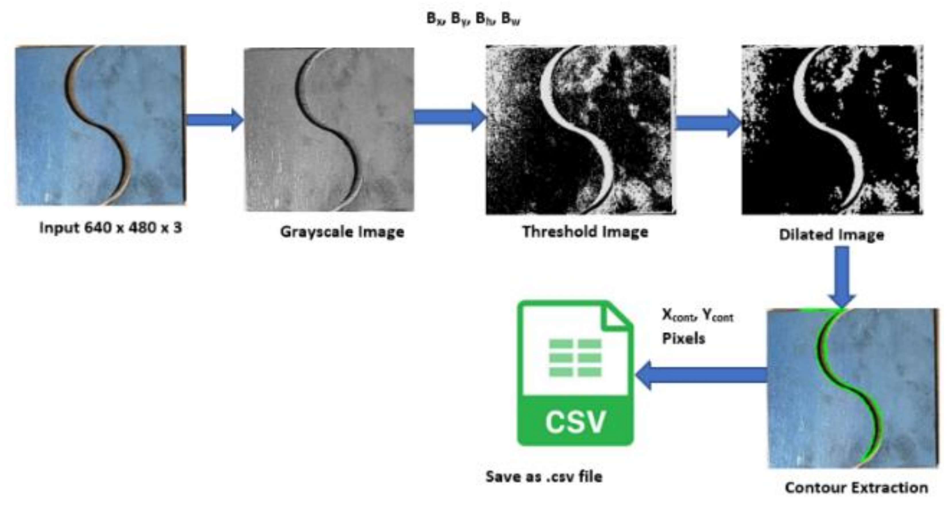
In image processing, contour detection helps in finding the same intensity points along the boundary of any object in the image. This is helpful in object detection and recognition applications. In this work, ten different weld seam shapes needed to be identified for the robot to trace the shapes accordingly. Hence, contour detection was implemented using OpenCV to identify the contours present in the weld plates. To improve the accuracy of detection, the weld image obtained from the live camera feed was converted into a grayscale image which was further cropped based on the predicted bounding box coordinates. To obtain better accuracy, the image was thresholded and then it was eroded and dilated [44]. Furthermore, contours were sorted, the largest contours present in the image were taken, and the contour lines were drawn around the weld seam, indicating boundaries of the same intensities or pixel values. Finally, all the contours for the particular shape were saved in csv format to convert the contour pixels into robot coordinates for robotic welding. The overall contour detection process flow diagram for shape number 5 is shown in Figure 7.
The pseudocode for contour detection is as follows Algorithm 2:
Algorithm 2 Pseudocode of Contour Extraction of Weld Seam
Begin
Input:Image 640 × 480 × 3; I = f (u, v,3)
Output:Contour Points C = (xcont, ycont)
fori = 1 to n
Read test weld image or live camera image I = f(u, v,3)
Extract the individual channels from RGB image,
R = I (:, :,1);
G = I (:, :,2);
B = I (:, :,3);
Grayscale Conversion, grayImage = (R+G+B)/3
Perform Inverted Binary Image thresholding, set T = 100
iff (x, y) > T
then f (x, y) = 0
else
f (x, y) = 255
end if
Perform erosion and dilation
Find contours using C = cv2.findContours()
Draw contours using C pixel points
end for
Save contour points C to .csv
end

3. Evaluation of Weld Seam Detection

The performance of the model is verified using four main object detection metrics. Specifically, the Precision, Recall, mAP, and F1 Score were adopted for evaluation in this study [45], and the equations are shown in the following Equations (18)–(22). The higher the value of Precision, mAP and F1 Score, the better the detection result of the weld seam shapes.
P r e c i s i o n = T P T P + F P   100 %
R e c a l l = T P T P + F N   100 %
m A P = c = 1 C A v e r a g e   P r e c i s i o n c C
F 1   S c o r e = 2     P r e c i s i o n     R e c a l l P r e c i s i o n + R e c a l l
I o U = A r e a   o f   o v e r l a p A r e a   o f   u n i o n
where C = number of classes;
T P = true positive; detected bounding box overlaps with ground truth boxes;
F P = false positive; detected bounding boxes away from ground truth boxes;
T N = true negative; does not predict bounding boxes in unwanted region;
F N = false negative; fail to predict bounding boxes with ground truth boxes.
Further inference speed and memory utilisation for different YOLO algorithms were analysed and compared with the detection performance.

4. Results and Discussion

4.1. Experimental Setup for Real-Time Weld Seam Tracing

The deep learning-based welding robotic system was implemented in a five DOF TAL BRABO manipulator. This manipulator has five joints named x ,   y ,   z ,   u and v . The x , y , and z joints are the three main joints and u and v are the wrist joints in this robot. Since there is no yaw motion in this robot, it is considered a five DOF robotic manipulator. The main reason to implement this work on this robot is that this robot has different kinematic and dynamic configurations, and no such experimental study has been tested on this robot. Hence, this work was carried out on a TAL BRABO robot. Secondly, there is very limited work on deep learning-based weld shape detection and tracing. The communication to TAL BRABO joints takes place through ActiveX commands written in MATLAB which communicates with the robot via a Trio motion controller. This controller is placed inside the programmable logic circuit (PLC) station from which robot is switched on. The vision system used in this paper was eye-to-hand configuration; a single 2D web camera was used, tilted at an angle of 26° to view the robot workspace where the weld plate was placed. Additionally, the camera was placed at an angle of approximately 32 degrees away from the robot base axis in order to make the problem a challenging one. Apart from the rotation and the translation of the camera into world coordinates, there was additional rotation from the axis of the robot base. This complex kinematic analysis was solved by using a neural network to convert pixel coordinates into world coordinates, as discussed in Section 4.5. The structure of the entire experimental setup is shown in Figure 8.

4.2. Weld Fume Removal Using GAN

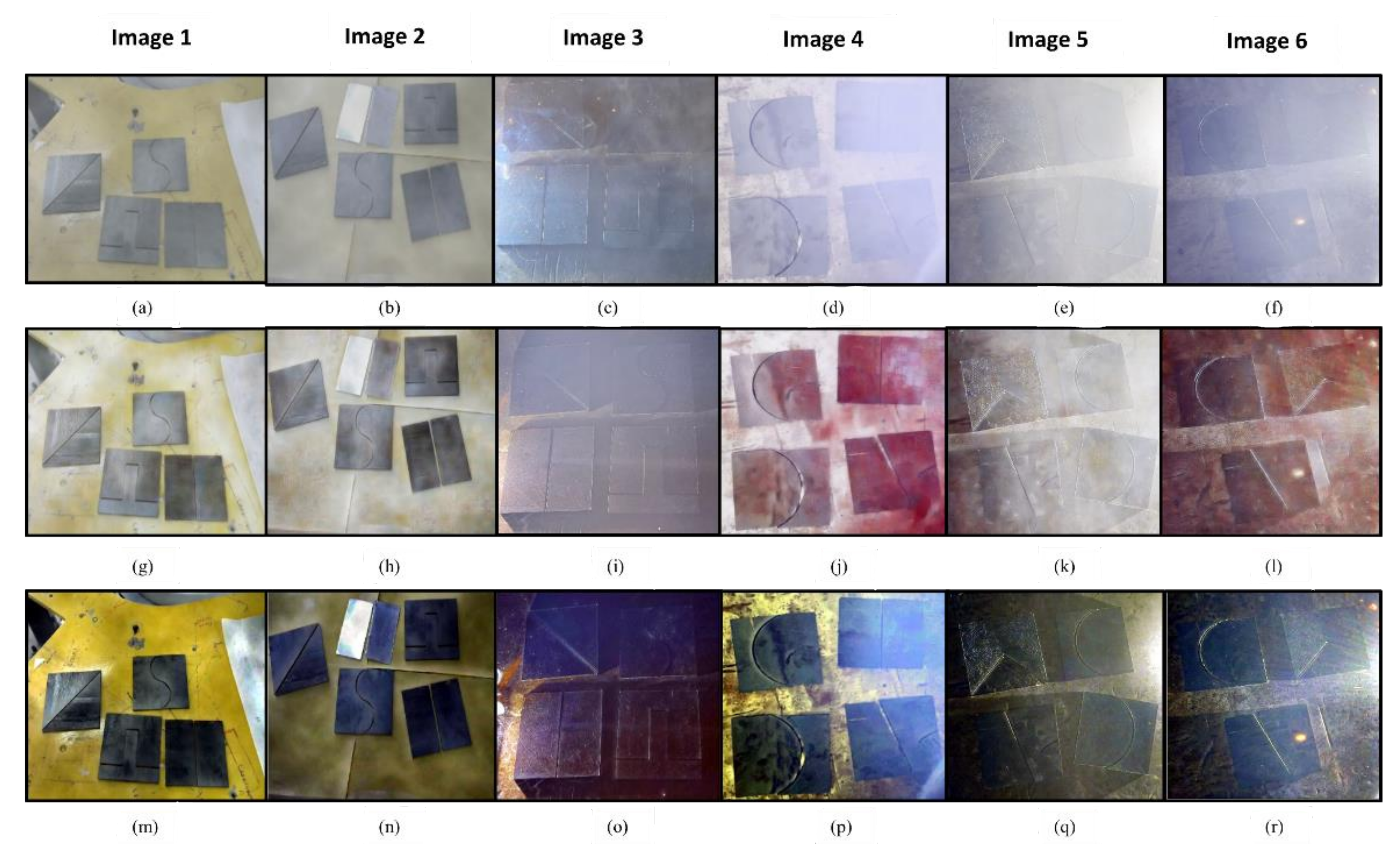
In this section, real-time experiments related to weld fume removal are discussed. The datasets used for analysing the dehazing performance included nonhomogeneous fumes present over the plates. Additionally, to make the detection robust, plates were placed in different backgrounds to prepare the datasets. In this paper, DW-GAN was used for fume removal and was trained for 3000 epochs with an image size of 1600 × 1200 pixels. The learning rate was chosen as 1e-4. The ground truth image used is shown in Figure 9a–f. The dehaze results for GAN are shown in Figure 9g–l, and for DCP they are shown in Figure 9m–r. The inference speed for DW-GAN was found to be 6.33 s, and for the DCP method it took 20.14 s for a single image.
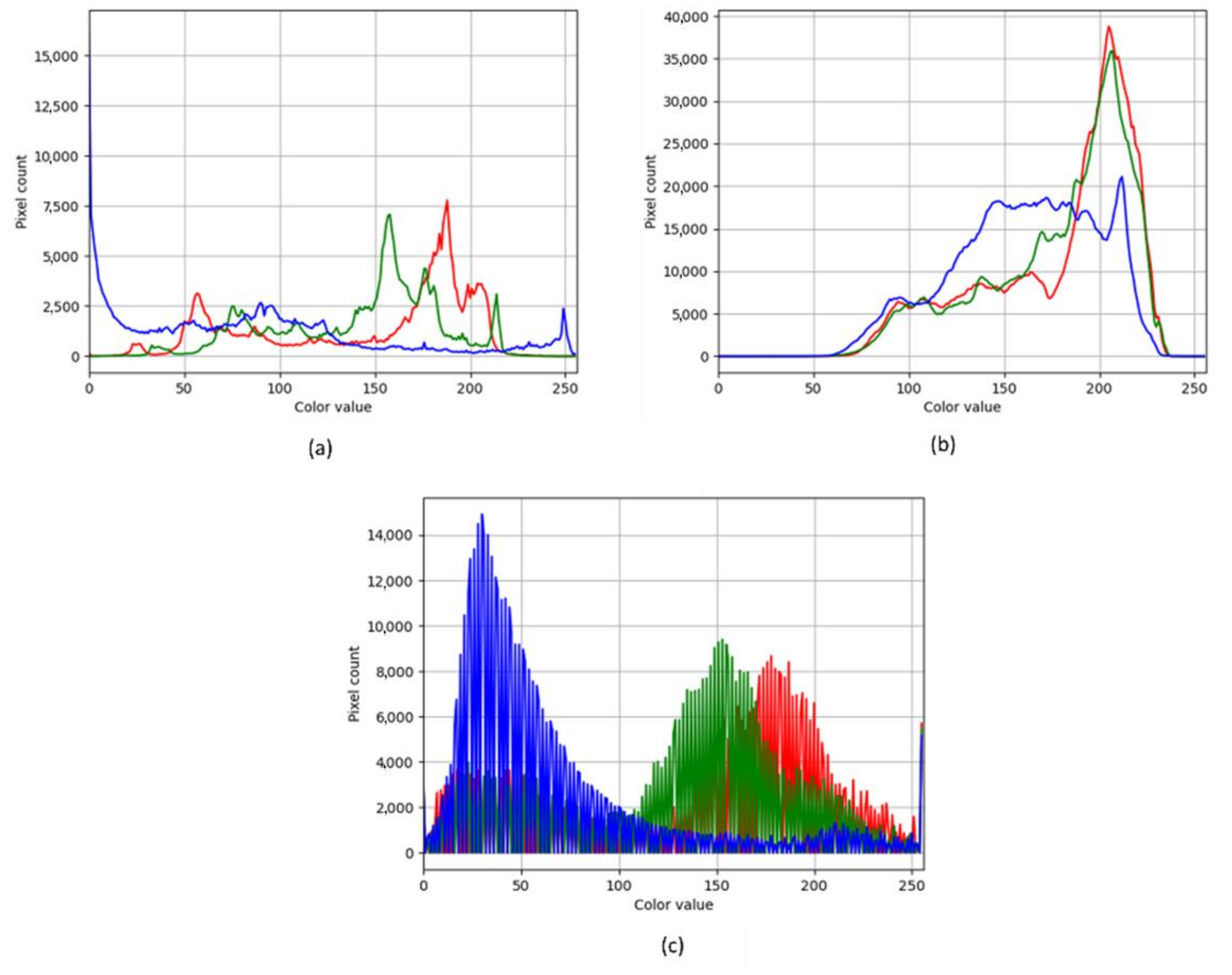
The image histogram calculated from image 1 is shown in Figure 10a–c to compare the variations in pixels between ground truth and dehazed images using the GAN and DCP methods.
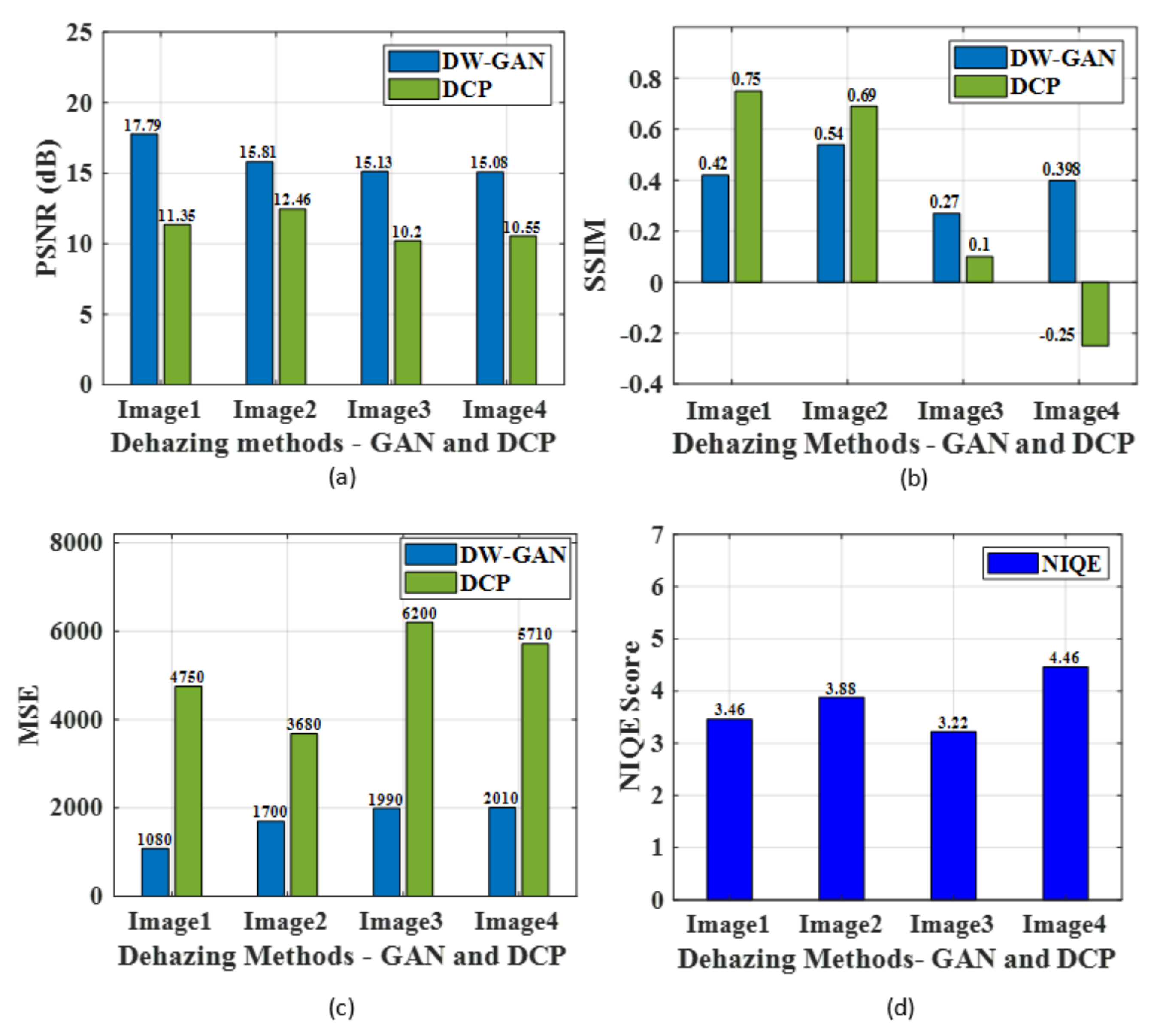
The RGB variations in ground truth and dehazed image are plotted and, from the graph, it can be inferred that pixel values were better for the GAN images, which were similar to ground truth. Furthermore, to analyse the dehazing performance, PSNR, SSIM, MSE and NIQE scores for image 1 to image 4 are analysed and plotted in Figure 11a–d, respectively.
From the plot, it can be seen that PSNR for GAN was high for all four images, which shows that image quality was better than DCP-based weld fume removal. The average PSNR of GAN was obtained as 15.95 dB, which was higher than DCP. Similarly, SSIM value for GAN-based weld fume removal was high, with an average value of 0.407, which implies better quality than the DCP method. Additionally, it was noted that the mean square error was less for the GAN-based dehazing method with a value of 1.69e+3. Hence, it can be concluded that the GAN method was more effective at removing the weld fumes than the conventional DCP method, and also preserved the image quality. Furthermore, the dehazed images were sent for training along with the other images for weld seam detection.

4.3. Training Phase of Weld Seam Detection using YOLO Algorithms

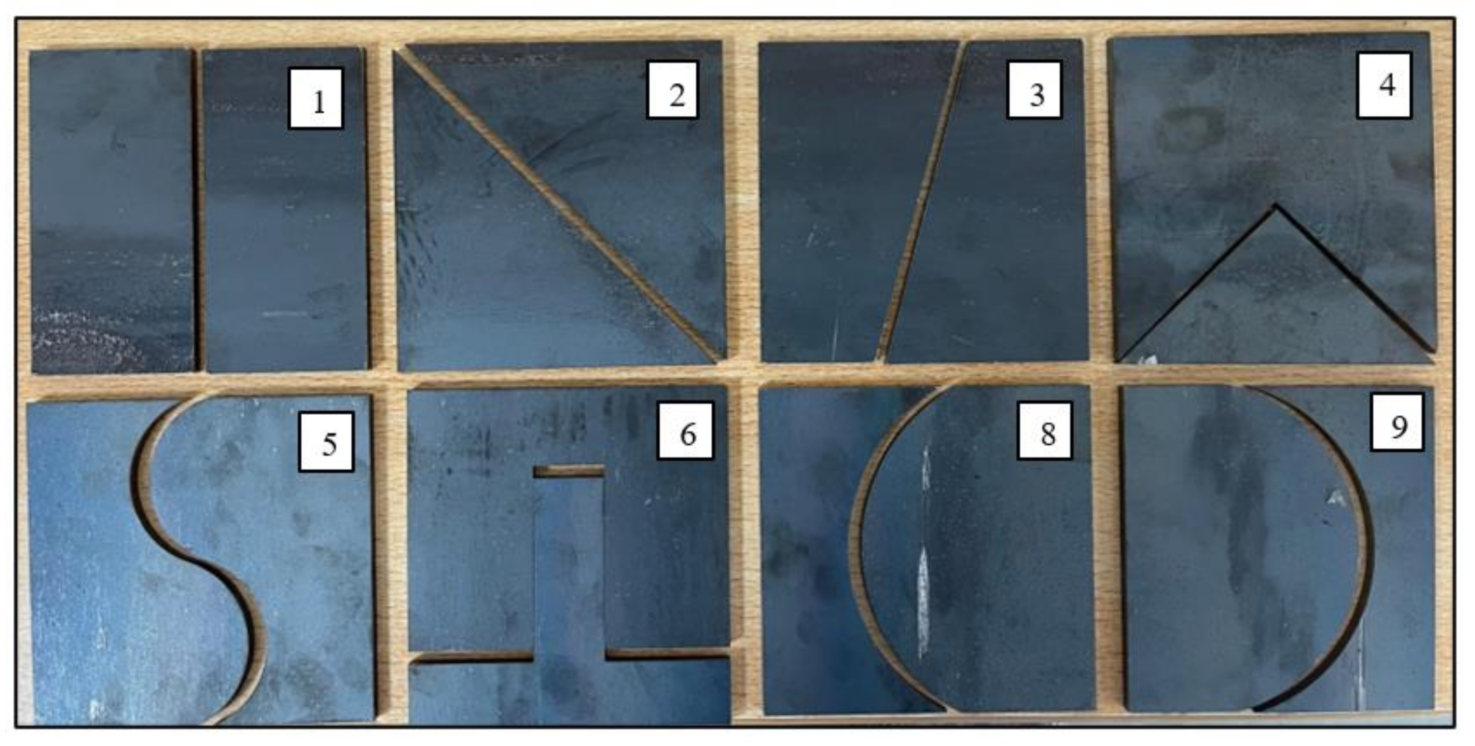
The weld datasets of the different shapes, as shown in Figure 12, were trained using different versions of the YOLO algorithm with GA-evolved parameters. The total dataset comprised 2286 samples, of which YOLO was trained with 1866 training weld images using pretrained weights of CSPDarknet53 to avoid training from scratch and save training time. The input size was 640 × 480 which was resized to 416 × 416, as well as augmented to increase the dataset. The model was trained on Tesla P-100 with the 11.2 CUDA version. The main purpose of the YOLO training was to minimize the loss function. The optimization equation for YOLO is as follows:
J = min   c o o r d i = 0 s 2 j = 0 B 1 i j o b j x i x i ^ 2 + y i y i ^ 2   + c o o r d i = 0 s 2 j = 0 B 1 i j o b j w i w i ^ 2 + h i h i ^ 2 + i = 0 s 2 j = 0 B 1 i j o b j c i c i ^ 2 + n o b j i = 0 s 2 j = 0 B 1 i j n o b j c i c i ^ 2   + i = 0 s 2   1 i j o b j c c l a s s e s p i c p i ^ c 2
where ( x i , y i ) represents the centroid of the bounding box; ( w i , h i ) denotes the width and height of the bounding box; c i represents the confidence score;   c o o r d and n o b j are constants which describe the important term to account for; p i c is the classification loss; 1 i j o b j is 1 if the object appears in the cell, or else 0; and 1 i j n o b j is 0 if the object appears in the cell, or else 1. Next, the GA was used to optimise the training parameters where the number of generations was chosen as 100. The highest fitness was selected for mutation based on a normal distribution of 20%. The confident score was calculated based on the weighted intersection of union (IoU) and the probability of objects present within the grids. The overall batch size was chosen as 16, which was made to run for 200 epochs with an SGD optimiser. The learning rate was kept constant with the value of 0.01. Hence, the genetic algorithm ran for 100 generations, producing efficient optimal values. The hardware and deep learning parameters are listed in Table 5. The initial and optimised training parameters of YOLO were manually adjusted, and are listed in Table 6.
The performance metrics for Scaled YOLOv4, YOLOv5, Faster RCNN, EfficientDet and YOLOv4 DarkNet are listed in Table 7, which was obtained after training the network with optimized training parameters. The performance of the single-stage detector was compared with the two-stage detector Faster RCNN with the Inception v2 model.
It can be inferred from the above table that the Precision and Recall values of YOLOv5 were better than Scaled YOLOv4, YOLOv4 DarkNet and Faster RCNN, with the values of 96.7% and 96%, respectively. However, the performance of YOLOv5 and EfficientDet was similar, and the model was fast and accurate. Additionally, the total loss of YOLOv5 was comparatively smaller with the value of 0.0436, and it was high for Faster RCNN with the value of 1.261. This shows that, for the weld dataset, YOLOv5 performed better than the other algorithms.

4.4. Testing Phase of Weld Seam Detection Using YOLO Algorithms

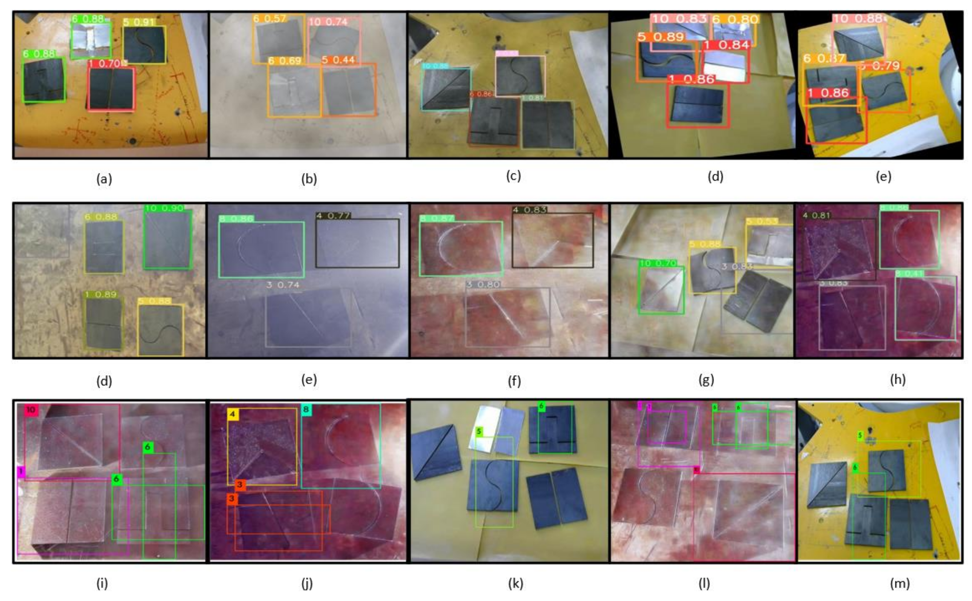
To test the effectiveness of the trained model, it was validated with 208 images and the generalisation ability of the model was tested on 212 test images with GA optimal parameters. Additionally, testing was performed by capturing the weld plates from the live camera kept in eye-to-hand configuration to show the robustness of detection. Furthermore, the inference speed of YOLOv5 was just 0.096 for the 212 test images, whereas DarkNet took 20.73 s, which was comparatively higher. The faster algorithms could be useful in meeting the requirements in robotic welding industries, saving computational cost and time. The real-time detection results of different YOLO algorithms for images with different backgrounds, hazy images, haze-free images, and dehazed images are shown in Figure 13a–m. The average validation accuracy obtained using YOLOv5 was 95%, whereas it was 90% with Scaled YOLOv4. The validation accuracy with YOLOv4 DarkNet was only 82%, and its performance in weld seam detection was poor compared to YOLOv5 and Scaled YOLOv4 since it had multiple predictions and overlapping bounding boxes. Additionally, it was seen that few shapes were not identified and gave true negative and false positive results because the precision was as low as 47%. Some shapes, such as shape 8 and shape 9, were intentionally similar so to increase the robustness of the detection augmentation. Flip and rotate were used and the model was able to differentiate between redundant shapes and classify them accurately.
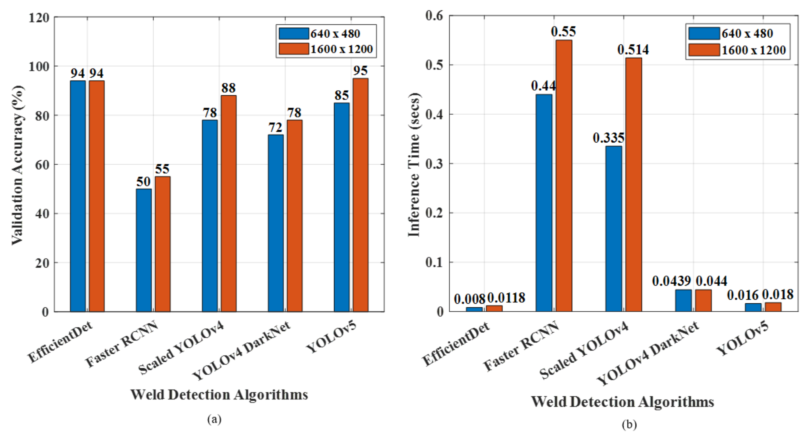
To further validate the generalisation ability, deep learning models were tested with datasets captured from a live camera which were not the part of test and validation datasets. The detection results are shown in Figure 14a–e. From the figure, it can be inferred that a live image of size 640 × 480 was used for testing and the weld shapes were classified into eight shapes with an accuracy of 90% using YOLOv5. Furthermore, the performance of the YOLO algorithms was compared with Faster RCNN and EfficientDet. It was seen that accuracy for all the shapes was 72%, which was comparatively lower than other models. Additionally, it took 1.5 h to train the network, but EfficientDet performed better with an accuracy of 95%. Additionally, the model performances of YOLO, EfficientDet and Faster RCNN were tested for different image sizes, namely, 640 × 480 and 1600 × 1200. These images were obtained from the GAN module and the 2D camera, so these sizes were taken for testing. The processing speed and validation accuracy were noted for each case, as shown in Figure 15a,b.
From the histogram, it can be seen that validation accuracy was high for the resolution of 1600 × 1200 using YOLOv5. Though the model was trained on 416 × 416, weld shapes were detected for both the image sizes. It was further noted that the higher the resolution, the better the classification was. Additionally, for higher pixels, the inference time for a single image was more than the image size of 640 × 480. However, detection was poor for Faster RCNN, as some shapes were misclassified and the bounding boxes did not exactly identify the weld shapes. Finally, an ablation study for the modules used in this work was conducted to demonstrate the needs of each module used. An ablation study at an architectural level will be considered in the future. For the analysis, nonhomogeneous weld fume images were taken to analyse the performance of detection with and without the denoising module. The performance was evaluated in terms of total time taken for the whole process and validation accuracy, which are listed in Table 8.
The total time was calculated based on pre-processing, GAN dehazing, the testing phase with 212 images of deep learning models, and contour detection for weld seam extraction. The training time was already listed in Table 7, so it was not considered. The validation accuracy was tested for nonhomogeneous weld fume images and dehazed images. It was found that accuracy was improved after dehazing the images. Additionally, PSNR was high for dehazed images with the value of 12.23, whereas it was low for fume images with the value of 11.44. This shows that the GAN module played a major role in accurate weld shape detection. It can be inferred that the total processing time taken for YOLOv5 with denoising and contour detection was 6.426 s, and for EfficientDet the total time was 7.185 s. The overall performance of weld detection was accurate for YOLOv5 and EfficientDet. The Faster RCNN processing time was high with the value of 44.626.

4.5. Coordinate Transformation Using the Artificial Neural Network

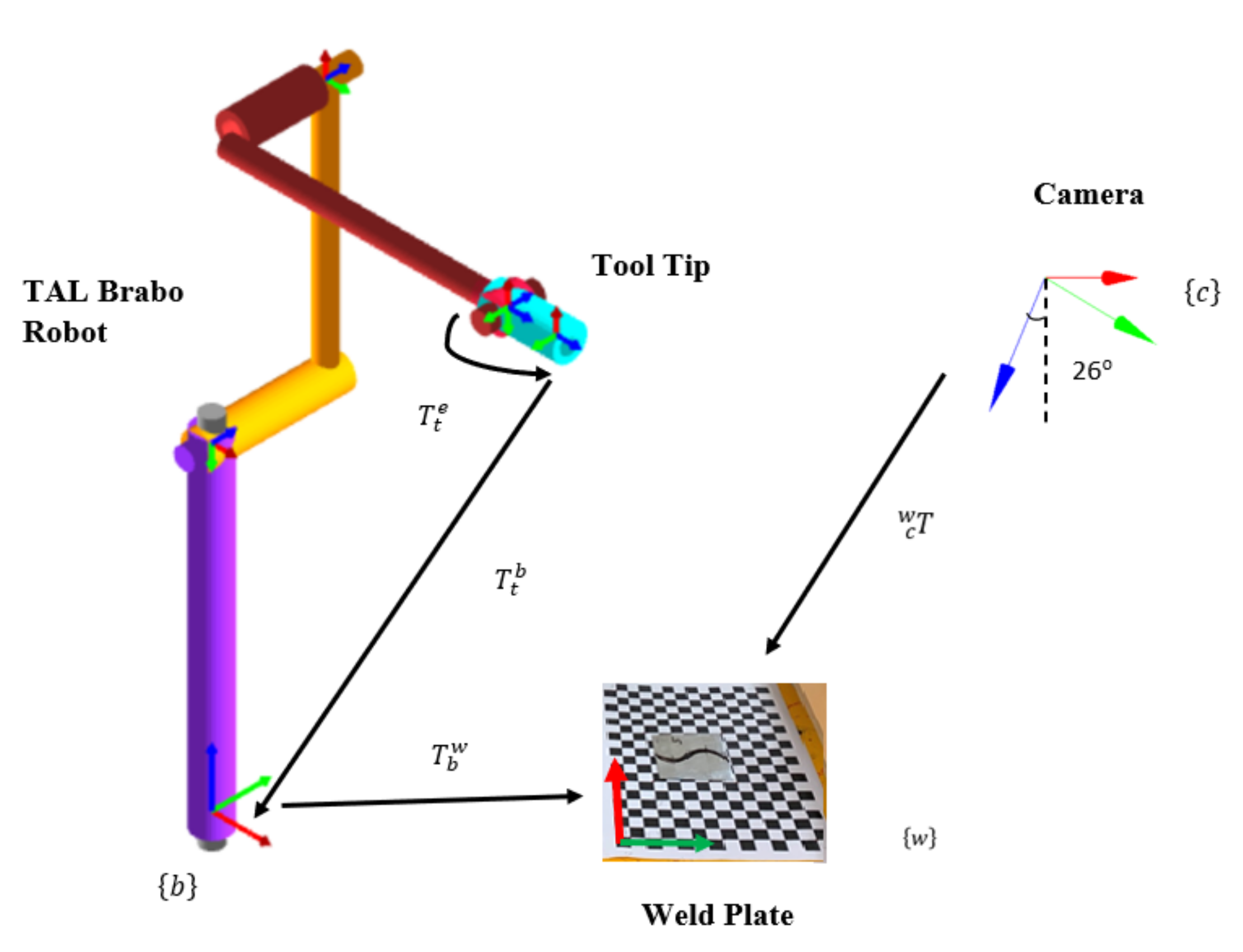
In every machine vision application, camera calibration is necessary to establish the relationship between three-dimensional world coordinates X ,   Y ,   Z and two-dimensional camera coordinates u , v , as well as determine the internal and external parameters of the camera [46]. In real-world scenarios, many factors can affect the process of robot vision caused by radial and tangential distortion, the position of the camera, the robot environment, and other dynamic objects, which in turn affects the experimental procedure. In general, camera calibration involves mathematical model formulation between the camera and the world, from which camera to base transformations or camera to robot end effector transformations are found out [47]. This involves the need to know the kinematics of the robot, which becomes tedious when the number of DOF increases, thereby increasing the complexity of the camera calibration. Additionally, when the camera setup is disturbed, the overall process has to be repeated, which becomes cumbersome. To eliminate such difficulties, the pixel coordinates of the calibration sheet T c w are mapped directly to robot coordinates T b w using neural networks; this does not need camera geometry information or complex mathematical equations, as shown in Figure 16. Using this approach, the coordinates of any object placed in robot workspace can be determined easily and efficiently.
In this work, the artificial neural network (ANN) model was developed to find the transformation between the camera and the world. The pixel coordinates ( x p ,   y p ) were taken as input and robot coordinates ( x i   ,   y i ) as output, with one hidden layer having 100 neurons. Initially, pixel input to the neural network model is given by
X i t = x p i ,   y p i   where = 1 , 2 , . , N s i z e   o f   i n p u t
The output of each neuron is given by
Y i t = f ( W i   t X i t + b )
where
W i   t = j = 1 N W i j t
Here, activation function is chosen as purelin, and it is given by f x = x .
Based on the initial weights, pixel inputs are updated at every time instant t .
X p i t + 1 = X p i t + j = 1 N W i j t
Once the inputs are updated, the weights are updated in next stage, which is given by
  W i   t + 1 =   W i   t + Δ W
Finally, the robot coordinates for the corresponding predicted robot coordinates are obtained, which is given by
Y r t = x r , y r
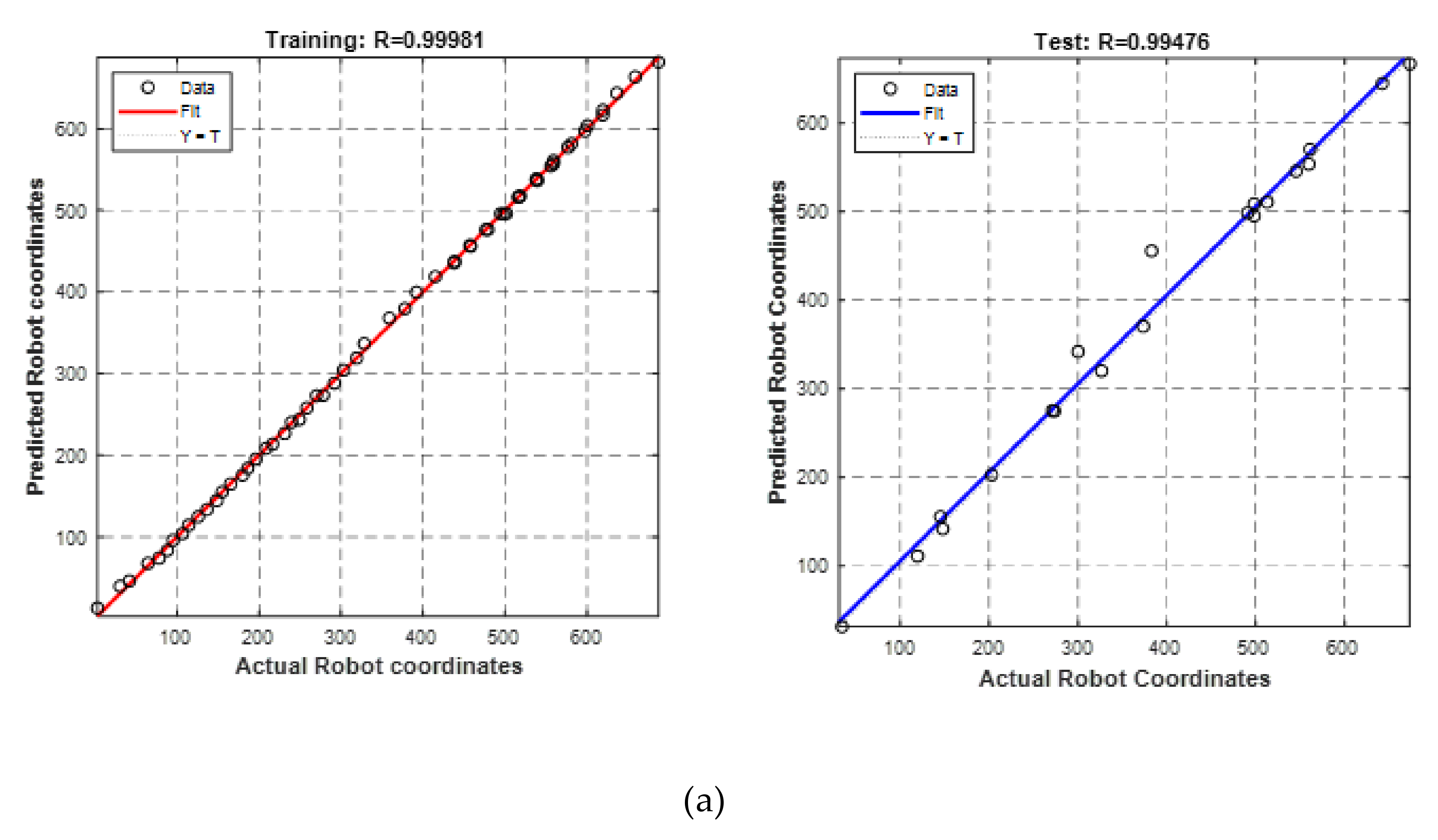
The size of the input (contour pixel coordinates) is 41 × 2 and the output size (robot coordinates) is 2 × 1. The Z value of the robot was fixed at the height of 230 mm for the safe operation of the robot and testing was performed in a planar environment. To find the effective training parameters for the neural network, the dataset was analysed with different combinations of training–testing–validation ratios, namely, 70-20-10, 80-10-10 and 50-25-25 and training functions trainscg, trainlm, trainrp and traingdx. The learning rate for the neural network was 0.001 with purelin as the activation function. The model was trained for 1000 epochs with a momentum coefficient of 0.9. The number of hidden layers for this analysis was chosen as 1, with 100 of hidden neurons to reduce the computation time and processing power. The corresponding Mean Square Error (MSE), Correlation Coefficient (R) value and Root Mean Square Error (RMSE) values are noted and are plotted for various combinations, as shown in Figure 17a,b. From the graph, the learning loss was comparatively less with the trainscg function and with the 50-25-25 ratio.
From the regression plot, it can be inferred that the R = 0.99981 value was higher for the 50-25-25 training–validation–testing ratio compared to other combinations, and also it had lower MSE and RMSE values of 230.6 and 15.18, respectively. Among the training functions, trainscg performed better and training was faster than the other functions. Additionally, trainlm, trainrp did not converge and training was stopped within 120 iterations out of 1000, leading to underfitting. traingdx was able to converge at 1000 epochs, but the RMSE and MSE values were huge, so it was not selected for training. The regression plot for training and testing for different combinations is illustrated in Figure 18. Finally, the contour pixels obtained from the contour detection algorithm were further converted to robot coordinates using the NN model, which was then sent to the robot via MATLAB for tracing the particular weld shape.
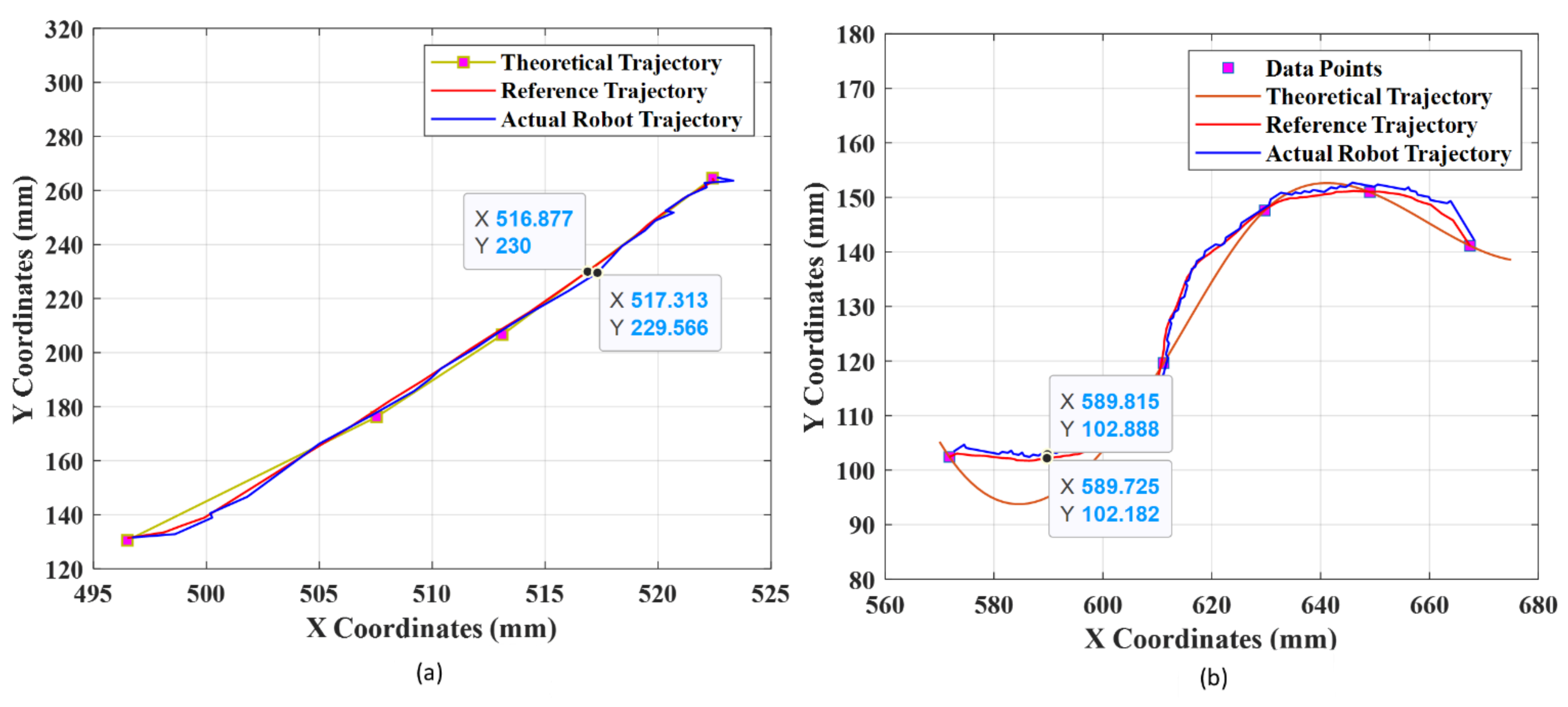
From the above ANN model hyperparameter analysis, it can be concluded that trainscg with the 50-25-25 data split performed best for the weld seam coordinates. Furthermore, in this work, to validate the real-time testing, the robot coordinates for shape 2 and shape 5 were obtained after transformation from the ANN model, and these coordinates were sent to the robot for tracing. The robot tracing path for the abovementioned shapes is shown in Figure 19. These trajectory points were recorded while the robot was tracing, and they were compared with the theoretical and actual trajectory points.
The theoretical trajectory for shape 2 (red line) was obtained using linear interpolation, whereas the reference trajectory (pink line) was obtained from the contour points. The robot-traced path is given by a blue line, and it can be inferred that for shape 2 the average tracking error between the reference and the actual path traced by the robot was 0.225 mm for X and 0.263 mm for the Y robot coordinates. The theoretical trajectory for shape 2 is as follows:
Y = 5.439 X + 2580.9
Similarly, the theoretical trajectory (red dotted line) for shape 5 was obtained by using the spline function to fit all the points, and it can be seen that the variation between the reference (pink line) and the actual trajectory traced by the robot (blue line) was about 0.299 mm for X and 0.114 mm for the Y robot coordinates. Therefore, the robot was able to trace the weld seam path obtained from the contour extraction with minimum error.

4.6. Comparison of Proposed Methodology with Previous Works

This section compares the present paperwork with other recent methods implemented in robotic welding using deep learning algorithms. An elaborate literature survey was carried out in the field of welding, dehazing methods, and deep learning architectures. Several works have been highlighted in Table 9.

5. Conclusions

To perform real-time intelligent robotic welding, weld seam detection using different algorithms such as Scaled YOLOv4, YOLOv5 and YOLOv4 DarkNet was proposed in this study. The problem of weld fumes was addressed in this work by performing image-to-image translation using DW-GAN. To extract the weld seam shape, binary thresholding-based contour detection was implemented; finally, to remove the difficulties of camera calibration and complex mathematical transformation, a neural network model was created to map the contour pixels into the robot coordinates and the robot was able to trace the weld seam accurately and precisely with less than a 1 mm tracking error. The main conclusions drawn from this experimental study are as follows:
  • Real-time weld datasets were collected, and were made of actual weld plates of mild steel. The total dataset for training the model comprised 2286 images with an image size of 416 × 416;
  • The weld fumes generally affected the detection performance; hence, DW-GAN was implemented to remove the weld fumes. The performance was compared with the conventional DCP method, and it was found that DW-GAN performed better for removing the fumes with PSNR 15.95 dB and SSIM 0.407. The inference time of DW-GAN was faster by 9.6 ms compared to DCP;
  • With the help of the YOLOv5 algorithm, the accurate and fast detection of weld seam shapes was realized with an overall inference speed of 0.0096 s, which was faster than Scaled YOLOv4 and YOLOv4 DarkNet. Additionally, the detection accuracy of YOLOv5 was 95%, with 96.7% precision, 96% recall, and 98.7% F1 score. The total loss of YOLOv5 was 0.043, whereas this was high for YOLOv4 DarkNet with the value of 0.959;
  • The YOLO algorithms were compared with Faster RCNN and EfficientDet and it was inferred that EfficientDet’s performance was similar to YOLOv5, and they outperformed other deep learning algorithms. The performance of the deep learning models was tested with different image sizes to validate the generalization ability, and weld plate detection was experimentally verified using live 2D camera images. The total processing time taken for YOLOv5 was just 6.426 s, which was less than that of the other deep learning methods;
  • An ablation study was performed to show the contribution of modules used in this work. The performance was analyzed in terms of validation accuracy and total time for the entire process. It was found that GAN played a major contribution in weld fume removal because accuracy was improved after dehazing;
  • The optimal combination of training parameters for NN was analyzed in terms of MSE, regression value, and RMSE, and it was found that the 50-25-25 training–validation–testing ratio with trainsscg was optimal for the efficient mapping of pixels into robot coordinates. The NN model made the coordinate transformation between the camera and the robot simpler, and this technique could be used in any machine vision application effectively and efficiently;
  • The contours present in the weld images were detected successfully and were sent to the robot using the trained NN model for simulated robotic welding via MATLAB. It was inferred that the accurate robot coordinates were obtained from the NN, which was helpful for accurate real-time weld shape tracing. The average tracking error was found to be less than 0.3 mm for all of the shapes.
Potential future works include the detection of weld seams with different brightness conditions, e.g., addressing arc lights and flash conditions. Additionally, segmentation-based detection could be implemented. Deep learning models could be further modified with different convolution layers, and their performance with weld datasets should be analyzed.

Author Contributions

Writing—original draft, A.S.; data curation, A.S. and A.D.; conceptualization, R.K.; formal analysis, V.K. and R.K.; methodology, A.S. and V.K.; software, A.S. and A.D.; supervision, V.K. and R.K.; validation, A.S. and A.D.; visualization, R.K.; writing—review and editing, V.K.; project Administration, V.K. All authors have read and agreed to the published version of the manuscript.

Funding

This research received no external funding.

Institutional Review Board Statement

Not Applicable.

Informed Consent Statement

Not Applicable.

Data Availability Statement

The datasets are available upon request.

Acknowledgments

The authors immensely grateful to the authorities of Birla Institute of Science and Technology Pilani, Dubai campus for their support throughout this research work.

Conflicts of Interest

The authors declare no conflict of interest.

Nomenclature

SymbolDescription
x L L , x L H , x H L , , and x H H Low pass and high pass filters
L t o t a l Total loss of DW-GAN
L s m o o t h Smooth loss
L M S S S I M Multi-scale structural similarity index loss
L p e r p e c t u a l Perceptual loss
L a d v Adversarial loss
α , β , γ Weighting factors
I Hazy image
K Haze free image
[ m   n ] Image size
l x , y Luminance function
c x , y Contrast function
s x , y Structure function
μ x , μ y Mean of x and y windows
σ x , σ y Covariance of x and y windows
σ x 2 ,   σ y 2 Variance of x and y windows
LDynamic pixel range
σ t x and σ t y Predictions of center with respect to anchor boxes
T c w Camera to world transformation
T b w Robot base to world transformation
X i t Pixel coordinates of Neural network
Y i t Output of each neurons
Y r t Final robot coordinates of neural network
W i t Layer weights
b bias
f Activation function
X i j Pixel inputs
C Number of Classes
c Confidence Score

References

  1. Sun, H.; Ma, T.; Zheng, Z.; Wu, M. Robot welding seam tracking system research basing on image identify. In Sensors and Smart Structures Technologies for Civil, Mechanical, and Aerospace Systems 2019; Lynch, J.P., Huang, H., Sohn, H., Wang, K.-W., Eds.; SPIE: Bellingham, WA, USA, 2019; pp. 864–870. [Google Scholar] [CrossRef]
  2. Ma, X.; Pan, S.; Li, Y.; Feng, C.; Wang, A. Intelligent welding robot system based on deep learning. In Proceedings of the 2019 Chinese Automation Congress (CAC), Hangzhou, China, 22–24 November 2019; pp. 2944–2949. [Google Scholar]
  3. Wang, X.; Zhou, X.; Xia, Z.; Gu, X. A survey of welding robot intelligent path optimization. J. Manuf. Process. 2021, 63, 14–23. [Google Scholar] [CrossRef]
  4. Zhang, H.; Song, W.; Chen, Z.; Zhu, S.; Li, C.; Hao, H.; Gu, J. Weld Seam Detection Method with Rotational Region Proposal Network. In Proceedings of the 2019 IEEE International Conference on Robotics and Biomimetics (ROBIO), Dali, China, 6–8 December 2019; pp. 2152–2156. [Google Scholar]
  5. Mohd Shah, H.N.; Sulaiman, M.; Shukor, A.Z. Autonomous detection and identification of weld seam path shape position. Int. J. Adv. Manuf. Technol. 2017, 92, 3739–3747. [Google Scholar] [CrossRef]
  6. Li, W.; Cao, G.; Sun, J.; Liang, Y.; Huang, S. A calibration algorithm of the structured light vision for the arc welding robot. In Proceedings of the 2017 14th International Conference on Ubiquitous Robots and Ambient Intelligence (URAI), Jeju, Korea, 28 June–1 July 2017; pp. 481–483. [Google Scholar]
  7. Shao, W.; Liu, X.; Wu, Z. A robust weld seam detection method based on particle filter for laser welding by using a passive vision sensor. Int. J. Adv. Manuf. Technol. 2019, 104, 2971–2980. [Google Scholar] [CrossRef]
  8. Lei, T.; Huang, Y.; Wang, H.; Rong, Y. Automatic weld seam tracking of tube-to-tubesheet TIG welding robot with multiple sensors. J. Manuf. Process. 2021, 63, 60–69. Available online: https://www.sciencedirect.com/science/article/pii/S1526612520301870 (accessed on 14 April 2022). [CrossRef]
  9. Yin, Z.; Ma, X.; Zhen, X.; Li, W.; Cheng, W. Welding Seam Detection and Tracking Based on Laser Vision for Robotic Arc Welding. J. Phys. Conf. Ser. IOP Publ. 2020, 1650, 022030. [Google Scholar] [CrossRef]
  10. Zou, Y.; Zhou, W. Automatic seam detection and tracking system for robots based on laser vision. Mechatronics 2019, 63, 102261. Available online: https://www.sciencedirect.com/science/article/pii/S0957415819300947 (accessed on 2 May 2022). [CrossRef]
  11. Zhang, X.; Xu, Z.; Xu, R.; Liu, J.; Cui, P.; Wan, W.; Sun, C.; Li, C. Towards Domain Generalization in Object Detection. arXiv 2022, arXiv:2203.14387. [Google Scholar]
  12. Zou, Y.; Lan, R.; Wei, X.; Chen, J. Robust seam tracking via a deep learning framework combining tracking and detection. Appl. Opt. 2020, 59, 4321–4331. Available online: http://ao.osa.org/abstract.cfm?URI=ao-59-14-4321 (accessed on 12 May 2022). [CrossRef]
  13. Xu, Y.; Wang, Z. Visual sensing technologies in robotic welding: Recent research developments and future interests. Sens. Actuators A Phys. 2021, 320, 112551. [Google Scholar] [CrossRef]
  14. Nowroth, C.; Gu, T.; Grajczak, J.; Nothdurft, S.; Twiefel, J.; Hermsdorf, J.; Hermsdorf, J.; Kaierle, S.; Wallaschek, J. Deep Learning-Based Weld Contour and Defect Detection from Micrographs of Laser Beam Welded Semi-Finished Products. Appl. Sci. 2022, 12, 4645. [Google Scholar] [CrossRef]
  15. Lei, T.; Rong, Y.; Wang, H.; Huang, Y.; Li, M. A review of vision-aided robotic welding. Comput. Ind. 2020, 123, 1–30. [Google Scholar] [CrossRef]
  16. Singh, D.; Kumar, V. A comprehensive review of computational dehazing techniques. Arch. Comput. Methods Eng. 2019, 26, 1395–1413. [Google Scholar] [CrossRef]
  17. Long, J.; Shi, Z.; Tang, W.; Zhang, C. Single remote sensing image dehazing. IEEE Geosci. Remote Sens. Lett. 2013, 11, 59–63. [Google Scholar] [CrossRef]
  18. Sindagi, V.A.; Oza, P.; Yasarla, R.; Patel, V.M. Prior based domain adaptive object detection for hazy and rainy conditions. In Proceedings of the European Conference on Computer Vision, Glasgow, UK, 23–28 August 2020; pp. 763–780. [Google Scholar]
  19. Katyal, S.; Kumar, S.; Sakhuja, R.; Gupta, S. Object detection in foggy conditions by fusion of saliency map and yolo. In Proceedings of the 2018 12th International Conference on Sensing Technology (ICST), Limerick, Ireland, 3–6 December 2018; pp. 154–159. [Google Scholar]
  20. Fu, M.; Liu, H.; Yu, Y.; Chen, J.; Wang, K. DW-GAN: A Discrete Wavelet Transform GAN for NonHomogeneous Dehazing. In Proceedings of the IEEE/CVF Conference on Computer Vision and Pattern Recognition, Nashville, TN, USA, 20–25 June 2021; pp. 203–212. [Google Scholar]
  21. Ghate, S.N.; Nikose, M.D. New Approach to Underwater Image Dehazing using Dark Channel Prior. J. Phys. Conf. Ser. 2021, 1937, 012045. [Google Scholar] [CrossRef]
  22. Creswell, A.; White, T.; Dumoulin, V.; Arulkumaran, K.; Sengupta, B.; Bharath, A.A. Generative adversarial networks: An overview. IEEE Signal Process. Mag. 2018, 35, 53–65. [Google Scholar] [CrossRef] [Green Version]
  23. Isola, P.; Zhu, J.Y.; Zhou, T.; Efros, A.A. Image-to-image translation with conditional adversarial networks. In Proceedings of the IEEE Conference on Computer Vision and Pattern Recognition, Honolulu, HI, USA, 21–26 July 2017; pp. 1125–1134. [Google Scholar]
  24. Liu, M.-Y.; Tuzel, O. Coupled generative adversarial networks. arXiv 2016, arXiv:1606.07536. [Google Scholar]
  25. Ledig, L.C.; Theis, F.; Huszar, J.; Caballero, A.; Cunningham, A.; Acosta, A.; Aitken, A.; Tejani, J.; Totz, Z.; Wang, S.; et al. Photo-realistic single image super-resolution using a generative adversarial network. In Proceedings of the IEEE Conference on Computer Vision and Pattern Recognition, Honolulu, HI, USA, 21–26 July 2017; pp. 4681–4690. [Google Scholar]
  26. Deng, Q.; Huang, Z.; Tsai, C.-C.; Lin, C.-W.; Hardgan, A. Haze-aware representation distillation gan for single image dehazing. In Proceedings of the European Conference on Computer Vision, Glasgow, UK, 23–28 August 2020; pp. 722–738. [Google Scholar]
  27. Zhang, H.; Sindagi, V.; Patel, V.M. Image de-raining using a conditional generative adversarial network. IEEE Trans. Circuits Syst. Video Technol. 2019, 30, 3943–3956. [Google Scholar] [CrossRef] [Green Version]
  28. Pintor, M.; Angioni, D.; Sotgiu, A.; Demetrio, L.; Demontis, A.; Biggio, B.; Roli, F. ImageNet-Patch: A Dataset for Benchmarking Machine Learning Robustness against Adversarial Patches. arXiv 2022, arXiv:2203.04412. [Google Scholar]
  29. Das, A.; Chandran, S. Transfer learning with res2net for remote sensing scene classification. In Proceedings of the 2021 11th International Conference on Cloud Computing, Data Science & Engineering (Confluence), Noida, India, 28–29 January 2021; pp. 796–801. [Google Scholar]
  30. Kan, S.; Zhang, Y.; Zhang, F.; Cen, Y.A. GAN-based input-size flexibility model for single image dehazing. Signal Process. Image Commun. 2022, 102, 116599. [Google Scholar] [CrossRef]
  31. Chaitanya, B.S.N.V.; Mukherjee, S. Single image dehazing using improved cycleGAN. J. Vis. Commun. Image Represent. 2021, 74, 103014. [Google Scholar] [CrossRef]
  32. Srivastava, S.; Divekar, A.V.; Anilkumar, C.; Naik, I.; Kulkarni, V.; Pattabiraman, V. Comparative analysis of deep learning image detection algorithms. J. Big Data 2021, 8, 1–27. [Google Scholar] [CrossRef]
  33. Zuo, Y.; Wang, J.; Song, J. Application of YOLO Object Detection Network In Weld Surface Defect Detection. In Proceedings of the 2021 IEEE 11th Annual International Conference on CYBER Technology in Automation, Control and Intelligent Systems (CYBER), Jiaxing, China, 27–31 July 2021; pp. 704–710. [Google Scholar]
  34. Wu, D.; Lv, S.; Jiang, M.; Song, H. Using channel pruning-based YOLO v4 deep learning algorithm for the real-time and accurate detection of apple flowers in natural environments. Comput. Electron. Agric. 2020, 178, 105742). Available online: https://www.sciencedirect.com/science/article/pii/S0168169920318986 (accessed on 15 April 2022). [CrossRef]
  35. Jiang, Z.; Zhao, L.; Li, S.; Jia, Y. Real-time object detection method based on improved YOLOv4-tiny. arXiv 2020, arXiv:2011.04244. [Google Scholar]
  36. Liang, T.J.; Pan, W.G.; Bao, H.; Pan, F. Vehicle wheel weld detection based on improved YO-LO v4 algorithm. Comp. Opt. 2022, 46, 271–279. [Google Scholar] [CrossRef]
  37. Jiang, P.; Ergu, D.; Liu, F.; Cai, Y.; Ma, B.A. Review of Yolo Algorithm Developments. Proc. Comp. Sci. 2022, 199, 1066–1073. [Google Scholar] [CrossRef]
  38. Gong, X.-Y.; Su, H.; Xu, D.; Zhang, Z.-T.; Shen, F.; Yang, H.-B. An Overview of Contour Detection Approaches. Int. J. Autom. Comput. 2018, 15, 656–672. [Google Scholar] [CrossRef]
  39. Ghiasi, G.; Lin, T.Y.; Le, Q.V. Dropblock: A regularization method for convolutional networks. Adv. Neural. Inf. Process. Syst. 2018, 31, 12890. [Google Scholar] [CrossRef]
  40. Zheng, Q.; Yang, M.; Tian, X.; Jiang, N.; Wang, D. A full stage data augmentation method in deep convolutional neural network for natural image classification. Discret. Dyn. Nat. Soc. 2020, 2020, 4706576. [Google Scholar] [CrossRef]
  41. Bian, Y.C.; Fu, G.H.; Hou, Q.S.; Sun, B.; Liao, G.L.; Han, H.D. Using Improved YOLOv5s for Defect Detection of Thermistor Wire Solder Joints Based on Infrared Thermography. In Proceedings of the 2021 5th International Conference on Automation, Control and Robots (ICACR), Nanning, China, 25–27 September 2021; pp. 29–32. [Google Scholar]
  42. Song, Q.; Li, S.; Bai, Q.; Yang, J.; Zhang, X.; Li, Z.; Duan, Z. Object Detection Method for Grasping Robot Based on Improved YOLOv5. Micromachines 2021, 12, 1273. [Google Scholar] [CrossRef]
  43. Zhu, C.; Yuan, H.; Ma, G. An active visual monitoring method for GMAW weld surface defects based on random forest model. Mat. Res. Exp. 2022, 9, 036503. [Google Scholar] [CrossRef]
  44. Yu, J.; Zhang, W. Face mask wearing detection algorithm based on improved YOLO-v4. Sensors 2021, 21, 3263. [Google Scholar] [CrossRef] [PubMed]
  45. Chuang, J.H.; Ho, C.H.; Umam, A.; Chen, H.Y.; Hwang, J.N.; Chen, T.A. Geometry-based camera calibration using closed-form solution of principal line. IEEE Trans. Image Process. 2021, 30, 2599–2610. [Google Scholar] [CrossRef] [PubMed]
  46. Vo, M.; Wang, Z.; Luu, L.; Ma, J. Advanced geometric camera calibration for machine vision. Opt. Eng. 2011, 50, 11503. [Google Scholar] [CrossRef] [Green Version]
  47. Segota, S.B.; Anđelic, N.; Mrzljak, V.; Lorencin, I.; Kuric, I.; Car, Z. Utilization of multilayer perceptron for determining the inverse kinematics of an industrial robotic manipulator. Int. J. Adv. Robot. Syst. 2021, 18, 1729881420925283. [Google Scholar] [CrossRef]
  48. Liu, C.; Chen, S.; Huang, J. Machine Vision-Based Object Detection Strategy for Weld Area. Sci. Program. 2022, 2022, 1188974. [Google Scholar] [CrossRef]
  49. Ma, G.; Yu, L.; Yuan, H.; Xiao, W.; He, Y. A vision-based method for lap weld defects monitoring of galvanized steel sheets using convolutional neural network. J. Manuf. Proc. 2021, 64, 130–139 . [Google Scholar] [CrossRef]
  50. Yun, G.H.; Oh, S.J.; Shin, S.C. Image Preprocessing Method in Radiographic Inspection for Automatic Detection of Ship Welding Defects. Appl. Sci. 2021, 12, 123. [Google Scholar] [CrossRef]
  51. Li, R.; Gao, H. Denoising and feature extraction of weld seam profiles by stacked denoising autoencoder. Weld World 2021, 65, 1725–1733. [Google Scholar] [CrossRef]
  52. Shao, W.; Rong, Y.; Huang, Y. Image contrast enhancement and denoising in micro-gap weld seam detection by periodic wide-field illumination. J. Manuf. Processes 2022, 75, 792–801. [Google Scholar] [CrossRef]
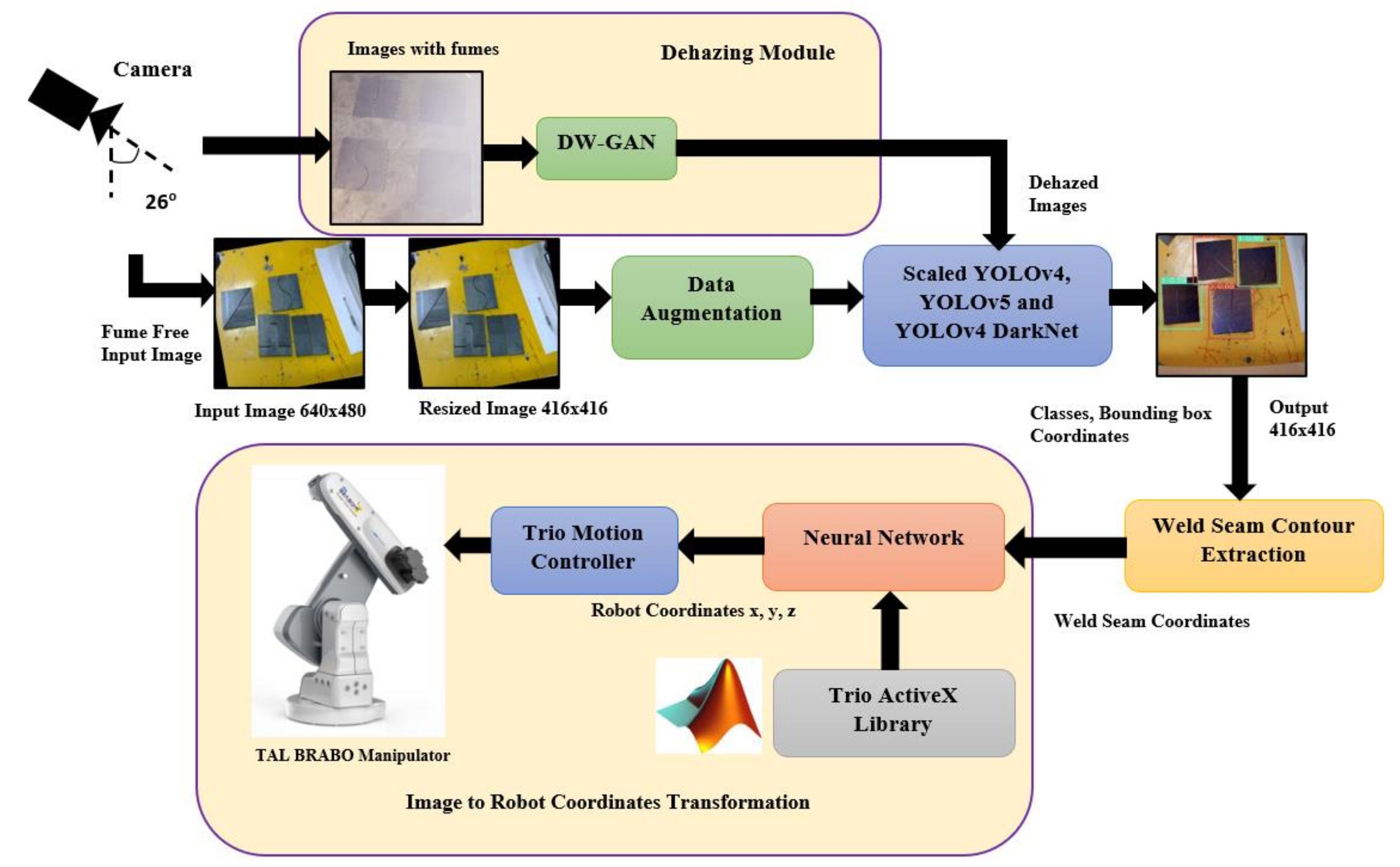
Figure 1. Process flow diagram of weld seam detection and tracing using TAL BRABO robotic manipulator.
Applsci 12 06860 g001
Figure 2. Actual weld seam datasets with weld fumes, flip, and rotate conditions for training YOLO Algorithms.
Applsci 12 06860 g002
Figure 3. DW-GAN architecture for weld fume removal.
Applsci 12 06860 g003
Figure 4. Res2Net architecture used in knowledge adaption branch [28].
Applsci 12 06860 g004
Figure 5. YOLOv4 architecture for weld seam detection and tracing.
Applsci 12 06860 g005
Figure 6. YOLOv5 architecture for weld seam detection and tracing.
Applsci 12 06860 g006
Figure 7. Process flow diagram of Scaled Yolov4-based weld seam detection and tracing.
Applsci 12 06860 g007
Figure 8. Real-time hardware setup of TAL BRABO manipulator for weld seam detection and tracing.
Applsci 12 06860 g008
Figure 9. Comparison of weld fume removal using (af) Ground Truth Image (gl) DW-GAN and (mr) DCP methods.
Applsci 12 06860 g009
Figure 10. Image histogram to show the comparison between (a) ground truth (b) DCP (c) DW-GAN.
Applsci 12 06860 g010
Figure 11. Performance evaluation of weld fumes removal (a) PSNR (b) SSIM (c) MSE and (d) NIQE.
Applsci 12 06860 g011
Figure 12. Mild steel plates with different shape numbers used for YOLO training and real-time experimental validation.
Applsci 12 06860 g012
Figure 13. Real-time weld seam detection: (ae) YOLOv5; (dh) Scaled YOLOv4; (im) YOLOv4 DarkNet.
Applsci 12 06860 g013
Figure 14. Generalization test of deep learning models: (a) YOLOv5; (b) Scaled YOLOv4; (c) YOLOv4 DarkNet; (d) Faster RCNN (e) EfficientDet.
Applsci 12 06860 g014
Figure 15. Deep learning model performance for different image sizes: (a) validation accuracy; (b) inference time.
Applsci 12 06860 g015
Figure 16. Coordinate transformation between camera and weld plate with respect to robot base.
Applsci 12 06860 g016
Figure 17. (a) Graph of training functions vs. MSE and RMSE; (b) graph of different training–validation–testing ratios vs. MSE and RMSE.
Applsci 12 06860 g017
Figure 18. (a) Regression plot for 50-25-25; (b) regression plot for 70-10-20; (c) regression plot for 80-10-10.
Applsci 12 06860 g018aApplsci 12 06860 g018b
Figure 19. (a) Real-time path traced by the robot for shape 4; (b) real-time path traced by the robot for shape 5.
Applsci 12 06860 g019
Table 1. Weld plate and data augmentation specifications for data acquisition.
ParameterValues
Width (mm)100
Height (mm)100
Weld gap (mm)2
FlipHorizontal, Vertical
Rotate   90 ° Clockwise
Rotation 15 ° to   + 15 °
Grayscale11%
Saturation−30% to +30%
Table 2. U-Net architecture using the DWT branch.
Contracting PathExpansive Path
LayerDetailsOutput SizeLayerDetailsOutput Size
InputWeld Images572 × 572 × 3DWT UpSampling_12 × 2 × 1024 up sample of Conv5_2;
Concat with Conv4_2
56 × 56
Conv1_13 × 3 × 64; Linear ReLU570 × 570Conv6_13 × 3 × 512; Linear ReLU54 × 54
Conv1_23 × 3 × 64; Linear ReLU570 × 570Conv6_23 × 3 × 512; Linear ReLU52 × 52
Pool 12 × 2 Max Pool
Stride 2
284 × 284DWT UpSampling_22 × 2 × 512 up sample of Conv6_2;
Concat with Conv3_2
104 × 104
Conv2_13 × 3 × 128; Linear ReLU284 × 284Conv7_13 × 3 × 256; Linear ReLU102 × 102
Conv2_23 × 3 × 128; Linear ReLU282 × 282Conv7_23 × 3 × 256; Linear ReLU100 × 100
Pool 22 × 2 Max Pool
Stride 2
140 × 140DWT UpSampling_32 × 2 × 256 up sample of Conv7_2;
Concat with Conv2_2
200 × 200
Conv3_13 × 3 × 256; Linear ReLU138 × 138Conv8_13 × 3 × 128; Linear ReLU198 × 198
Conv3_23 × 3 × 256; Linear ReLU136 × 136Conv8_23 × 3 × 128; Linear ReLU196 × 196
Pool 32 × 2 Max Pool
Stride 2
68 × 68DWT UpSampling_42 × 2 × 128 up sample of Conv1_2;
Concat with Conv2_2
392 × 392
Conv4_13 × 3 × 512; Linear ReLU66 × 66Conv9_13 × 3 × 64; Linear ReLU390 × 390
Conv4_23 × 3 × 512; Linear ReLU64 × 64Conv9_23 × 3 × 64; Linear ReLU388 × 388
Pool 42 × 2 Max Pool
Stride 2
32 × 32Conv101 × 1 × 2; Linear ReLU388 × 388
Conv5_13 × 3 × 1024; Linear ReLU30 × 30
Conv5_23 × 3 × 1024; Linear ReLU28 × 28
Table 3. Knowledge adaption architecture using Res2Net.
LayerDetailsOutput Size
InputWeld Images572 × 572 × 3
Res2Net_13 Conv Layers 3 × 3 × 64
3 × 3 × 128; 3 × 3 × 256
566 × 566
Res2Net_23 Conv Layers 3 × 3 × 64
3 × 3 × 128; 3 × 3 × 256
281 × 281
Res2Net_33 Conv Layers 3 × 3 × 64
3 × 3 × 128; 3 × 3 × 256
134 × 134
Attention Module_03 × 31024 × 1024
Pixel ShuffleUpscale factor = 2
Attention Module_13 × 3256 × 256
Upsampling_12 × 2; concat with Res2Net_2
Pixel ShuffleUpscale factor = 2
Attention Module_23 × 3192 × 192
Upsampling_22 × 2; concat with Res2Net_1
Pixel ShuffleUpscale factor = 2
Attention Module_33 × 3112 × 112
Upsampling_32 × 2; concat with Input layer
Pixel ShuffleUpscale factor = 2
Attention Module_43 × 344 × 44
Conv_13 × 3 × 4444 × 44
Conv_23 × 3 × 4428 × 28
Table 4. Layers of discriminator architecture.
LayerDetailsOutput Size
Conv_13 × 3 × 3; padding = 1
Leaky ReLU
64 × 64
Conv_23 × 3 × 64; padding = 1
Leaky ReLU; stride = 2
64 × 64
Conv_33 × 3 × 64; padding = 1
Leaky ReLU
128 × 128
Conv_43 × 3 × 64; padding = 1
Leaky ReLU; stride = 2
128 × 128
Conv_53 × 3 × 128; padding = 1
Leaky ReLU
256 × 256
Conv_63 × 3 × 256; padding = 1
Leaky ReLU; stride = 2
256 × 256
Conv_73 × 3 × 256; padding = 1
Leaky ReLU
512 × 512
Conv_83 × 3 × 512; padding = 1
Leaky ReLU; stride = 2
512 × 512
Conv_91 × 1 × 512
Leaky ReLU
1024 × 1024
Conv_101x 1 × 1024
Leaky ReLU
1 × 1
Table 5. Hardware configuration and deep learning environment.
S. NoEnvironmentValues/Version
1Operating SystemWindows 11
2CPUIntel(R) Core(TM) i7-9750H CPU @ 2.60 GHz 2.59 GHz
3GPUTesla P100-PCIE-16 GB
4RAM/ROM2666 MHz DDR4 16 GB
5CUDA11.2
6cuDNN 7.6.5
7IDEColab Pro Plus
8Frameworkpytorch
Table 6. Initial and final training parameters of different YOLO algorithms.
S. NoParameterInitial ValueOptimized Value (YOLOv4)Optimized Value (YOLOv5)
1Learning rate0.010.01210.0108
2Momentum constant0.930.9370.98
3Weight decay0.00050.000390.00035
4Class loss0.51.091.42
5IoU_target0.20.20.2
6Anchor_target44.63.88
7Epochs50200200
8Dataset Split ratio60-20-2060-20-2060-20-20
Table 7. Performance metrics of different YOLO algorithms during weld shape detection.
S. NoParameterScaled YOLOv4YOLOv5YOLOv4 DarkNetFaster RCNNEfficientDet
1Precision0.760.9670.470.50.788
2Recall0.9830.960.470.50.841
3mAP0.9730.9870.5340.540.92
4F1 score0.850.960.540.50.813
5GIoU loss0.0230.0170.3170.5410.00089
6Object loss0.0710.0220.3020.50840.133
7Class loss0.0150.00460.340.2120.169
8Training Time (h)0.9010.7100.5341.50.583
9GPU memory5.51 GB1.89 GB1.70 GB6.7 GB1.5 GB
10Total Loss0.1090.04360.9591.2610.303
Table 8. Ablation study of weld shape detection.
S. NoModulesTotal Time (s)Validation Accuracy (%)
1Pre-processing + Scaled YOLOv4 + Contour detection4.38781
2Pre-processing + Scaled YOLOv4 + GAN dehazing + Contour detection 10.71785
3Pre-processing + YOLOv5 + Contour detection0.096782
4Pre-processing + YOLOv5 + GAN dehazing + Contour detection6.42689
5Pre-processing + YOLOv4 DarkNet + Contour detection20.82870
6Pre-processing + YOLOv4 DarkNet + GAN dehazing + Contour detection27.15876
7Pre-processing + Faster RCNN + Contour detection38.29653
8Pre-processing + Faster RCNN + GAN dehazing + Contour detection44.62661
9Pre-processing + EfficientDet + Contour detection0.85589
10Pre-processing + EfficientDet + GAN dehazing + Contour detection7.18593
Table 9. Comparison of present work with previous methods.
S.NOAuthorMethodologyPerformance MetricsTracking Error
1Yanbiao Zou et al., 2019 [11]DCNN with VGGNet
Weld seam searching with arc and splash noise
Inf time (356 images): 15.06 secLess than 1 mm
2Chenhua Liu et al., 2022 [48]Faster RCNN with different RPN networksValidation accuracy: 86.45%
Inference time: 25.02 ms
-
3GuohongMa et al., 2021 [49]CNN with AlexNet and VGG16Accuracy: AlexNet: 95.83%, VGG16: 89.17%
Recall: 100%
-
4Gwang-ho Yun et al., 2022 [50]Contrast limited adaptive histogram equalization (CLAHE) and image denoising
YOLO
Loss: 0.03415
mAP: 51.2%
-
5Ran Li et al., 2021 [51]Stacked denoising autoencoder (SDAE) for GMAW weldingAverage error: 0.086-
6Shao W et al., 2022 [52]Periodic wide-field illuminationSNR: 35%-
7Present MethodDWT-GAN for dehazing
And YOLOv5
PSNR (GAN): 15.95
SSIM (GAN): 0.407
Validation Accuracy: 95%
Total loss: 0.043
Inf time (212 images): 9.6 ms
Less than 0.3 mm
Publisher’s Note: MDPI stays neutral with regard to jurisdictional claims in published maps and institutional affiliations.