Abstract
We present a fast 3D analytical affine transformation (F3DAAT) method to obtain polygon-based computer-generated holograms (CGHs). CGHs consisting of tens of thousands of triangles from 3D objects are obtained by this method. We have attempted a revised method based on previous 3D affine transformation methods. In order to improve computational efficiency, we have derived and analyzed our proposed affine transformation matrix. We show that we have further increased the computational efficiency compared with previous affine methods. We also have added flat shading to improve the reconstructed image quality. A 3D object from a 3D camera is reconstructed holographically by numerical and optical experiments.
1. Introduction
With the rapid development of display and computer technology, 3D display technology has made great progress [,]. The current 3D display technologies generally include binocular parallax display [], volume 3D display [], light field display [] and holographic 3D display. Holographic 3D display is a technology to reconstruct 3D wave-front by using light wave diffraction information based on the principle of wave optics. Because the wave-front information of the 3D scene is reconstructed, it can provide all the depth cues required by the human eye [,,]. The wave-front recording process of holography can be completed and simulated by a computer to generate the so-called computer-generated holograms (CGHs). The use of CGHs avoids the setup of complicated optical paths in optical holography [,], as long as the mathematical description of the 3D scene is obtained and transformed into the wave-front distribution in the hologram plane by algorithms. Therefore, the algorithm of calculating CGHs is key, because it directly determines the computational efficiency of the hologram and the quality of the reconstructed image [,].
Indeed, the mathematical description of a 3D scene can also be expressed in many forms. According to the geometric information of its surface, it can be discretely expressed as a collection of point sources, giving the so-called point-based method []. The wavefront information of the whole 3D object is obtained by calculating and then adding the light field distribution of the spherical wave emitted by each point light source in the hologram plane. However, the required number of point sources is usually as high as millions, leading to computational bottlenecks. By using a look-up tables (LUTs) [,,] and graphic processing units (GPUs) [,], we can accelerate the calculations greatly. Another popular CGH calculation method is the use of polygons (usually represented by triangle meshes) to approximate the surface of a 3D scene, giving to the polygon-based method [,,,,,,,,,,,,,]. Compared with the point-based method, the number of polygons can be greatly reduced, and the mature theory of computer graphics can be used to make the reconstructed scene more realistic. There are other methods to decompose 3D objects, such as the layer-based [,] or line-segment based method [].
In polygon-based methods, the propagation of light field can be calculated for each polygon by using the angular spectrum theory if the polygon is parallel to the hologram plane []. The essence of polygon-based methods is the diffraction calculation between non-parallel planes. Polygon-based methods can be divided into two categories; one is the traditional method based on sampling []. This method needs to sample each tilted polygon that is not parallel to the hologram in the spatial and frequency domains. Due to the polygon rotation, sampling in the spatial and frequency domains creates uneven sampling intervals between the two domains. Time-consuming interpolation is needed to alleviate sampling distortion. The other method is the analytical method []. Unlike the traditional method, sampling in the spatial domain to obtain the spectrum of a tilted polygon is not needed. Instead, the spectrum of a tilted polygon can be expressed in terms of the spectrum of a unit triangle (also called primitive triangle), which is known analytically, through the 2D affine transform []. Therefore, only sampling is needed in the frequency domain for each polygon, bypassing the need for interpolation in the traditional method. Compared with the traditional method, the analytical method effectively reduces the amount of calculations. However, shaping and texture mapping are not easily included in the analytical methods as compared with the traditional methods [].
Pan et al. [,] have developed an analytical method utilizing 3D affine transformation. They have defined a pseudo inverse matrix to map the spatial triangle with a three-dimensional right primitive triangle (which has an analytical spectrum expression). The major issue of the technique is the inaccuracy caused by the inversion of the pseudo matrix. Zhang et al. [,] have derived a correct analytical expression in the context of 2D affine transformation [] and proposed a method to achieve 3D transformation from an arbitrary triangle to a primitive triangle through a 3D rotation of the arbitrary triangle and the use of a 2D affine matrix []. Although this method avoids the time-consuming calculation of the pseudo inverse matrix, the process is rather complex. Zhang et al. [] also have proposed a method called the fast 3D affine transformation (F3DAT) method by translating the primitive triangle to avoid the use of the pseudo inverse matrix to improve the computational efficiency.
In the wave-optics based approach, it can provide accurate depth cues. However, view-dependent properties’ rendering requires additional calculations. Rendering technology of computer graphics makes the reconstructed 3D scene more realistic [,,]. Matsushima et al., have discussed the methods of shading and texturing [,,] and created a large-scale full-color CGH successfully []. Subsequently, many methods have been proposed to improve the quality of reconstructed images through texturing [,], shading [,], and resolution improvement []. Additionally, the use of the silhouette method for hidden surface removal has been described [].
In this study, based on the three-dimensional affine theory [,], we present a fast 3D analytical affine transformation (F3DAAT) method to obtain a full-analytical spectrum of a spatial triangle. We obtain the analytical expression of a 3D affine matrix algebraically, and the spectrum of tilted triangles can be obtained directly. Compared with previous methods, we show improved computational efficiency. In addition, in order to improve the image quality, we add flat shading to make the reconstructed image more realistic. We also demonstrate reconstructed 3D objects composed of tens of thousands of polygons numerically as well as the use of a spatial light modulator (SLM) for optical reconstruction.
In Section 2, we briefly introduce the basic principle of the polygon-based method. In Section 3, we present the theory of F3DAAT. In Section 4, we demonstrate the reconstruction of 3D objects numerically and optically. The computational efficiency is also compared with previous methods. The results of adding flat shading are also illustrated.
2. Conventional Polygon-Based Method
Figure 1 shows the basic principle of the polygon-based method. The surface of a 3D object is discretized into many polygons (usually triangles). The hologram is assumed to be on the plane . The total complex field distribution on the hologram plane can be expressed as the superposition of the polygon fields from each polygon, :
where is the number of polygons and is the complex field on the hologram plane from the polygon. Since the complex field distribution of each triangle on the hologram can be expressed by the inverse Fourier transform of its spectrum:
where represent the inverse Fourier transform and represents the spectrum of the polygon on the hologram. Therefore, the key to the polygon-based method is how to obtain the spectrum of each triangle on the hologram plane.
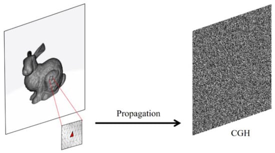
Figure 1.
Principle of the polygon-based method.
As shown in Figure 2, a polygon on the source coordinate system is not necessarily parallel to the hologram plane ; one needs to rotate the polygon to parallel local coordinate system to be parallel to the hologram plane in order to calculate the diffracted field toward the hologram through standard diffraction theory []. The spatial frequencies can be expressed as:
where are the elements of the rotation matrix. (corresponding to in Equation (10a,b) in Ref. []) are the spatial frequencies corresponding to source coordinates . (corresponding to in Equation (10a,b) in Ref. []) are spatial frequencies corresponding to parallel local coordinates . Upon a differential operation in Equation (3a), we have:
where with being the wavelength of the light source. Since the spatial frequencies are uniformly distributed, we have For simplicity, let us assume and Equation (4) then can be rewritten as follows:
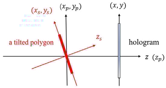
Figure 2.
Coordinate systems of the traditional polygon-based method: source coordinate system , parallel local coordinate system and hologram plane Adapted from Zhang et al. [].
Since (the derivative of ) is not constant, Equation (5) indicates that for an arbitrary set of spatial frequencies corresponding to the parallel local coordinates, spatial frequency after rotation has highly nonlinear properties. Because uniform sampling is necessary for the FFT to work correctly in the traditional method, interpolation process is required for spatial frequencies after rotation. This procedure would add substantially to the computational time []. Comparing with the traditional method, the analytical method avoids the use of the FFT in obtaining the spectrum of the polygon in the source coordinates and the interpolation process is therefore not required. The analytical method can obtain the analytical expression of the tilted triangle spectrum directly by using affine transformation and a given spectrum expression of a primitive triangle. In this paper, we analytically solve the affine matrix, which avoids the most time-consuming steps in previous methods [,,] and further improves the computational efficiency over the previous methods.
3. Theory
The aim of the polygon-based method is the calculation of the polygon field in the plane of the hologram. However, we cannot obtain the polygon field or its spectrum directly by using standard diffraction theory, which is valid only between parallel planes. One of the conventional approaches to solve this problem is to map the desired light field or its spectrum using affine relations. The traditional affine transformation method is based on procedures such as rotation and translation to establish the relationship between the input and output coordinates, with the output represented by a set of known inputs and affine relations. Hence, the essence of affine transformation method is a mapping method, and the core problem of affine transformation is to find the affine matrix. In our proposed theory, we will find the affine matrix algebraically in a universal way.
In the traditional 3D affine transformation algorithm, there is a global coordinate system as the output coordinate system, as shown in Figure 3. The hologram plane is located in , and the tilted triangle with vertexes and is located in the global coordinate system.
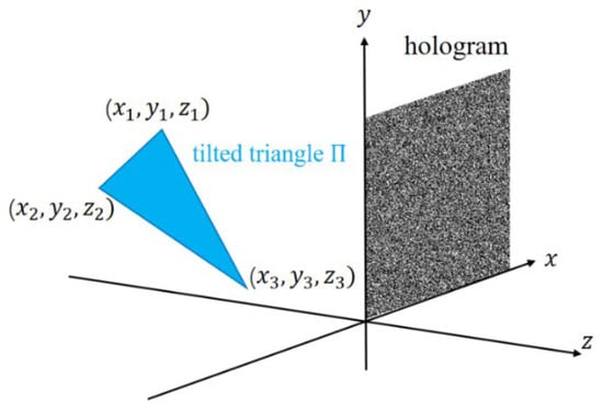
Figure 3.
Tilted triangle in global coordinate system and hologram plane
We now define the affine coordinates ) as our input coordinates, as shown in Figure 4. A primitive triangle with vertexes and is in the affine coordinate system, and the analytical expression of the primitive triangle spectrum is obtained by using two-dimensional Fourier transform for . The spectrum of the tilted triangle is finally obtained from the affine relationship between the primitive triangle and the tilted triangle with the analytical expression of the primitive triangle spectrum derived from the Fourier transform.
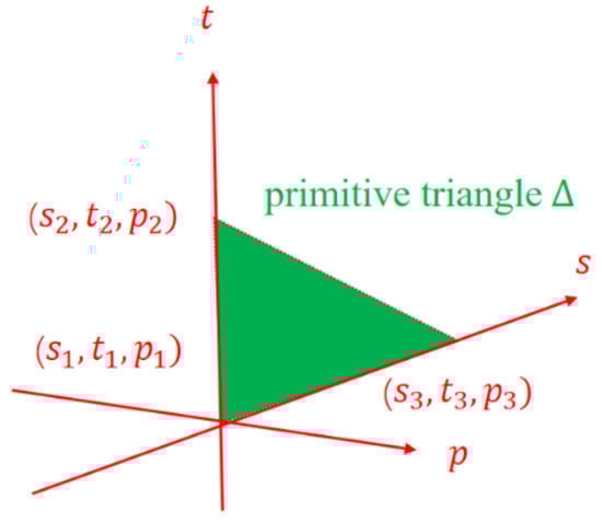
Figure 4.
Primitive triangle in affine coordinate system .
Through affine transformation we can map affine coordinates into global (output) coordinates , where is the coordinate vector of tilted triangle in the global coordinate system, is the coordinate vector of primitive triangle in the affine coordinates and the superscript denotes the transpose operation. is a 3 × 3 matrix and is a 3 × 1 vector. We let =, = =. Therefore, we can write in terms of matrix multiplication as shown in Equation (6), where is the affine transformation matrix and and represent matrices consisting of vertexes of tilted triangle and primitive triangle , respectively. By calculating the twelve parameters of affine matrix , we can uniquely determine the 3D affine transformation:
The key to the affine transformation algorithm is to find the elements of affine matrix . There is no inverse for 4 × 3 matrix , because inverse only exists for square matrices. The affine matrix has been found by using the pseudo inverse matrix of []. The accurate method is to avoid the use of pseudo matrices and to find the affine transformation matrix through direct calculation of . There are twelve unknown elements in affine matrix , and so we have to solve twelve equations to get these twelve elements. However, each matrix and only contain three vertexes in Equation (6). From this, we can only get nine equations to solve for the nine elements; the remaining elements in the affine matrix cannot be determined. In light of this, we introduce a new set of vertexes in matrix and a 4 × 1 vector in matrix to determine all the unknown twelve elements of the affine matrix . Therefore, we extend and to a matrix and , respectively. In light of this, Equation (6) becomes:
In order to simplify calculations and improve the calculation efficiency, the best choice is let and =. Then, becomes
Through simple calculations, we can obtain , indicating the existence of the inverse matrix of Then, we can find the affine transformation matrix by . Note that the vertex only represents a point located in the primitive coordinate system independent of the primitive triangle, and the value of and must be chosen such that to make sure the inverse of exists. can take any value; different values of make a different affine transformation matrix and the Jacobian determinant also changes at the same time. Again, we have chosen Equation (8) for ease of calculations and there is no effect on the final results that we end up solving. According to the above discussion, the affine transformation matrix can be obtained by Equation (7):
For primitive triangle , assuming that its surface function has strength of one within the triangle and zero outside, its spectrum analytical expression can be obtained (see Appendix A):
where are the spatial frequencies corresponding to affine coordinates and . The singular points , or have been discussed in Appendix A. Through affine transformation, the spectrum distribution of tilted triangle on the hologram plane is (see the derivation of this equation in Appendix B):
where again are spatial frequencies of the global coordinate system, is the surface function of the tilted triangle =, = and the Jacobian determinant . Then, the spectrum distribution on the hologram is:
which has been derived in Appendix C. Note that for an arbitrary tilted polygon, we can set an arbitrary point instead of point of the polygon. For a different choice, it will change the affine transform matrix, but the Jacobian determinant in Equation (12) also changes at the same time, giving the same result in Equation (12).
As shown in Figure 5a, the zero frequency in the global coordinate system is . According to the spatial frequency relationship given by Equation (28) in Appendix C, as shown in Figure 5b, the zero frequency in the affine coordinate system is :
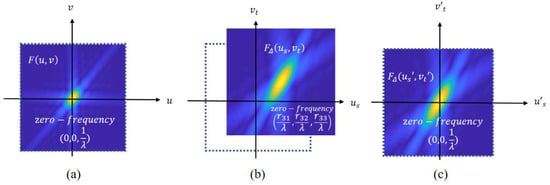
Figure 5.
Spectrum shift problem. (a) Spectrum in global coordinate system, (b) spectrum in affine system and (c) spectrum with frequency offsetting.
From the above equation, we can see that the zero frequency in the affine coordinate system has a frequency offset, and this offset will be represented in the reconstruction image with a phase factor. To eliminate this offset, as shown in Figure 5c, we can subtract this frequency offset according to
where Therefore, the spatial frequencies in the “offset” affine coordinate system can be rewritten as
The spectrum of a tilted triangle on the hologram plane now has been completely analyzed, and we can directly obtain the spectrum distribution through the initial parameters. For a single tilted triangle, we have as in Equation (2), and for a 3D object we use Equation (1). The complex field distribution of a 3D object reconstructed by the hologram can be expressed as the superposition of a tilted triangle complex field on reconstructed image plane :
where is the distance between the reconstructed image plane and the hologram plane . Through the above steps, we can obtain the reconstructed complex field distribution of the 3D object through only one Fourier transform. In the next section, we will verify our proposed method through numerical simulations and optical experiments.
4. Simulations and Optical Experiment
4.1. Numerical Reconstruction
Based on the 3D mesh in Figure 1, the Stanford bunny consists of 59,996 polygons, and we have reconstructed the bunny using our proposed method. The actual size of the bunny was 3.11 × 3.08 × 2.41 mm3. We have increased its size to 6.56 × 6.49 × 5.08 mm3 before the generation of the hologram. In order to improve the computational efficiency and image quality, we have implemented back-face culling by judging normal. The normal vector of a hologram is , and is the normal vector of a tilted triangle. If , the tilted triangle will be calculated, and tilted triangles that do not meet the condition will be discarded.
After back-face culling, the bunny only contains 31,724 polygons. However, in Section 3 the result of Equation (12) is based on the assumption that the amplitude distribution of a triangle is a unit constant and the reconstructed results will lack realism. As shown in Figure 6, in order to reproduce the details of the 3D object, we assign the surface function of the tilted triangle as follows:
where are the components of unit normal vector of the xyz-axis in the global coordinate system, and represents ambient reflected light. , and are the direction cosine values of illumination directions. In our case, .
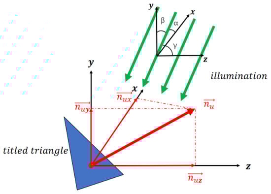
Figure 6.
Principle of flat shading.
The surface function usually refers to the strength information, and the amplitude is expressed as The surface function of the titled triangle is a constant for each tilted triangle according to Equation (17), so that we can let (I is a constant here) and by using the property of Fourier transform: the spectrum in the hologram of a tilted triangle with added flat shading and the elimination of the “offset” is based on Equation (12), together with Equation (15), we have:
Figure 7 shows the numerical reconstructions of the bunny based on our proposed F3DAAT method. Figure 7a is the result of calculating Equation (12), and we can see that because the amplitude of each mesh is the same constant the reconstruction result is a lack of realism. Additionally, the bunny has self-occlusion, so that back-face culling by judging normal will have some errors for some polygons. Due to the wrong judgment, visible polygons and invisible polygons are superimposed together and the reconstructed part of the image is shown in the red box on Figure 7a. Figure 7b,c are the reconstruction results based on Equation (18), and from these two reconstructed images we can clearly see the details of various parts of the bunny. Figure 7b focuses on the bunny’s leg, shown in the yellow box, and Figure 7c focuses on the bunny’s ear, shown in the yellow box.
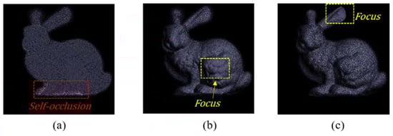
Figure 7.
Numerical reconstruction of the bunny. (a) Focus on leg without shading, (b) focus on leg with shading, (c) focus on ear with shading.
We have also scanned a human face called “Alex” with a 3D camera, and the 3D mesh of “Alex” is shown in Figure 8a, which consists of 49,272 meshes. In this case, there is no need to use back-face culling, because the data is the result from actual image scanning. We have calculated the CGH of “Alex”, and its holographic reconstructed image is shown in Figure 8b.
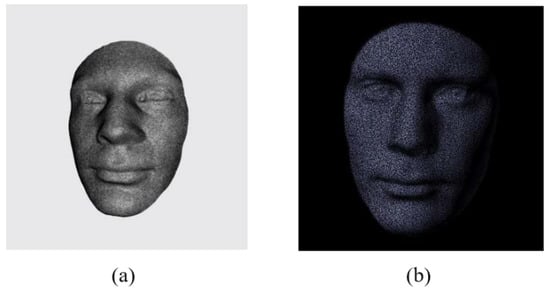
Figure 8.
Numerical reconstruction of “Alex”: (a) 3D mesh of Alex and (b) numerical reconstruction. The geometric surface with the texture image in (a) is from a publicly accessible geometric archive from the 3D Scanning Laboratory in Stony Brook University [].
4.2. Comparison with Previous Methods
The Pseudo Inverse Matrix Method by Pan et al. [,] sets up an affine transformation matrix that contains all the information on the transformation. However, they have defined the primitive triangle located at , i.e., the plane of the source local coordinate system, leading to the concept of a pseudo inverse matrix to perform matrix inversion. The introduction of the pseudo inverse matrix has produced calculation errors and slowed down the calculation speed. Zhang et al. [] have introduced a Full Analytical 3D Affine Method to avoid the use of the pseudo inverse matrix. The method includes three core steps: rotation transformation for the tilted triangle until it is parallel to the hologram plane, 2D affine transform of the rotated triangle and finally the computation of the field distribution on the hologram by using the angular spectrum (AS) method for diffraction. Zhang et al. [] also have proposed a Fast 3-D Affine Transformation (F3DAT) method based on the 3D affine transformation by Pan et al., to improve the computation efficiency. In the method, they have defined the primitive triangle located at , allowing the affine matrix to be fully inverted. The result of the F3DAT method provides a faster calculation time compared with that of the pseudo inverse matrix method and full analytical 3D affine method.
In the present proposed fast 3D analytical affine transformation (F3DAAT) method, we have obtained the affine matrix directly and derived an analytical expression of the spectrum of the primitive triangle. The more meshes that are calculated the more time F3DAAT will save. We have generated the holograms with a resolution of 1024 × 1024, and the hardware includes Intel Core i7-11700 @ 4.8GHz, 16G-byte RAM under the environment of MATLAB 2018b.
The Stanford bunny consisting of 31,724 meshes (after back-face culling) takes 893 s for the calculation, and the calculation of “Alex” of 49,272 meshes takes about 1288 s (See Figure 9). Additionally, shown in Figure 9 where we have used “Alex”, we can see that the computational efficiency of F3DAAT has increased by almost two times compared with the previous methods. The calculation of the four methods is based on the same hardware condition and only CPU is used for the calculation. In one of the most recent studies, Wang et al. [] proposed a polygon-based method using LUTs (look-up tables) with principal component analysis to speed up the calculation of CGHs. However, the method in the process of pre-computing the affine matrix still needs to solve a pseudo inverse matrix, and our proposed method is more general and efficient for solving the mapping relationship between the two coordinate systems, the global and the affine coordinate systems.
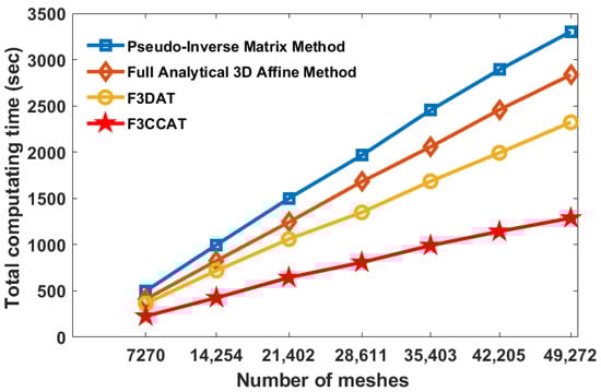
Figure 9.
Computation time required for different number of meshes for different methods for “Alex”.
4.3. Optical Experiment
The optical experiment is shown in Figure 10. We have reconstructed 3D objects by loading the phase of the CGHs from the computer onto the spatial light modulator (SLM). The SLM in our experiment is a HOLOEYE PLUTO2 (NIR-011) phase-only SLM with a resolution of 1920 × 1080 (Full HD 1080p) and a pixel pitch of 8 μm and the active area is 15.36 mm × 8.64 mm. The laser is a green light with a wavelength of 532 nm. The spatial filter is used to generate a collimated light for the illumination of the hologram. The polarizer is for adjusting the polarization state of the light to work with the phase-only SLM. A camera (MMRY UC900C Charge-coupled Device) is used to receive the reconstructed image in the image plane of the imaging lens (focal length is 150 mm). Optical reconstructions of the bunny and the face of “Alex” are shown in Figure 11a,b, respectively.
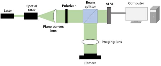
Figure 10.
Optical reconstruction experiment.
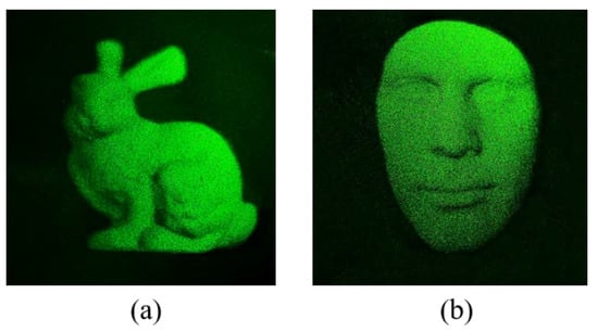
Figure 11.
Results of optical reconstruction: (a) bunny and (b) Alex.
5. Conclusions
In conclusion, we have proposed an improved algorithm to obtain a full-analytical spectrum of a tilted triangle based on 3D affine transformation. Our method avoids the time-consuming steps such as the need to solve for the pseudo inverse matrix or the complex process of 3D rotation and transformation. We have verified our method by calculating complex 3D objects composed of tens of thousands of meshes. In addition, we have added flat shading for realistic image presentation. We have successfully obtained the reconstructed images by numerical and optical reconstructions. Through comparison, it is found that our method improves the computational efficiency by about two times compared with the previous affine methods.
Author Contributions
Conceptualization, B.Z. and Y.Z.; formal analysis, Y.Z.; methodology, software, H.F., F.W.; investigation and validation, H.F., W.Q. and Q.F.; writing—original draft, H.F.; writing—review and editing, Y.Z. and T.-C.P. All authors have read and agreed to the published version of the manuscript.
Funding
This research was funded by National Natural Science Foundation of China (61865007) and Yunnan Provincial Science and Technology Department (2019FA025).
Data Availability Statement
Original data are available in Ref. [].
Acknowledgments
We appreciate the use of the SLM, which is on loan from Yanfei Lv, Department of Physics and Astronomy, Yunnan University. We would like to thank Pin Wang for her help with the first draft.
Conflicts of Interest
The authors declare no conflict of interest.
Appendix A. Full Results of the Analytical Spectrum Expression of Primitive Triangle
Case 1: when the integration result of Equation (10) is:
Case 2: when the integration result of Equation (10) is:
Case 3: when the integration result of Equation (10) is:
Case 4: when the integration result of Equation (10) is:
Case 5: when the integration result of Equation (10) is:
Appendix B. Derivation of the Spectrum Distribution of Tilted Triangle on the Hologram Plane
In Figure A1a, we show tilted triangle in the global coordinate system. In Figure A1b, we represent as a collection of discrete parallel planes . has a length of as shown in Figure A1b. The spectrum of can be expressed as = Therefore, the spectrum of in the hologram plane is = . Hence, the spectrum of in the hologram plane can be written as:
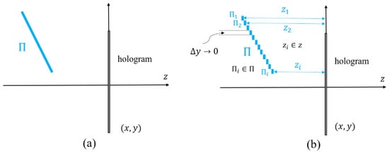
Figure A1.
(a) Tilted triangle in the global coordinate system, (b) discrete version of .
Now
where is the surface function of We put Equation (A7) into Equation (A6) to achieve:
where is the surface function of Equation (A8) is presented in Equation (11).
Appendix C. Derivation of the Analytical Spectrum Expression of Tilted Triangle on the Hologram
According to affine transformation, . Therefore, the coordinate relationships between the global coordinate system and affine coordinate system are:
Additionally, the relationships between the spatial frequencies of the global coordinate system and the affine coordinate system are . We can write as follows:
Note, that we have chosen , by using Equations (A9) and (A10), the exponential term in Equation (11) can be rewritten as:
In Equation (A11), we have used the elements in the affine matrix already solved in Equation (9), i.e., Then, according to Equations (11) and (A11), the analytical spectrum of the tilted triangle can be rewritten as:
which is presented in Equation (12).
References
- Jason, G. Three-dimensional display technologies. Adv. Opt. Photonics 2013, 5, 456–535. [Google Scholar]
- Liu, L.; Pang, L.; Teng, D. Super multi-view three-dimensional display technique for portable devices. Opt. Express 2016, 24, 4421–4430. [Google Scholar] [CrossRef] [PubMed]
- Hoffman, D.; Girshick, A.; Akeley, K.; Banks, M. Vergence-accommodation conflicts hinder visual performance and cause visual fatigue. J. Vis. 2008, 8, 1–30. [Google Scholar] [CrossRef]
- Smalley, D.; Nygaard, E.; Squire, K.; Wagoner, J.; Rasmussen, J.; Gneiting, S.; Qaderi, K.; Goodsell, J.; Rogers, W.; Lindsey, M. A photophoretic-trap volumetric display. Nature 2018, 553, 486–490. [Google Scholar] [CrossRef]
- Jung, J.; Kim, J.; Lee, B. Solution of pseudoscopic problem in integral imaging for real-time processing. Opt. Lett. 2013, 38, 76–78. [Google Scholar] [CrossRef]
- Poon, T.-C.; Liu, J.-P. Introduction to Modern Digital Holography with MATLAB; Cambridge University Press: Cambridge, UK, 2014. [Google Scholar]
- Matsushima, K. Introduction to Computer Holography; Springer: New York, NY, USA, 2020; pp. 54–88. [Google Scholar]
- Zhang, Y.; Fan, H.-X.; Wang, F.; Gu, F.; Qian, X.; Poon, T.-C. Polygon-based computer-generated holography: A review of fundamentals and recent progress [Invited]. Appl. Opt. 2021, 61, B363–B374. [Google Scholar] [CrossRef]
- Wang, Z.; Lv, G.; Feng, Q.; Wang, A.; Ming, G. Resolution Priority Holographic Stereogram Based on Integral Imaging with Enhanced Depth Range. Opt. Express 2019, 27, 2689–2702. [Google Scholar] [CrossRef]
- Zhang, X.; Lv, G.; Wang, Z.; Hu, Z.; Ding, S.; Feng, Q. Resolution-Enhanced Holographic Stereogram Based on Integral Imaging Using an Intermediate-View Synthesis Technique. Opt. Commun. 2020, 457, 124656. [Google Scholar] [CrossRef]
- Nishitsuji, T.; Yamamoto, Y.; Takashige, S.; Takanori, A.; Hirayama, R.; Nakayama, H.; Kakue, T.; Shimobaba, T.; Ito, T. Special-purpose computer HORN-8 for phase-type electro-holography. Opt. Express 2018, 26, 26722–26733. [Google Scholar] [CrossRef]
- Zhao, Y.; Cao, L.; Zhang, H.; Kong, D.; Jin, G. Accurate calculation of computer-generated holograms using angular-spectrum layer-oriented method. Opt. Express 2015, 23, 25440–25449. [Google Scholar] [CrossRef]
- Nishitsuji, T.; Shimobaba, T.; Kakue, T.; Ito, T. Review of fast calculation techniques for computer-generated holograms with the point-light-source-based model. IEEE Trans. Ind. Inform. 2017, 13, 2447–2454. [Google Scholar] [CrossRef]
- Lucente, M. Interactive computation of holograms using a look-up table. J. Electron. Imaging 1993, 2, 28–34. [Google Scholar] [CrossRef]
- Kim, S.; Kim, E. Fast computation of hologram patterns of a 3D object using run-length encoding and novel look-up table methods. Appl. Opt. 2009, 48, 1030–1041. [Google Scholar] [CrossRef]
- Pan, Y.; Xu, X.; Solanki, S.; Liang, X.; Tanjung, R.; Tan, C.; Chong, T. Fast CGH computation using S-LUT on GPU. Opt. Express 2009, 17, 18543–18555. [Google Scholar] [CrossRef]
- Shimobaba, T.; Ito, T.; Masuda, N.; Ichihashi, Y.; Takada, T. Fast calculation of computer-generated-hologram on AMD HD5000 series GPU and OpenCL. Opt. Express 2010, 18, 9955–9960. [Google Scholar] [CrossRef] [PubMed] [Green Version]
- Ichihashi, Y.; Oi, R.; Senoh, T.; Yamamoto, K.; Kurita, T. Real-time capture and reconstruction system with multiple GPUs for a 3D live scene by a generation from 4K IP images to 8K holograms. Opt. Express 2012, 20, 21645–21655. [Google Scholar] [CrossRef] [PubMed]
- Leseberg, D.; Frère, C. Computer-generated holograms of 3-D objects composed of tilted planar segments. Appl. Opt. 1988, 27, 3020–3024. [Google Scholar] [CrossRef]
- Matsushima, K. Formulation of the rotational transformation of wave fields and their application to digital holography. Appl. Opt. 2008, 47, D110–D116. [Google Scholar] [CrossRef] [Green Version]
- Matsushima, K.; Schimmel, H.; Wyrowski, F. Fast calculation method for optical diffraction on tilted planes by use of the angular spectrum of plane waves. J. Opt. Soc. Am. A 2003, 20, 1755–1762. [Google Scholar] [CrossRef]
- Matsushima, K. Computer-generated holograms for three-dimensional surface objects with shade and texture. Appl. Opt. 2005, 44, 4607–4614. [Google Scholar] [CrossRef] [PubMed]
- Ahrenberg, L.; Benzie, P.; Magnor, M.; Watson, M. Computer generated holograms from three dimensional meshes using an analytic light transport model. Appl. Opt. 2008, 47, 1567–1574. [Google Scholar] [CrossRef] [PubMed]
- Kim, H.; Hahn, J.; Lee, B. Mathematical modeling of triangle-mesh-modeled three-dimensional surface objects for digital holography. Appl. Opt. 2008, 47, D117–D127. [Google Scholar] [CrossRef] [PubMed] [Green Version]
- Pan, Y.; Wang, Y.; Liu, J.; Li, X.; Jia, J. Fast polygon-based method for calculating computer-generated holograms in three-dimensional display. Appl. Opt. 2013, 52, A290–A299. [Google Scholar] [CrossRef]
- Pan, Y.; Wang, Y.; Liu, J.; Li, X.; Jia, J. Improved full analytical polygon-based method using Fourier analysis of the three-dimensional affine transformation. Appl. Opt. 2014, 53, 1354–1362. [Google Scholar] [CrossRef]
- Zhang, Y.; Zhang, J.; Chen, W.; Zhang, J.; Wang, P.; Xu, W. Research on three-dimensional computer-generated holographic algorithm based on conformal geometry theory. Opt. Commun. 2013, 309, 196–200. [Google Scholar] [CrossRef]
- Zhang, Y.; Zhang, J.; Chen, W.; Wang, P.; Wu, S.; Li, J. Fast Computer-generated Hologram Algorithm of Triangle Mesh Models. Chin. J. Lasers 2013, 40, 0709001. [Google Scholar] [CrossRef]
- Zhang, Y.-P.; Wang, F.; Poon, T.-C.; Fan, S.; Xu, W. Fast generation of full analytical polygon-based computer-generated holograms. Opt. Express 2018, 26, 19206–19224. [Google Scholar] [CrossRef]
- Matsushima, K. Performance of the Polygon-Source Method for Creating Computer-Generated Holograms of Surface Objects. In Proceedings of the ICO Topical Meeting on Optoinformatics/Information Photonics, Petersburg, Russia, 4–7 September 2006. [Google Scholar]
- Bracewell, R.; Chang, K.; Jha, A.; Wang, Y. Affine theorem for two-dimensional Fourier transform. Electron. Lett. 1993, 29, 304. [Google Scholar] [CrossRef]
- Underkoffler, J. Occlusion Processing and Smooth Surface Shading for Fully Computed Synthetic Holography. In Proceedings of the Practical Holography XI and Holographic Materials III, San Jose, CA, USA, 8 February 1997. [Google Scholar]
- Gilles, A.; Gioia, P. Real-time layer-based computer-generated hologram calculation for the Fourier transform optical system. Appl. Opt. 2018, 57, 8508–8517. [Google Scholar] [CrossRef]
- Zhang, H.; Cao, L.; Jin, G. Computer-generated hologram with occlusion effect using layer-based processing. Appl. Opt. 2017, 56, F138–F143. [Google Scholar] [CrossRef]
- Frère, C.; Leseberg, D.; Bryngdahl, O. Computer-generated holograms of three-dimensional objects composed of line segments. J. Opt. Soc. Am. A 1986, 3, 726–730. [Google Scholar] [CrossRef]
- Lee, W.; Im, D.; Paek, J.; Hahn, J.; Kim, H. Semi-analytic texturing algorithm for polygon computer-generated holograms. Opt. Express 2014, 22, 31180–31191. [Google Scholar] [CrossRef] [PubMed]
- Ji, Y.; Yeom, H.; Park, J. Efficient texture mapping by adaptive mesh division in mesh-based computer generated hologram. Opt. Express 2016, 24, 28154–28169. [Google Scholar] [CrossRef] [PubMed]
- Yamaguchi, K.; Ichikawa, T.; Sakamoto, Y. Calculation method for CGH considering smooth shading with polygon models. Proc. SPIE 2011, 7957, 795706. [Google Scholar]
- Matsushima, K.; Sonobe, N. Full-color digitized holography for large-scale holographic 3D imaging of physical and nonphysical objects. Appl. Opt. 2018, 57, A150–A156. [Google Scholar] [CrossRef]
- Matsushima, K.; Nakahara, S. Extremely high-definition full-parallax computer-generated hologram created by the polygon-based method. Appl. Opt. 2009, 48, H54–H63. [Google Scholar] [CrossRef]
- Matsushima, K.; Nakamura, M.; Nakahara, S. Silhouette method for hidden surface removal in computer holography and its acceleration using the switch-back technique. Opt. Express 2014, 22, 24450–24465. [Google Scholar] [CrossRef]
- Stony Brook University 3D Scanning Laboratory. Available online: https://www3.cs.stonybrook.edu/~gu/software/holoimage/index.html (accessed on 4 July 2022).
- Wang, F.; Shimobaba, T.; Zhang, Y.; Kakue, T.; Ito, T. Acceleration of polygon-based computer-generated holograms using look-up tables and reduction of the table size via principal component analysis. Opt. Express 2021, 29, 35442–35455. [Google Scholar] [CrossRef]
Publisher’s Note: MDPI stays neutral with regard to jurisdictional claims in published maps and institutional affiliations. |
© 2022 by the authors. Licensee MDPI, Basel, Switzerland. This article is an open access article distributed under the terms and conditions of the Creative Commons Attribution (CC BY) license (https://creativecommons.org/licenses/by/4.0/).