Article

Integration of Hydrological Model and Time Series Model for Improving the Runoff Simulation: A Case Study on BTOP Model in Zhou River Basin, China

1
State Key Laboratory of Hydraulics and Mountain River Engineering, College of Water Resource and Hydropower, Sichuan University, No. 24 South Section 1, Yihuan Road, Chengdu 610065, China
2
Institute for Disaster Management and Reconstruction, Sichuan University-Hong Kong Polytechnic University, Chengdu 610065, China
3
College of Water Resources and Hydropower, Sichuan Agricultural University, Ya’an 625014, China
*
Authors to whom correspondence should be addressed.
Appl. Sci. 2022, 12(14), 6883; https://doi.org/10.3390/app12146883
Submission received: 11 May 2022 / Revised: 28 June 2022 / Accepted: 5 July 2022 / Published: 7 July 2022
(This article belongs to the Section Earth Sciences)

Abstract

:

Featured Application

The application provides a new tool for reducing the error in the simulated runoff of a hydro-logical model by integrating time series models with hydrological models.

Abstract

Improving the accuracy of runoff simulations is a significant focus of hydrological science for multiple purposes such as water resources management, flood and drought prediction, and water environment protection. However, the simulated runoff has limitations that cannot be eliminated. This paper proposes a method that integrates the hydrological and time series models to improve the reliability and accuracy of simulated runoffs. Specifically, the block-wise use of TOPMODEL (BTOP) is integrated with three time series models to improve the simulated runoff from a hydrological model of the Zhou River Basin, China. Unlike most previous research that has not addressed the influence of runoff patterns while correcting the runoff, this study manually adds the hydrologic cycle to the machine learning-based time series model. This also incorporates scenario-specific knowledge from the researcher’s area of expertise into the prediction model. The results show that the improved Prophet model proposed in this study, that is, by adjusting its holiday function to a flow function, significantly improved the Nash–Sutcliffe efficiency (NSE) of the simulated runoff by 53.47% (highest) and 23.93% (average). The autoregressive integrated moving average (ARIMA) model and long short-term memory (LSTM) improved the runoff but performed less well than the improved Prophet model. This paper presents an effective method to improve the runoff simulation by integrating the hydrological and time series models.

1. Introduction

Runoff simulation is one of the most important topics in current surface hydrological process research [1]. Runoff is an essential link in the process of the surface water cycle, and is an important indicator that reflects the resource and environmental conditions of the basin. Its changes objectively reflect the changes in regional hydrological processes and water resources’ inventory [2,3]. The hydrological model is an excellent instrument for runoff simulation, analysis, and calculation, and it is a crucial way to explore and understand the water cycle and hydrological processes. The hydrological model also simulates the main characteristics of the rainfall-runoff process by generalizing the complex water cycle process, which is important for water resources development and utilization, flood prevention and mitigation, urban planning, vegetation impacts and watershed response to human activities, and many other aspects [4,5,6,7]. With the wide application of hydrological models, the issue of how to improve the accuracy of rainfall-runoff simulations has attracted more and more attention from scholars and has increasingly become one of the critical topics in hydrology research [4].
Modern time series analysis originated in 1927 with the autoregressive (AR) model proposed by the British statistician Yule [8]. Together with the moving average (MA) model and the ARMA model proposed by Walker in 1931, this model formed the basis of time series analysis and is still heavily used today [9]. With the continuous development of the theory and application of time series analysis, time series models are used in many fields such as finance, e-commerce, information and data mining. The common time series models include: (1) autoregressive (AR) models, moving average (MA) models, and autoregressive integrated moving average (ARIMA) models based on traditional probabilistic statistical methods [10]; (2) the BP neural network model and long and short-term memory (LSTM) neural network models based on machine learning algorithms [11,12]; and (3) the Prophet model based on time series decomposition and machine learning fitting.
The use of error correction models to improve the accuracy of hydrological model forecasts is an effective tool [13], and time series models have also played a significant role in this regard. Montanari et al. [14] used the meta-Gaussian model to predict the posterior distribution of errors to obtain the predicted flow interval results with a certain confidence. Cheng et al. [15] employed the ARMA-GARCH model with the heteroscedasticity of the hydrological sequence to post-process the error series of runoff simulated by the Xinanjiang model to obtain real-time flood prediction results, which significantly improved the prediction accuracy. Zhang et al. [16] applied the Bayesian forecasting system (BFS) and hydrologic uncertainty processor (HUP) to the Baishan Reservoir basin to obtain a posterior distribution of predicted flow to reduce simulation uncertainty. Jiao et al. [17] took the Shuibuya upstream watershed as the study area and established the regression model of distributed hydrological model DEM-based distributed rainfall-runoff model (DDRM) simulation results for the real-time correction of the runoff simulation. The results show that the regression model, to a certain extent, makes up for the actual application of distributed hydrological model due to lack of information and the decline in precision. Qu et al. [13] used two real-time correction technologies, the autoregressive (AR) model and the entire-process joint correction method (EPJC), to predict and correct the runoff error of the Xinanjiang model in order to reduce the runoff prediction error in the Dadu River Basin, thus improving the actual forecasting ability of the hydrological model.
Time series models are used to correct the results of hydrological model predictions or simulations, and most of the existing methods are based on the principles of mathematical statistics or machine learning for model correction. This study adds a manual operation component to the time series prediction model based on the machine learning principle, and it is combined with the runoff model scheme of the hydrological model. The correction effect is significantly improved compared with the existing time series model correction methods. This study employs the improved Prophet, a time series model established by Facebook in 2017, combined with a distributed hydrological model, block-wise use of TOPMODEL (BTOP), and takes the ARIMA model and LSTM model as comparison models to demonstrate, in detail, the time series model’s prediction and analysis of error series of the distributed hydrological model. This provides a valuable reference for applying the time series model in hydrological model research.

2. Study Area and Data

2.1. Study Area

The study area comprises the Xuanhan section of the Zhou River, located in the southwestern part of Xuanhan County, Sichuan Province, China. The Zhou River is a first-class tributary of the Qu River, with the upper source divided into three branches: the front, middle and back rivers. The front river is the mainstream, with all originating from the southern foot of the Daba Mountains and flowing in a sinuous manner to the southwest (Figure 1). The Qu River is an important tributary of the Jialing River, with sufficient water supply, large flood and dry variability, and a relatively obvious runoff pattern. Its runoff series is suitable for use as the time series data for this study.
The basin area of the study area is 3574 km2, the mainstream length is about 108 km, the river bed width is about 60 m, the natural drop is 16.6–327 m, the average annual flow is 160 m3/s, the annual average temperature is 16.7 °C, and the annual average rainfall is 1230 mm, with the majority of it falling between May and October, accounting for roughly 70% of the total. There are 6 soil types, and 106 variants in the study basin, and the main soil types are purple soil, rice soil and loam. The study basin is influenced by the southwest monsoon, with abundant precipitation and frequent floods, including the historical floods in 1902, 1982 and 2004. Floods in this area are closely related to climatic precipitation, so it is important to simulate rainfall-runoff in the study area.

2.2. Data

The years from 1982 to 1984 were selected as the training period and 1985 was chosen as the testing period for the study. Twenty-one rainfall stations and four flow stations (in the locations of Donglin, Tuhuang, Qingxi, and Maoba) were selected within the study basin. The daily precipitation data and daily flow data were derived from the hydrology Yearbook published by the Hydrology Bureau of the Ministry of Water Resources of China. Terrain data were derived from digital elevation model (DEM) data with 30 m resolution provided by a geospatial data cloud [18]. Land use/vegetation cover type data obtained at 500 m grid scale were from USGS Land Cover Research Institute [19]. Soil data from the Food and Agriculture Organization of the United Nations (FAO) provided a global 1:5 million proportion of raster data [20]. The potential interception of reservoir (PET0) evaporation data with a 0.25-degree resolution were obtained from the Global Terrestrial Evaporation Amsterdam model (GLEAM) [21]. The potential evapotranspiration (EP) data were obtained from the Climate Research Unit (CRU) with a resolution of 0.5 degrees [22]. Leaf area index (LAI) data with a resolution of 0.05 degrees were adopted from the National Environmental Information Center (NCEI) [23]. All the above data sets were resampled to 1 km and input into the BTOP model for runoff simulation [24].

3. Methodology

3.1. Hydrological Model: The Block-Wise Use of TOPMODEL (BTOP Model)

The BTOP model is a distributed watershed hydrological model based on a physical mechanism [25,26]. It was initially developed at Yamanashi University, Japan [27] for distributed hydrological simulation of large basins [28].
Compared with the traditional TOPMODEL model, the BTOP model was developed based on its in-depth analysis and improvement. It has made some progress in terms of river network technology, natural sub-basin delineation, the method of giving the spatial distribution of the catchment model parameters as grid cells, and confluence accuracy [29]. The BTOP model has been widely used in the hydrological simulation of various river basins worldwide, such as the Fuji River Basin [29,30,31] (3500 km2) in Japan, the Mekong River Basin [32,33] (811,000 km2), the Min River Basin in China [34], eight basins in Nepal [35] and a dozen small- and medium-sized watersheds in the United States [36]. Effective testing has been completed in all these river basins.
(1)
Runoff generation process
The BTOP model uses TOPMODEL as the runoff generation sub-model, and the raster cells are divided into four parts in the vertical direction: vegetation part, root part, unsaturated part and saturated part. The vegetation part includes rainfall and evapotranspiration processes, the unsaturated part is divided into active and inactive zones, and the lowermost layer is the saturated zone. The main flow generation types of grid cells include super permeability, full storage and base flow.
(2)
Flow routing process
The BTOP model uses the Muskingum–Cunge method as a flow routing sub-model, as a physically-based flow routing method rather than an empirical approach, this algorithm is equivalent to the convection-diffusion model and it is more suitable for large river basins than the kinematic wave model since the riverbed slopes are often mild.
(3)
Model parameters
The five calibration parameters for saturated transmissivity of soil are the block-average Manning coefficient ( n 0 c ), drying function parameter ( α ), discharge decay factor ( m ), block-average saturation deficit ( S D b a r ), and groundwater dischargeability ( D o ), which are used as the initial values in the training period of the model. They are automatically optimized by the SCE-UA [37] algorithm to obtain the parameters for the testing period, which are then substituted in the model for runoff simulation. The BTOP model was chosen because of its solid physical basis and few rate-determining parameters. Moreover, the parameters of the model all have physical meaning or interpretation for characterizing soil properties, land use and other features, which can effectively reduce the uncertainty of the model. Moreover, the model has a good application background in the Yangtze River basin, where the study area is located.

3.2. Autoregressive Integrated Moving Average Model (ARIMA Model)

The autoregressive integrated moving average (ARIMA) model is a time series forecasting analysis method [38]. ARIMA (p, d, q), in which AR is “autoregressive”, and p is the number of autoregressive terms. MA is the “sliding average”, q is the number of sliding average terms, and d is the number of differences to make it a stationary series [10]. In practice, d is usually less than 2, and is the key step to make the series smooth.
(1)
Autoregressive (AR) model
Under the condition that the time series satisfies smoothness, the AR model describes the treatment of the relationship between current and historical values, that is, to use the historical time data of the variable itself to predict itself [39]. The formula defines the P-order autoregressive process:
y t = μ + Σ i = 1 P γ i y t 1 + ε t
where y t is the simulation error at time t; μ is the constant term; P is the lag order of the autoregressive process; γ i is the autocorrelation coefficient; ε t is the random perturbation term.
(2)
Moving average (MA) model
The MA model is concerned with the accumulation of the error term in the AR model, that is, the error term ε t in the AR model is viewed as a moving average term of order q [40]. The autoregressive process of order q is defined by the formula:
y t = μ + ε t + Σ i = 1 q θ i ε t 1
where   y t is the simulation error at time t; μ is the constant term; q is the lag order of the moving average process; θ i is the autocorrelation coefficient; ε t is the random perturbation term.
(3)
Autoregressive integrated moving average (ARIMA) model
The autoregression is combined with the moving average to obtain the ARIMA (p, d, q) model defined by the formula:
y t = μ + Σ i = 1 P γ i y t 1 + ε t + Σ i = 1 q θ i ε t 1
From the formula, we know that we only need to specify three parameters (p, d, q) when getting the ARIMA model, where d is the order and d = 1 is the first-order difference. p, q can be determined according to the partial autocorrelation function (PACF) and autocorrelation function (ACF) of sequences [41].

3.3. Long Short-Term Memory (LSTM)-Based Prediction

LSTM is a special type of recurrent neural network (RNN) first proposed by Hochreiter and Schmidhuber (1997) [42], which is mainly used to solve the problems of gradient disappearance and gradient explosion in the process of long sequence training [43]. To put it simply, compared with ordinary RNN, LSTM can learn long-term rules and has better learning ability in longer sequences.
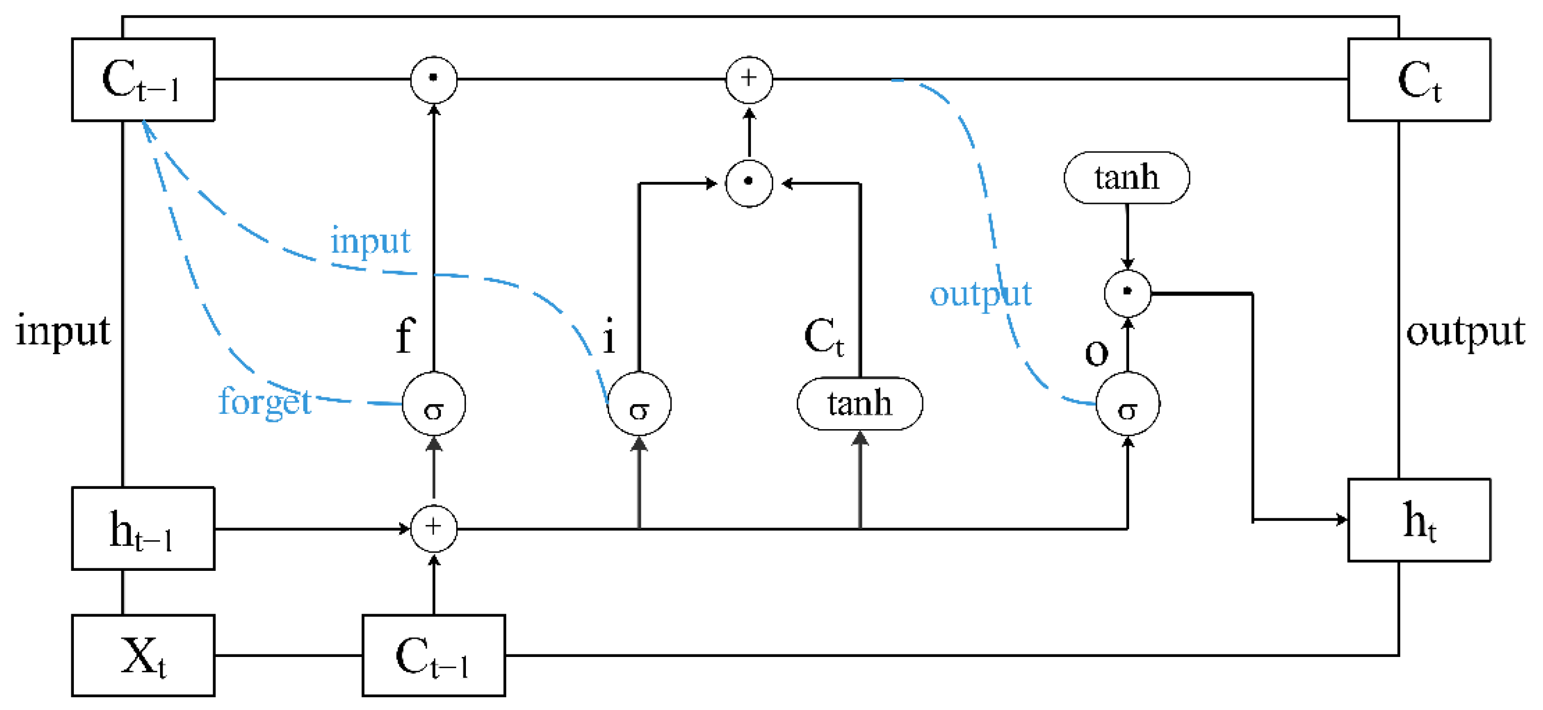
The chain structure of the LSTM contains three main gates, which are shown in Figure 2: (1) the forget gate f t , which determines how much of the cell state c t 1 from the previous moment is retained in the current cell state c t ; (2) the input gate i t , which determines how much of the input x t to the network is saved to the cell state c t at the current moment; and (3) the output gate o t , which controls the unit state c t and how many inputs it has to the current output value h t [44].
The forget gate determines what information is discarded from this node, and its main function is the Sigmoid, denoted by σ ; W f is the weight matrix; b f is the bias term. The formula is as follows:
f t = σ W f · h t 1 , x t + b f
The input gate selectively remembers the input information, and its primary function is similar to the forget gate. After the input, the candidate cell state can be combined with the forget gate and the input gate to c t ˜ to update the current moment cell state c t . The equation is as follows:
i t = σ W i · h t 1 , x t + b i
c t ˜ = tanh W c · h t 1 , x t + b c
c t = f t · c t 1 + i t · c t ˜
The output gate determines which will be retained as the current state output and combined with the current cell state to obtain the final output h t of the LSTM, the formula is as follows:
o t = σ W o · h t 1 , x t + b o
h t = o t · tanh c t

3.4. Improved Prophet Model

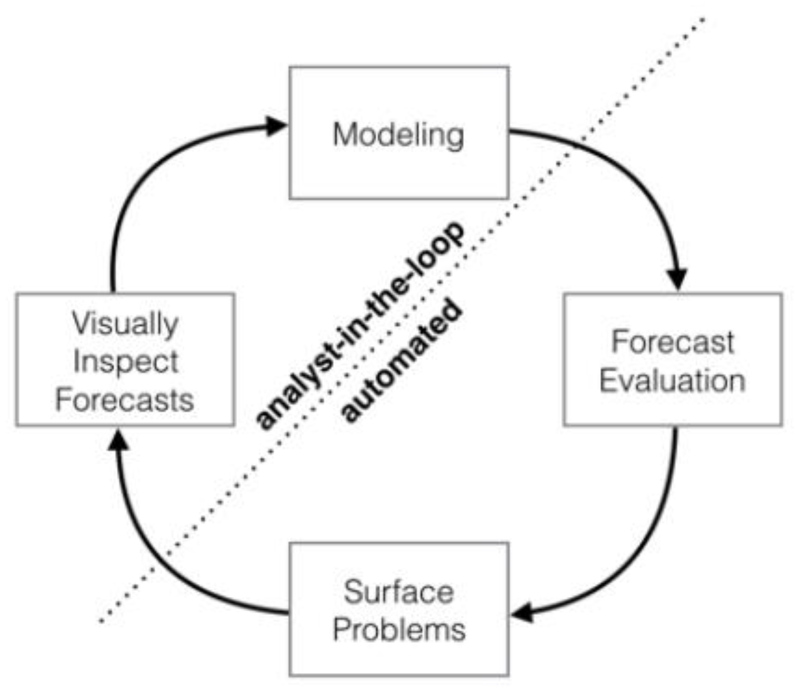
The Prophet model is a decomposable time series forecasting model open-sourced by Facebook [45,46]. The model is a whole-loop structure divided into a manual manipulation part and an automated part, which integrates background knowledge of specific problems and statistical analysis [46]. Analysts can check predictions and adjust models based on feedback and realistic scenarios. This combination makes the Prophet model more accurate and rapid, more automatic, and parameters are easier to adjust than the traditional time series prediction model [47]. The principle of the model is shown in Figure 3.
The algorithm of the model is formulated as follows:
Y t = g t + s t + f t + e t
which includes:
(1)
Trend function g t
This is the core part of the whole Prophet model, and is mainly used to represent the trend in the time series of the non-periodic changes. It reflects the overall trend in the fluctuation of the time series, while the future trend is predicted [48]. The trending term has two important functions: the segmented linear function based on linear regression, and the saturated growth function based on logistic regression. This simulation adopts a piecewise linear function [46].
(2)
Periodic function s t
The time series contains seasonal trends in various types of cycles, such as days, weeks, months and years [49]. For these irregular periodic variations, fitting these variations effectively has a significant effect on the accuracy of the model predictions. Therefore, the Prophet model approximates this cyclical property with a Fourier series [50].
(3)
Flow function f t
In the original Prophet model, this item is the holiday function h t . Prophet has built-in important holidays in each country, and in the prediction of the series affected by special time points such as sales volume or electricity consumption, the holiday term can effectively simulate the impact of special time points, such as a surge in orders on the National Day. As for the runoff error series in this study, it is not affected by holidays in the traditional sense. Through comparison and observation, it is found that the runoff error series is influenced by high-flow and low-flow periods, and the error in the BTOP simulation increases accordingly at the maximum point of runoff.
Therefore, the improved Prophet model uses the flow function f t to replace the original holiday function h t . The maximum value point in the runoff series is used as a special “holiday” to effectively reduce the effect of the high-flow periods on the error series, and the equation is as follows:
f t = Z t k = i = 1 L k i · L t D i
where k i denotes the influence range of the high flow periods, k follows a normal distribution, k ~ Normal 0 , q 2 . The parameter flow_prior_scale influences the normal distribution, and the parameter value is specified according to the average flow rate of each station. The larger the value, the greater the influence of the high-flow periods on the model; L is the number of extreme value points of the high-flow periods, and these points are located on the rainfall-runoff map and entered into the model by manually creating a data frame; D i indicates the date before and after the high-flow periods, and it is set using the lower_window and upper_window parameters, respectively.
(4)
White noise function e t
This function represents the residual fluctuation, and there is no specific formula for calculation. The mcmc_samples parameter was used to select the probability estimation mode. If the parameter is n (n > 0), the model will make a full Bayesian inference with n Markov sampling samples. In this paper, maximum posterior probability estimation (MAP) is directly adopted and the parameter is set to 0. This study uses the Python language under the Windows system to run the Prophet model, so the stan_backend parameter was set to cmdstanpy.
The debugging of the models is mostly automatic, which is an advantage that is common to many time series models [50]. What makes the Prophet model even better is that analysts can change the model in several places to apply their expertise and external knowledge [51], as in the case of this improved flow function f t . For the different average flow sizes of each hydrological station, the maximum value point in the f t during the high-flow periods is manually adjusted. Taking NSE as the main indicator, a set of parameters suitable for this analysis was finally obtained after several rounds of debugging and regular error sequence training. The Prophet model then accumulates the results of four parts as the predicted value of the time series.
Taking Donglin Station as an example, some parameters of the current Prophet model are shown in Table 1 after debugging.

3.5. Evaluation Indicators

In order to measure and detect the correction effects of the three time series models, the following five evaluation metrics are used in this study:
(1) Mean absolute error (MAE) is used to measure the average absolute error between the predicted value and the real value on the experimental data set. The smaller the value of MAE, the better the accuracy of the prediction model. For a test set containing n messages, MAE is defined as:
M A E = 1 n t = 1 n a c t u a l t f o r e c a s t t
(2) The root means square error (RMSE) is used to measure the deviation between the observed flow and the true value, which represents the expected value of the squared error and should also be as small as possible. RMSE is defined as follows:
R M S E = t = 1 n a c t u a l t f o r e c a s t t 2 n
(3) Average absolute percentage error (MAPE) is used to measure the relative errors between the average test value and the real value on the test set. The smaller the value of MAPE, the better the accuracy of the prediction model. MAPE is defined as:
M A P E = 1 n t = 1 n a c t u a l t f o r e c a s t t a c t u a l t × 100 %
(4) Pearson’s correlation coefficient R reflects the degree of linear correlation between two random variables. The closer r is to 0, the more linearly irrelevant the predicted and true values. The closer r is to 1, the more positively correlated the predicted and true values. With x, y representing a c t u a l t and f o r e c a s t t , respectively, R is defined as:
R = i = 1 n x i x ¯ y i y ¯ i = 1 n x i x ¯ 2 i = 1 n y i y ¯ 2
(5) The Nash–Sutcliffe efficiency coefficient (NSE) is generally used to verify the simulation results of the hydrological model, and the value of NSE range is ~ 1 ; the closer to 1, the better the simulation effect. NSE is defined as:
N S E = 1 t = 1 T Q 0 t Q m t 2 t = 1 T Q 0 t Q 0 ¯ 2

3.6. Methodology Structure

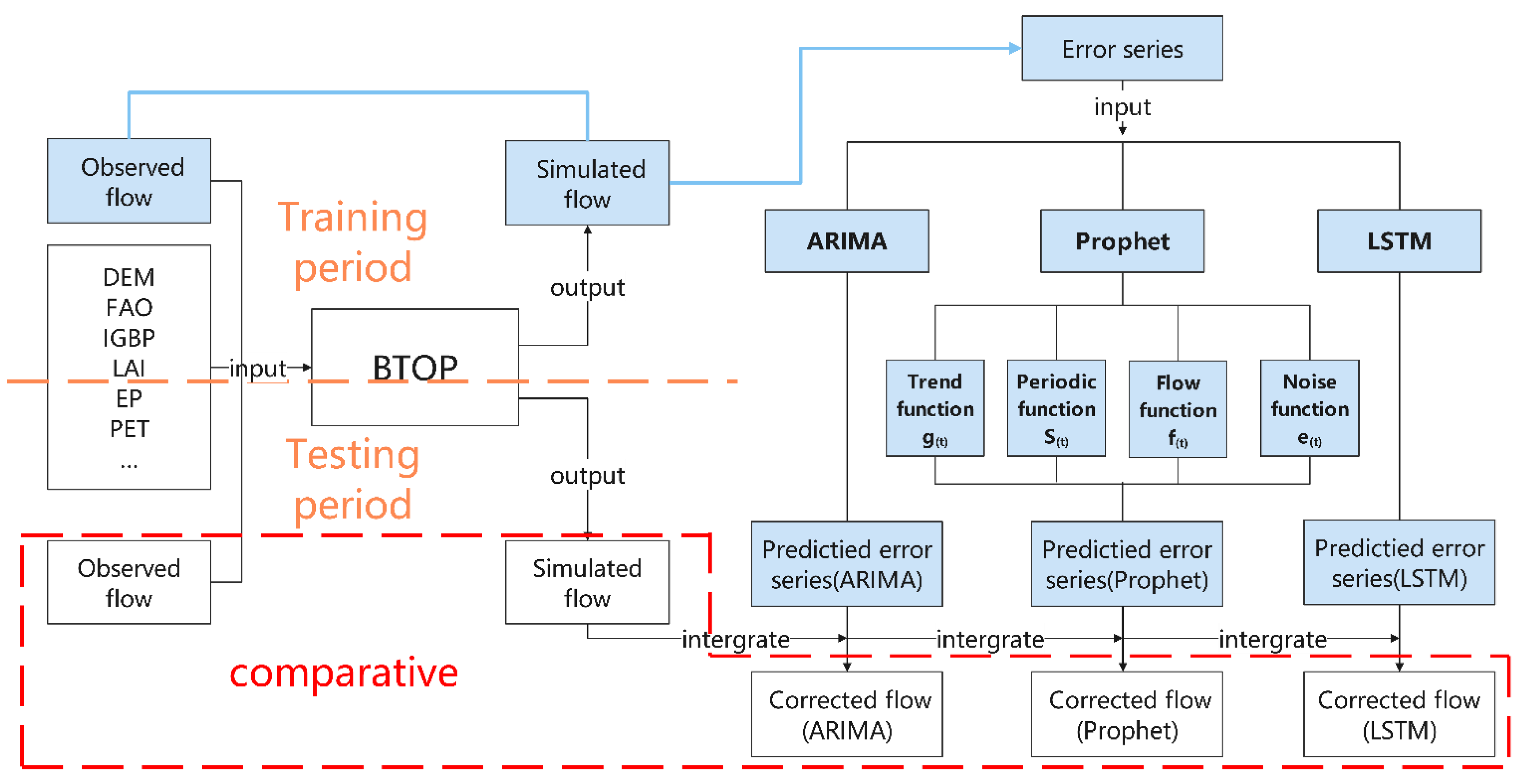
Firstly, the BTOP model simulates runoff in the training period. The parameters are automatically optimized and input into the BTOP model to simulate runoff during the testing period. Then, the simulated runoff flow is compared with the observed flow to obtain the error series of the training period, which is used as the input value of the time series model. After normalized pre-processing of the error series, the Prophet, LSTM, and ARIMA models are used to predict the time series of the training period error sequence, and the predicted error series of the testing period is obtained. Finally, the predicted error series is used to correct the simulated flow to obtain the corrected flow. Five indicators are used to compare the corrected flow and the original simulated flow: the NSE index, Pearson correlation coefficient R, mean absolute error (MAE), root mean square error (RMSE), and mean absolute percentage error (MAPE) (Figure 4).

4. Results and Discussion

The results are presented in two ways. On the one hand, a representative flow station was selected to specifically analyze the correction principles of the three time series models; this is presented in Section 4.1. The Donglin Station which had noticeable runoff pattern changes and good model modification results, was selected as an example to demonstrate the Prophet model and the other two comparison models in detail. On the other hand, an overall comparison of the correction effects of the three time series models at the four flow stations using evaluation metrics is presented in Section 4.2.

4.1. Performance of Each Time Series Model

4.1.1. Performance of ARIMA Model

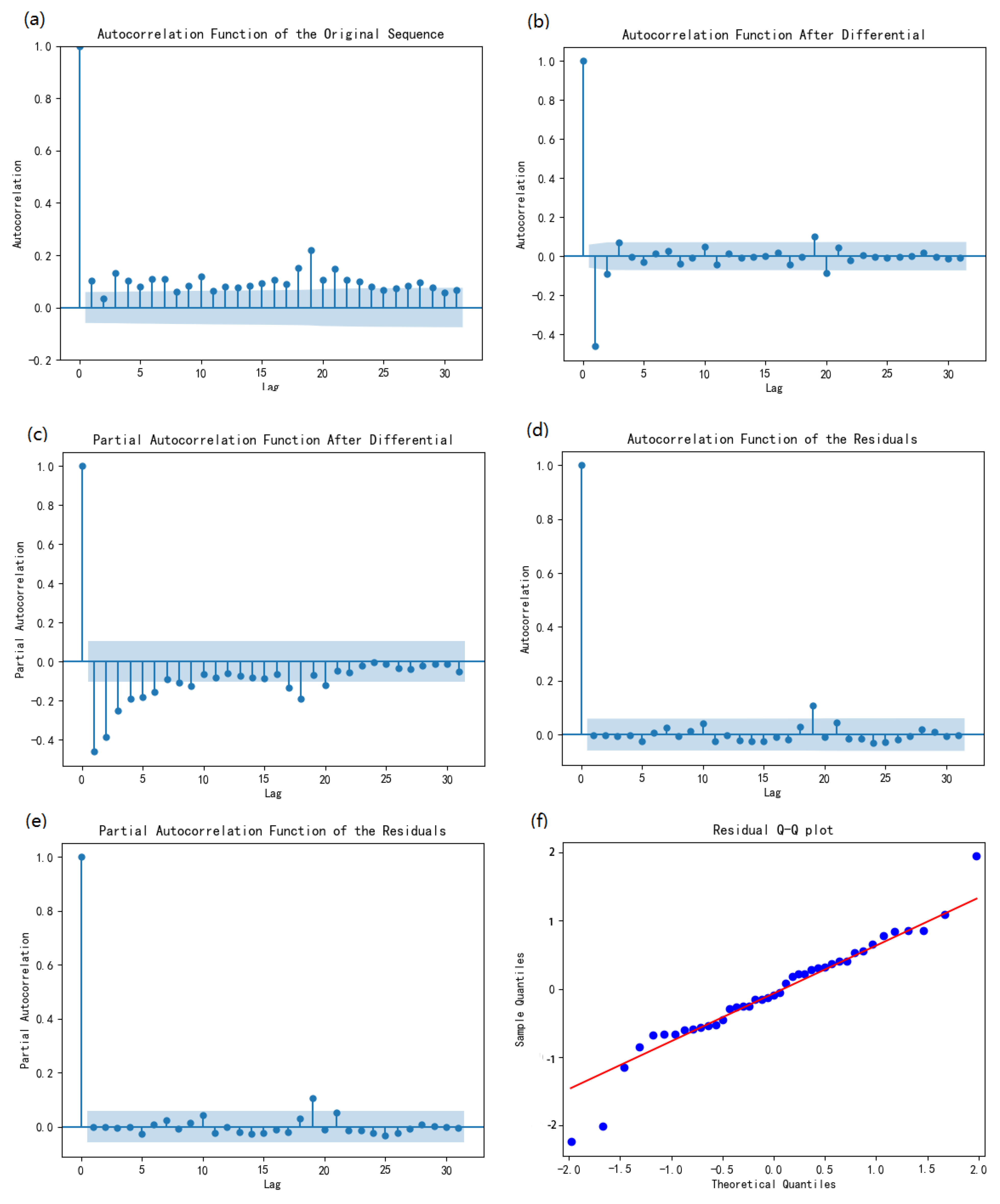
The error series of the Donglin station rate periodically was first tested by the augmented Dickey–Fuller (ADF) test (ADF less than 0.05 is considered as stationary series) [51,52] and plotted with autocorrelation, see Figure 5a in which it can be seen that the correlation coefficient of the original series is greater than zero for a long time, indicating a strong long-term correlation between the series. However, the p value corresponding to the ADF test statistic of the original sequence was 0.99, which was significantly greater than 0.05, indicating that the series is a non-stationary series (non-stationary series must not be a white noise series). Next, the original error series were made a first-order difference, followed by ADF detection and white noise detection. The results show that the autocorrelation plot has a solid short-term correlation, and the p values of both ADF and white noise test statistics are less than 0.05, so the error series after the first-order difference is a stationary non-white noise series.
By observing the ACF (autocorrelation function) and PACF (partial autocorrelation function) plots after differencing (Figure 5b,c), we can see that both ACF and PACF show smearing, the PACF cut-off is at lag 6, and ACF decay tends to zero after lag 1, so it is ARMA (6, 1) [53]. Finally, ARIMA (6, 1, 1) can be determined by combining first-order differences. Next, the error series of the testing period was simulated, the predicted results were fitted to the true values, and the residual series were analyzed (Figure 5d–f). The residual series in the figure is within the confidence interval above and below the mean 0, and the residual series passes the white noise test [54]. The result of the D-W test [55] on the residuals is 2.002, which is close to 2, indicates that there is no autocorrelation in the residuals predicted by the model, and the sample quantile distribution in the residual Q-Q plot is similar to the theoretical quantile distribution. All of this shows that the fitted model has good prediction.
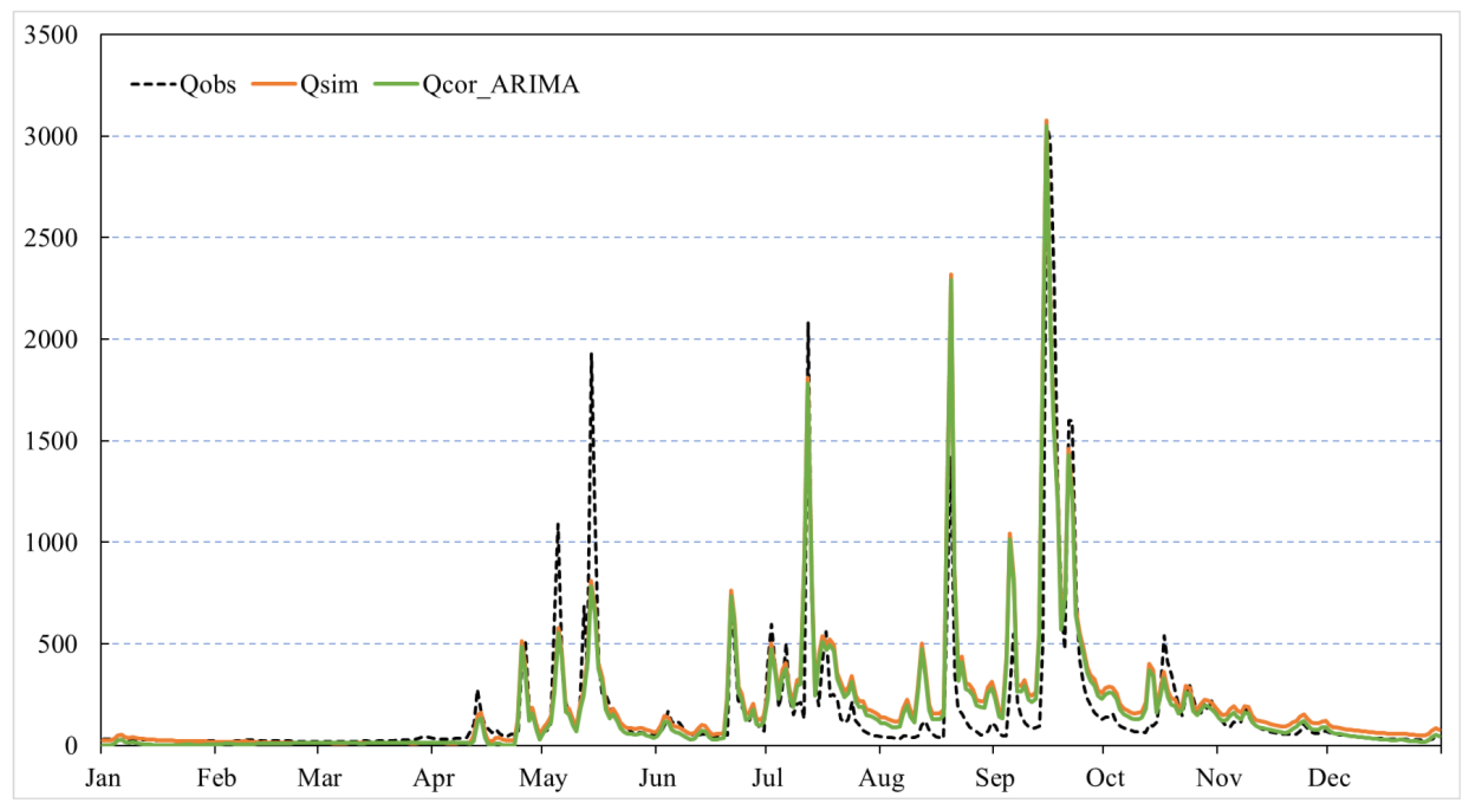
Figure 6 is the runoff simulation diagram obtained using the ARIMA model to correct the simulated runoff from the BTOP model. It can be seen that the modified curve of the ARIMA model effectively reduces a certain amount of runoff in the low flow periods to make it closer to the observed flow, which reduces the error to a certain extent and improves the simulation accuracy of the model. However, the modification of the ARIMA model in both the low-flow and high-flow periods is used to reduce runoff based on the original BTOP simulation trend. This is because the ARIMA model is, after all, only a model with statistical significance, the simulation of the hydrological process lacks physical cause analysis, and the simulation of the error series is only based on the information input before this period; thus, it may be difficult to deal with the turning point of the maximum value in the period of high flow. Therefore, measures should be taken in the practical application [56]. In general, the ARIMA model relies on the time-series dependence of forecast errors so that the errors will accumulate rapidly in the extrapolation process, and it is not suitable for larger basins or situations requiring longer forecasting periods [57].

4.1.2. Performance of LSTM Model

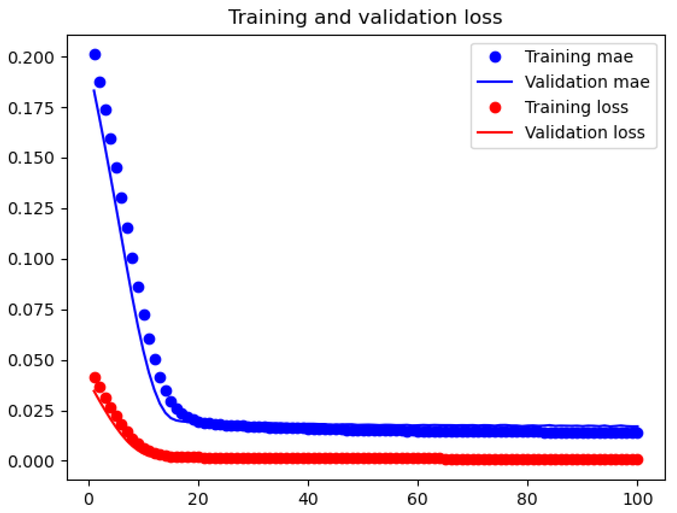
To improve the model accuracy, precipitation series were added for multivariate prediction in addition to the error series. The training dataset uses the simulated BTOP values from 1982 to 1984, and the 1985 data is the testing dataset. The input data are first normalized to make each feature variable contribute equally to the results, speed up the model iteration and improve the model accuracy. After many rounds of debugging, the model training parameters are: leaning_rate = 0.001, units = 20, batch_size = 5, epochs = 100. Due to the small amount of training data and the number of training sessions, overfitting occurs in the parameter debugging, so the regularization method is introduced. Figure 7 shows the loss of the training process. We can see that the MAE and loss decrease significantly in both the training and testing sets, and level off after 80 iterations, indicating that the LSTM model fits well.
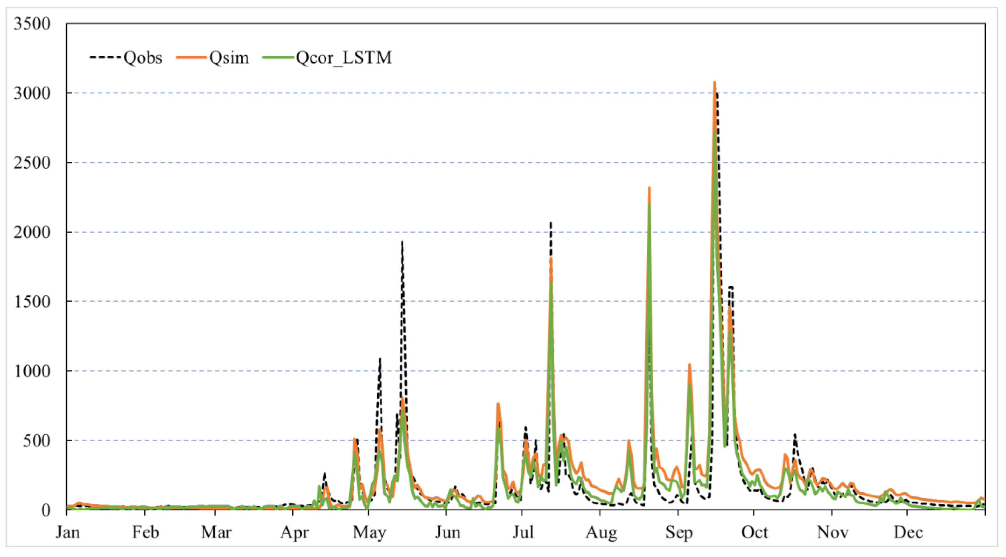
Figure 8 is the runoff simulation diagram obtained by using the LSTM model to correct the BTOP model. It can be seen that the corrected green curve trend of the LSTM is more consistent with the observed flow, and the error is reduced in most of the low-flow seasons. However, runoff has reduced slightly at the same maximum point rather than increased, mainly because the LSTM during practice is the trend of the error sequence in learning, without considering the error that comes from different scenarios. That is, there is no difference when handling the high-flow and low-flow season of the error sequence. As a result, the correction effect is not as good as the Prophet model [58,59]. In fact, different forecast scenarios and their corresponding forecast error distributions are important information for predicting the magnitude of forecast errors in future periods [60,61].

4.1.3. Performance of Improved Prophet Model

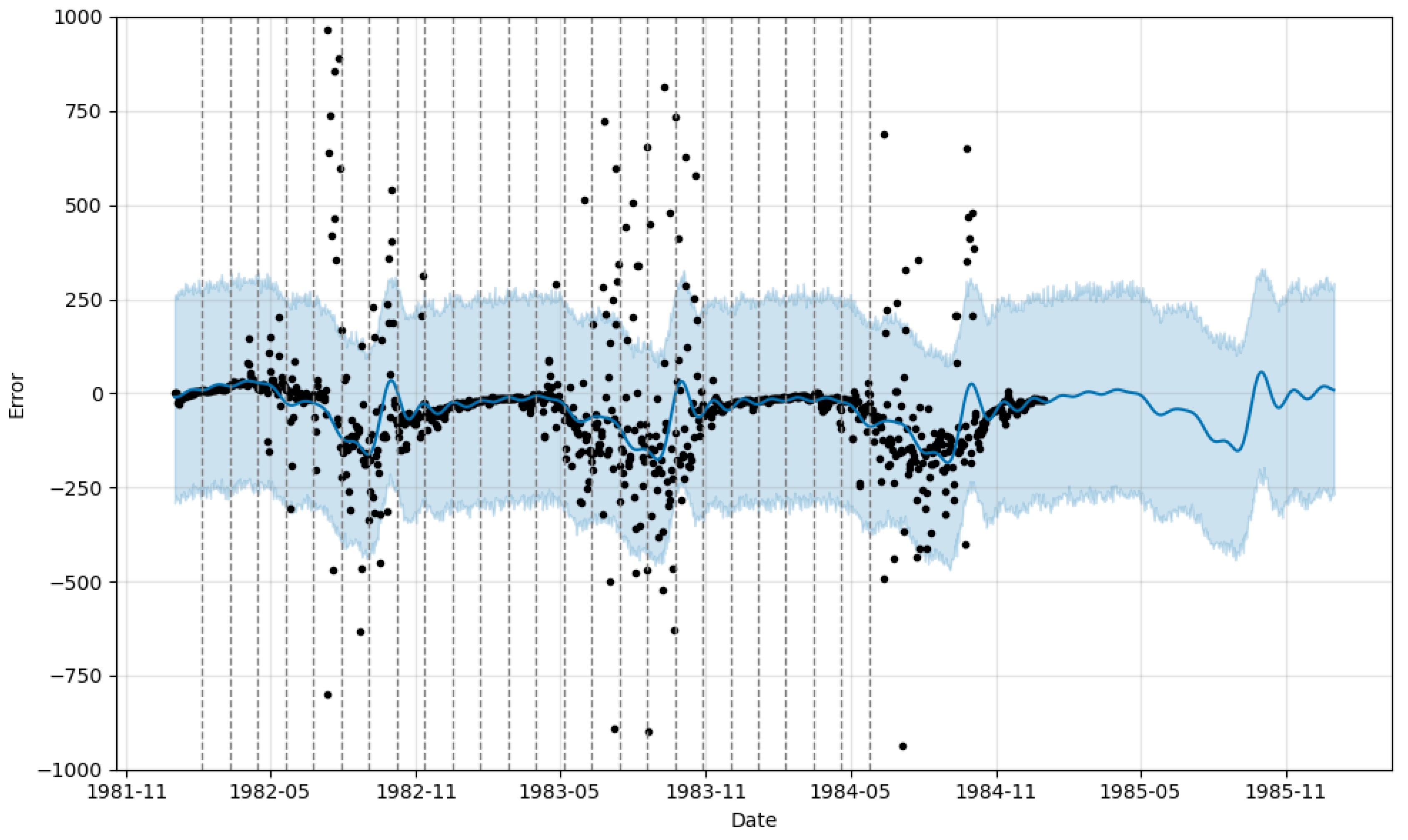
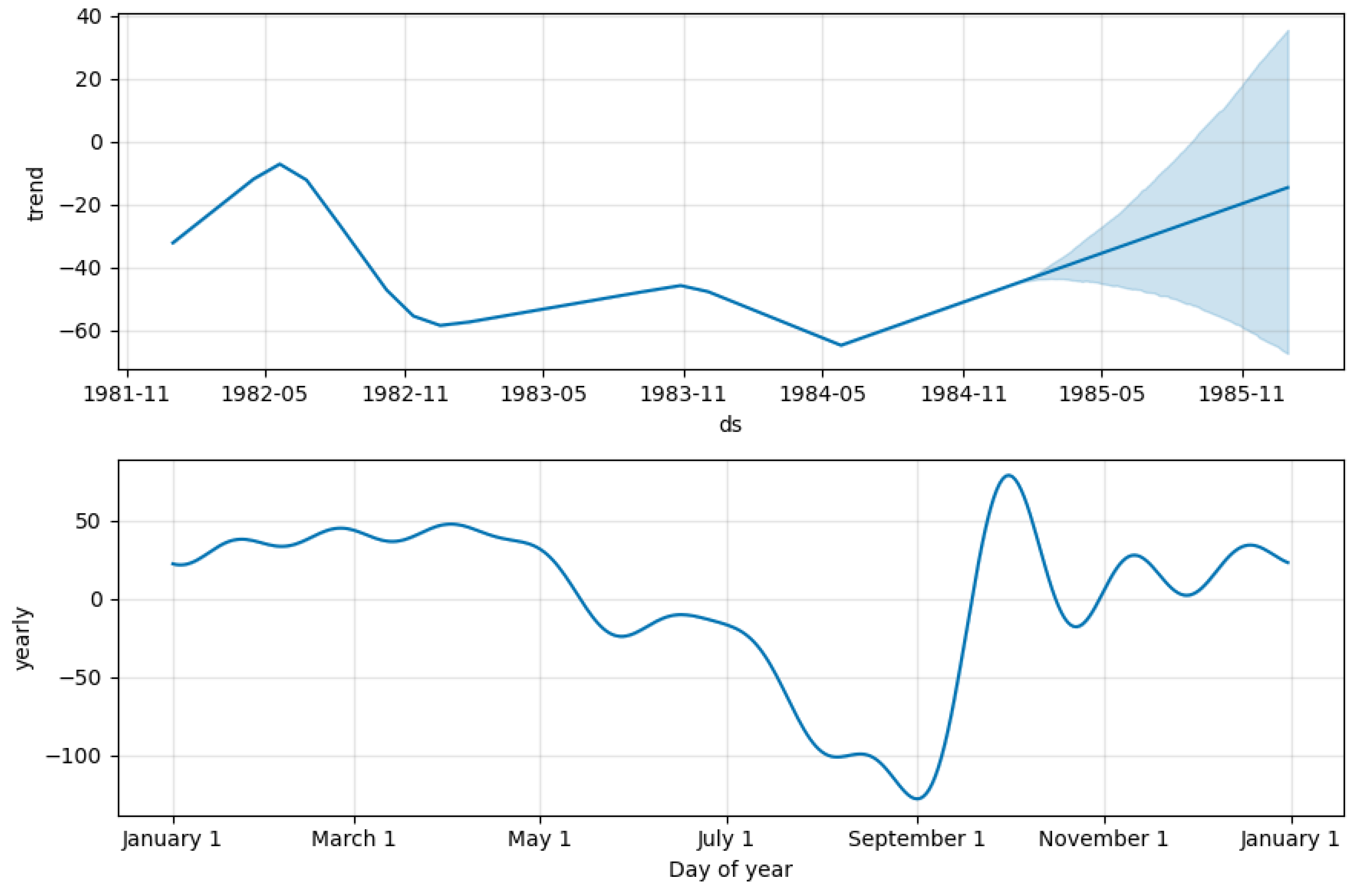
Several parameter rates were determined, and Figure 9 shows the analysis results of the error time series. This is an overall forecast result graph in which only the first 80% of the time series infer the point of change so that there is enough runway to predict the direction of the trend and avoid over-fitting the fluctuation at the end of the time series. In the evaluation of the results, the blue curve is used as the basis for prediction. The light blue confidence region is used for reference to improve the model. Looking at the trend analysis in Figure 10, it can be seen that the variation trend of the error series starts to decline in May, and then increases significantly from September to November, that is, the error in high-flow periods is bigger than in low-flow periods, which is closely related to the simulation of the BTOP model in-high flow and low-flow periods. The trend in the predicted value dramatically correlates with the change in the historical value and the current error situation [46].
Figure 11 is the runoff simulation diagram obtained using the Prophet model to correct the BTOP model. From the curves of the observed and simulated values therein, it can be seen from the observed and simulated curves that the BTOP model has achieved a good daily runoff simulation effect in the study area, the base simulated flow is close to the observed flow, and the flood peak simulation time is accurate [62]. Careful analysis of the error sources shows that the simulated flow of BTOP is generally slightly higher than the observed flow during the low-flow periods, while the simulated flood peak flow is much smaller than the observed flow in high-flow periods, which is the result of the transmission of BTOP model operation error from upstream to downstream [61]. Next, by looking at the Prophet correction curve, it can be found that the corrected runoff curve is closer to the observed flow in the low-flow periods. It also has a good correction effect in high-flow periods, but is not as significant as in low-flow periods. This indicates that the revision of the Prophet model is mainly reflected in reducing runoff through g t and s t in low-flow periods, and increasing runoff through f t in the maximum high-flow periods. However, for the few events where the simulated BTOP values are too large during the high-flow periods, the Prophet model only slightly reduces the runoff and is not effectively corrected (20 August). This is also the focus of further improvement of the model.
In general, the correction of runoff errors for BTOP using the Prophet model is effective.

4.2. Comprison between Three Time Series Models

This section analyzes the four hydrologic stations in the research area from the macroscopic perspective. Two types of indicators were used to evaluate the simulation effect of hydrological models and the correction effect of three time series models. The first is the hydrologic index NSE, R (the closer the NSE and R values are to 1, the better the simulation is, and an NSE greater than 0.7 indicates that the hydrological model simulated well). The other is the error index, that is, MAE, RMSE and MAPE (the error index of the time series model and the error index of the original BTOP model are converted to get the reduction rate, thus the larger the reduction rate, the better the model modification effect).
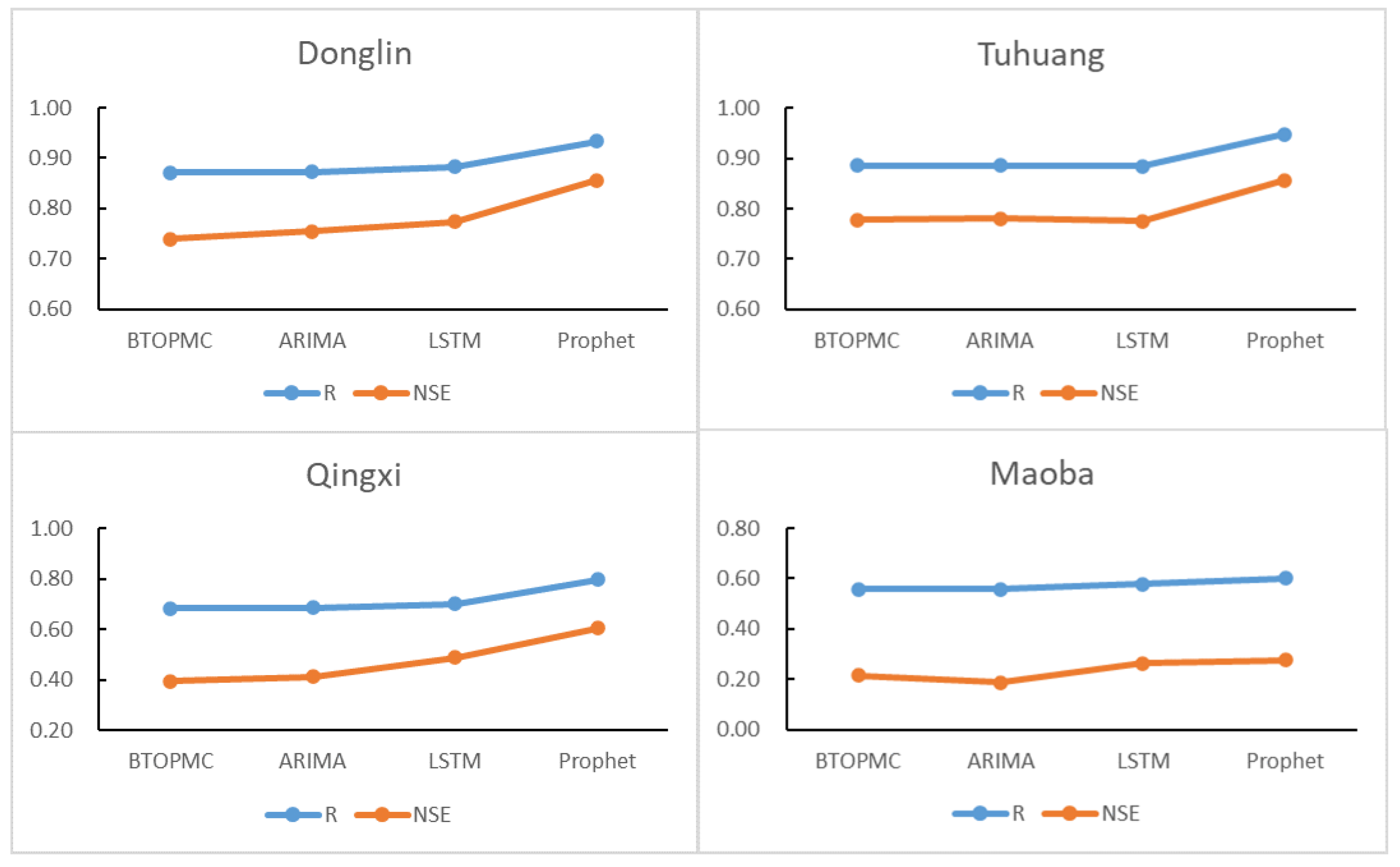
A comparison of the R and NSE of the three time series models and the original BTOP model is shown in Figure 12. We can see that the R and NSE of the runoff series were improved at all four stations, among which the Prophet model has the most significant improvement effect (NSE increased by an average of 30% and R increased by an average of 10%). Although the improvement effect of the LSTM and ARIMA models is not particularly obvious, mainly because they only predict the terminal error without considering the actual situation and runoff pattern characteristics, it also proves that it is effective to use the time series model to conduct runoff simulation correction for BTOP.
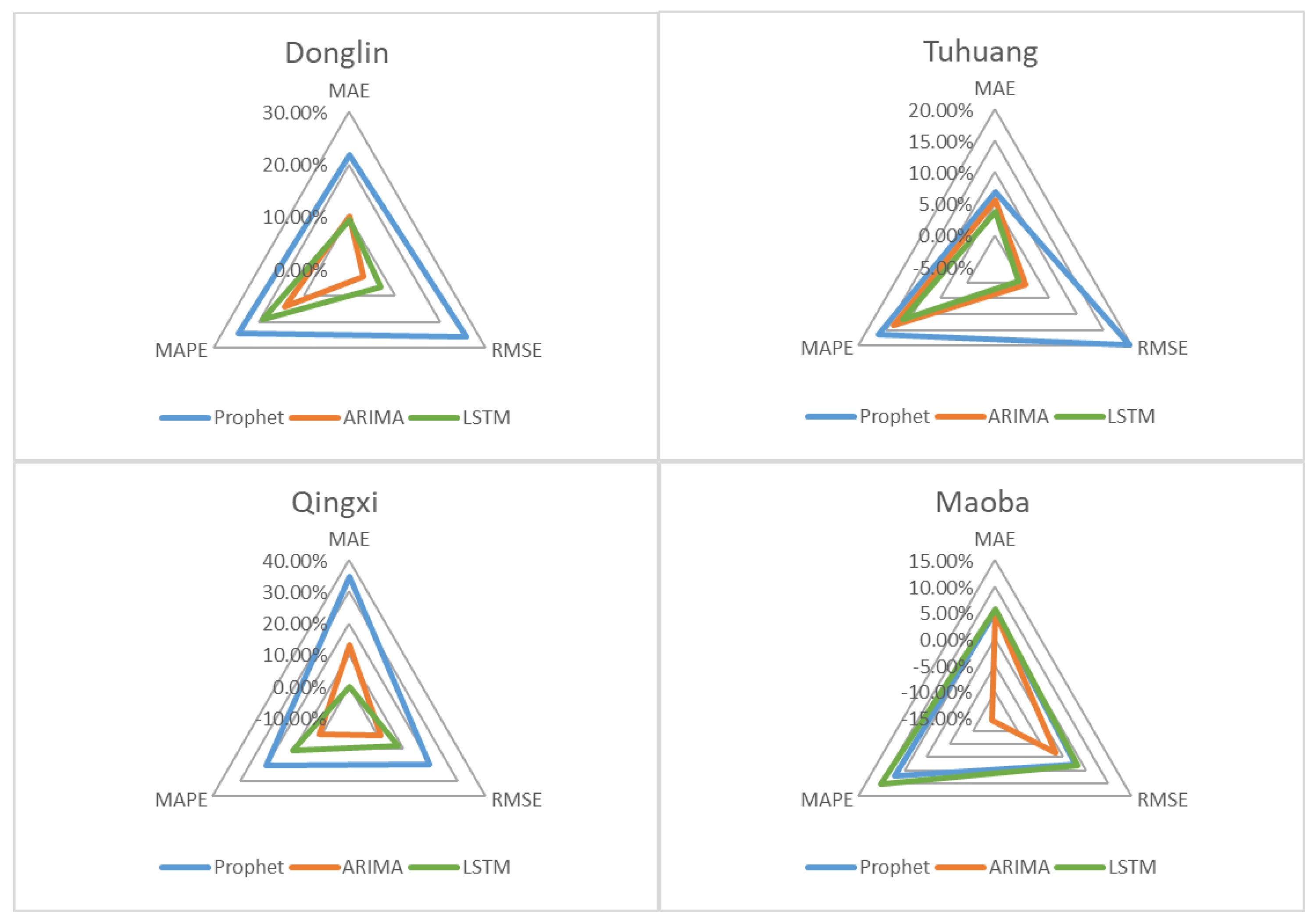
The error reduction rate of MAE, RMSE and MAPE were compared. As can be seen in Figure 13, the corrections of the three models basically show positive effects in all three error indexes compared to the original BTOP simulations. The larger the triangle is, the greater the error reduction rate is, the better the model modification effect is. Finally, the correction effects of the three time models are discussed separately for different hydrological model simulation effects.
(1)
At Donglin and Tuhuang stations, where BTOP simulations are better, MAE, RMSE and MAPE decreased by 6.94%~21.06%, 19.75%~25.74%, and 16.41%~24.49%, respectively, after Prophet modification. At this time, the Prophet model has a good correction effect, but the LSTM and ARIMA models have a poor effect, and the reduction rate of the corresponding error index after correction is far less than that of the Prophet model.
(2)
At Qinxi station, where the BTOP simulation is slightly less effective, MAE, RMSE, and MAPE decreased by 34.91%, 19.29% and 20.3%, respectively, after Prophet modification. At this time, the Prophet model is also well modified, and the effects of LSTM and ARIMA models are improved, but the reduction rate of the corresponding error index after modification is still less than half of that of the Prophet model.
(3)
At Maoba station, where the BTOP simulation is the least effective, MAE, RMSE and MAPE decreased by 5.15%, 2.61% and 7.05% after Prophet modification. At this time, the modified effect of the Prophet model began to decline, and the error reduction rate after the modification of LSTM and ARIMA models was close to that of the Prophet.
In general, the error reduction rate after correction of the Prophet model is the largest, and the reduction rate of each error indicator is about 1.7 times and 2.1 times that of the LSTM and ARIMA models, respectively. In addition, the better the simulation effect of the hydrological model is, the more the advantages of the Prophet model effect can be reflected. Therefore, combining the hydrological and error index, we can conclude that the Prophet model has the best correction effect on BTOP, followed by the LSTM model, and the ARIMA model has the worst correction effect.

5. Summary and Conclusions

This study used three time series models to correct the hydrological model BTOP runoff simulation in the Xuanhan Section of the Zhou River, China. The error between the simulated and observed flow of the BTOP was taken as a random variable, and the Prophet, ARIMA, LSTM models were used to predict the error series. Finally, the predicted error was used to correct the simulated flow to achieve the effect of correcting the runoff simulation accuracy of the BTOP hydrological model. The corrected results were elaborated from the perspective of the overall effect and the individual analysis of causes. The summary and conclusions are as follows:
(1)
The simulation of the BTOP model in the Zhou River basin is excellent. When the BTOP hydrological model is used for simulation in the study area, the law of error can be followed. We can see that the simulated flow of BTOP is generally slightly higher than the observed flow during the low-flow periods, while the simulated flood peak flow is smaller than the observed flow in high-flow periods.
(2)
The integration of the BTOP model and three time series models, Prophet, LSTM, and ARIMA, effectively improved the simulated runoff from the BTOP model. Among them, the prophet model performed best.
(3)
The LSTM model has a poor correction effect in high-flow periods due to its lack of scenario prediction. The ARIMA model does not consider seasonal factors and outlier processing and lacks physical analysis of the causes, leading to poor simulation results in both high-flow and low-flow periods.
(4)
In this study, the holiday function h t in the Prophet model is improved to the flow function f t , which makes the sequence more consistent with the runoff pattern and makes up for the poor effect of the comparison models in the high-flow periods. The improved model can better predict the hydrological time series and greatly improve the runoff simulation accuracy of the hydrological model.
It can be concluded that the improved Prophet model proposed in this study can effectively modify the runoff simulation of the BTOP hydrological model. However, some shortcomings of the study can be considered, as the lack of hydrological stations in the watershed, and the model training period can be extended appropriately. In the application of the time series model, it is a trend in model development for analysts to integrate their domain expertise. More effective correction of the high-flow periods of the hydrological model should be considered in the future, and attention should also be paid to the pre-processing of data and scenario prediction.

Author Contributions

Q.X.: Conceptualization, Software, Methodology, Formal analysis, Data Curation, Visualization, Writing—original draft. L.Z.: Conceptualization, Methodology, Formal analysis, Writing—review and editing. X.X.: Formal analysis, Visualization. L.L.: Methodology, Formal analysis. X.L. (Xing Liu): Data Curation, Visualization. X.L. (Xiaodong Li): Data Curation. T.A.: Funding acquisition, Supervision. All authors have read and agreed to the published version of the manuscript.

Funding

This research was funded by the Regional Innovation Cooperation Program (2020YFQ0013) and Key R&D Project (2021YFS028) from the Science& Technology Department of Sichuan Province, Key R&D Project (XZ202101ZY0007G) from the Science and Technology Department of Tibet.

Institutional Review Board Statement

Not applicable.

Informed Consent Statement

Not applicable.

Data Availability Statement

Not applicable.

Acknowledgments

We gratefully acknowledge the anonymous reviewers for their comments and suggestions that improved this manuscript.

Conflicts of Interest

The authors declare no conflict of interest.

References

  1. Bhatt, D.; Mall, R.K. Surface Water Resources, Climate Change and Simulation Modeling. Aquat. Procedia 2015, 4, 730–738. [Google Scholar] [CrossRef]
  2. Croley, T.E.; He, C. Distributed-Parameter Large Basin Runoff Model. I: Model Development. J. Hydrol. Eng. 2005, 10, 173–181. [Google Scholar] [CrossRef]
  3. Li, D.; Wrzesien, M.L.; Durand, M.; Adam, J.; Lettenmaier, D.P. How much runoff originates as snow in the western United States, and how will that change in the future? Geophys. Res. Lett. 2017, 44, 6163–6172. [Google Scholar] [CrossRef] [Green Version]
  4. Salvadore, E.; Bronders, J.; Batelaan, O. Hydrological modelling of urbanized catchments: A review and future directions. J. Hydrol. 2015, 529, 62–81. [Google Scholar] [CrossRef]
  5. Liu, C.; Shan, Y. Impact of an emergent model vegetation patch on flow adjustment and velocity. In Water Management; Thomas Telford Ltd.: London, UK, 2021; pp. 1–42. [Google Scholar]
  6. Liu, C.; Shan, Y.; Sun, W.; Yan, C.; Yang, K. An open channel with an emergent vegetation patch: Predicting the longitudinal profiles of velocities based on exponential decay. J. Hydrol. 2019, 582, 124429. [Google Scholar] [CrossRef]
  7. Zhou, L.; Zhang, X.; Liu, L.; Chen, T.; Liu, X.; Ren, Y.; Zhang, H.; Li, X.; Ao, T. An Approach to Evaluate Non-Point Source Pollution in An Ungauged Basin: A Case Study in Xiao'anxi River Basin, China; IWA Publishing: London, UK, 2020. [Google Scholar]
  8. Esling, P.; Agon, C. Time-Series Data Mining. ACM Comput. Surv. 2013, 45, 11–12. [Google Scholar] [CrossRef] [Green Version]
  9. Box, G.E.P.; Jenkins, G.M. Time Series Analysis Forecasting and Control; Holden-Day: San Francisco, CA, USA, 1970; Volume 3. [Google Scholar]
  10. Lngkvist, M.; Karlsson, L.; Loutfi, A. A review of unsupervised feature learning and deep learning for time-series modeling. Pattern Recogn. Lett. 2014, 42, 11–24. [Google Scholar] [CrossRef] [Green Version]
  11. Arıkan, S.M. Recent advances in SAR interferometry time series analysis for measuring crustal deformation. Tectonophysics 2012, 514–517, 1–13. [Google Scholar]
  12. Nourani, V.; Baghanam, A.H.; Adamowski, J.; Kisi, O. Applications of hybrid wavelet-Artificial Intelligence models in hydrology: A review. J. Hydrol. 2014, 514, 358–377. [Google Scholar] [CrossRef]
  13. Liu, Y.; Ji, Y.; Liu, D.; Fu, Q.; Li, M. A new method for runoff prediction error correction based on LS-SVM and a 4D copula joint distribution. J. Hydrol. 2021, 598, 126223. [Google Scholar] [CrossRef]
  14. Montanari, A.; Brath, A. A stochastic approach for assessing the uncertainty of rainfall-runoff simulations. Water Resour. Res. 2004, 40, 75–88. [Google Scholar] [CrossRef]
  15. Cheng, C.; Li, Y.; Liu, L. Study on real-time flood prediction in Xijiang River Basin based on ArMA-GARCH Model. In Proceedings of the Chinese Society of Dam Engineering 2021 Annual Conference, Guangzhou, China, 11–12 November 2021; p. 7. [Google Scholar]
  16. Zhang, H.; Guo, S. Bayesian probabilistic flood forecasting system. Sci. Technol. Eng. 2004, 4, 74–75. [Google Scholar] [CrossRef]
  17. Jiao, W.; Long, H. Prediction correction of distributed hydrological model based on autoregressive model. J. Water Resour. Water Eng. 2015, 6. [Google Scholar] [CrossRef]
  18. The Data Set Is Provided by Geospatial Data Cloud Site, Computer Network Information Center, Chinese Academy of Sciences. Available online: http://www.gscloud.cn (accessed on 25 March 2022).
  19. LP DAAC-MCD12Q1. Available online: https://lpdaac.usgs.gov/products/mcd12q1v006/ (accessed on 25 March 2022).
  20. FAO Digital Soil Map of the World (DSMW). Available online: http://www.fao.org/land-water/land/land-governance/land-resources-planning-toolbox/category/details/en/c/1026564/ (accessed on 25 March 2022).
  21. Martens, B.; Miralles, D.G.; Lievens, H.; van der Schalie, R.; de Jeu, R.A.M.; Fernández-Prieto, D.; Beck, H.E.; Dorigo, W.A.; Verhoest, N.E. GLEAM v3: Satellite-based land evaporation and root-zone soil moisture. Geosci. Model Dev. 2017, 10, 1903–1925. [Google Scholar] [CrossRef] [Green Version]
  22. The Potential Evapotranspiration (EP) from the Climatic Research Unit (CRU) of the School of Environmental Sciences (ENV) at the University of East Anglia (UEA). Available online: http://www.cru.uea.ac.uk/ (accessed on 25 March 2022).
  23. The Leaf Area Index (LAI) of the National Centers for Environmental Information. Available online: https://www.ncei.noaa.gov/data/avhrr-land-leaf-area-index-and-fapar/access/ (accessed on 25 March 2022).
  24. Zhu, Y.; Liu, L.; Qin, F.; Zhou, L.; Zhang, X.; Chen, T.; Li, X.; Ao, T. Application of the Regression-Augmented Regionalization Approach for BTOP Model in Ungauged Basins. Water 2021, 13, 2294. [Google Scholar] [CrossRef]
  25. Gusyev, M.A.; Magome, J.; Kiem, A.; Takeuchi, K. The BTOP Model with Supplementary Tools User Manual; Public Works Research Institute (PWRI): Tsukuba, Japan, 2017. [Google Scholar]
  26. Takeuchi, K.; Ao, T.; Ishidaira, H. Introduction of block-wise use of TOPMODEL and Muskingum-Cunge method for the hydroenvironmental simulation of a large ungauged basin. Int. Assoc. Sci. Hydrol. Bull. 1999, 44, 633–646. [Google Scholar] [CrossRef]
  27. Tianqi, A.; Takeuchi, K.; Ishidaira, H.; Yoshitani, J.; Fukami, K. Development and application of a new algorithm for automated pit removal for grid DEMs. Int. Assoc. Sci. Hydrol. Bull. 2003, 48, 985–997. [Google Scholar] [CrossRef]
  28. Takeuchi, K.; Hapuarachchi, P.; Zhou, M.; Ishidaira, H.; Magome, J. A BTOP model to extend TOPMODEL for distributed hydrological simulation of large basins. Hydrol. Process. 2010, 22, 3236–3251. [Google Scholar] [CrossRef]
  29. Liu, L.; Zhou, L.; Li, X.; Ting; Ao, T. Screening and Optimizing the Sensitive Parameters of BTOPMC Model Based on UQ-PyL Software: Case Study of a Flood Event in the Fuji River Basin, Japan. J. Hydrol. Eng. 2020, 25, 5020030. [Google Scholar] [CrossRef]
  30. Zhou, L.; Rasmy, M.; Takeuchi, K.; Koike, T.; Selvarajah, H.; Ao, T. Adequacy of Near Real-Time Satellite Precipitation Products in Driving Flood Discharge Simulation in the Fuji River Basin, Japan. Appl. Sci. 2021, 11, 1087. [Google Scholar] [CrossRef]
  31. Zhou, L.; Koike, T.; Takeuchi, K.; Rasmy, M.; Onuma, K.; Ito, H.; Selvarajah, H.; Liu, L.; Li, X.; Ao, T. A study on availability of ground observations and its impacts on bias correction of satellite precipitation products and hydrologic simulation efficiency. J. Hydrol. 2022, 610, 127595. [Google Scholar] [CrossRef]
  32. Hapuarachchi, H.A.P.; Takeuchi, K.; Zhou, M.; Kiem, A.S.; Georgievski, M.; Magome, J.; Ishidaira, H. Investigation of the Mekong River basin hydrology for 1980–2000 using the YHyM. Hydrol. Process. 2008, 22, 1246–1256. [Google Scholar] [CrossRef]
  33. Takeuchi, K. Studies on the Mekong River Basin-Modelling of Hydrology and Water Resources. Hydrol. Process. 2008, 22, 1243–1245. [Google Scholar] [CrossRef]
  34. Liu, L.; Ao, T.; Zhou, L.; Takeuchi, K.; Gusyev, M.; Zhang, X.; Wang, W.; Ren, Y. Comprehensive evaluation of parameter importance and optimization based on the integrated sensitivity analysis system: A case study of the BTOP model in the upper Min River Basin, China. J. Hydrol. 2022, 610, 127819. [Google Scholar] [CrossRef]
  35. Shrestha, S.; Bastola, S.; Babel, M.S.; Dulal, K.N.; Magome, J.; Hapuarachchi, H.; Kazama, F.; Ishidaira, H.; Takeuchi, K. The assessment of spatial and temporal transferability of a physically based distributed hydrological model parameters in different physiographic regions of Nepal. J. Hydrol. 2007, 347, 153–172. [Google Scholar] [CrossRef]
  36. Ao, T.; Ishidaira, H.; Takeuchi, K.; Kiem, A.S.; Yoshitari, J.; Fukami, K.; Magome, J. Relating BTOPMC model parameters to physical features of MOPEX basins. J. Hydrol. 2006, 320, 84–102. [Google Scholar] [CrossRef]
  37. Duan, Q.Y.; Gupta, V.K.; Sorooshian, S. Shuffled complex evolution approach for effective and efficient global minimization. J. Optimiz. Theory App. 1993, 76, 501–521. [Google Scholar] [CrossRef]
  38. Bandura, E.; Jadoski, G.S.; Junior, G. Applications of the ARIMA model for time series data analysis. Appl. Res. Agrotechnol. 2019, 12, 145–150. [Google Scholar]
  39. Kavasseri, R.G.; Seetharaman, K. Day-ahead wind speed forecasting using f-ARIMA models. Renew. Energ. 2009, 34, 1388–1393. [Google Scholar] [CrossRef]
  40. Cong, M.; Li, Y. Improving Forecasting Accuracy of Annual Runoff Time Series Using RBFN Based on EEMD Decomposition. DEStech Trans. Eng. Technol. Res. 2017. [Google Scholar] [CrossRef] [Green Version]
  41. Rizkya, I.; Syahputri, K.; Sari, R.M.; Siregar, I.; Utaminingrum, J. Autoregressive Integrated Moving Average (ARIMA) Model of Forecast Demand in Distribution Centre. IOP Conf. Ser. Mater. Sci. Eng. 2019, 598, 12071. [Google Scholar] [CrossRef]
  42. Hochreiter, S.; Schmidhuber, J. Long short-term memory. Neural Comput. 1997, 9, 1735–1780. [Google Scholar] [CrossRef] [PubMed]
  43. Yu, Y.; Si, X.; Hu, C.; Zhang, J. A Review of Recurrent Neural Networks: LSTM Cells and Network Architectures. Neural Comput. 2019, 31, 1235–1270. [Google Scholar] [CrossRef] [PubMed]
  44. Alom, M.Z.; Taha, T.M.; Yakopcic, C.; Westberg, S.; Sidike, P.; Nasrin, M.S.; Hasan, M.; Essen, B.V.; Awwal, A.; Asari, V.K. A State-of-the-Art Survey on Deep Learning Theory and Architectures. Electronics 2019, 8, 292. [Google Scholar] [CrossRef] [Green Version]
  45. Duarte, D.; Walshaw, C.; Ramesh, N. A Comparison of Time-Series Predictions for Healthcare Emergency Department Indicators and the Impact of COVID-19. Appl. Sci. 2021, 11, 3561. [Google Scholar] [CrossRef]
  46. Taylor, S.J.; Letham, B. Forecasting at Scale. Am. Stat. 2017, 5, e3190v2. [Google Scholar] [CrossRef]
  47. Aditya Satrio, C.B.; Darmawan, W.; Nadia, B.U.; Hanafiah, N. Time series analysis and forecasting of coronavirus disease in Indonesia using ARIMA model and PROPHET. Procedia Comput. Sci. 2021, 179, 524–532. [Google Scholar] [CrossRef]
  48. Medina, I.; Montaner, D.; Tárraga, J.; Dopazo, J. Prophet, a web-based tool for class prediction using microarray data. Bioinformatics 2007, 23, 390–391. [Google Scholar] [CrossRef] [Green Version]
  49. Boykov, Y.; Kolmogorov, V. An experimental comparison of min-cut/max- flow algorithms for energy minimization in vision. IEEE Trans. Pattern Anal. 2004, 26, 1124–1137. [Google Scholar] [CrossRef] [Green Version]
  50. Devaraj, J.; Elavarasan, R.M.; Pugazhendhi, R.; Shafiullah, G.M.; Hossain, E. Forecasting of COVID-19 cases using Deep learning models: Is it reliable and practically significant? Results Phys. 2021, 21, 103817. [Google Scholar] [CrossRef]
  51. Tashman, L.J.; Leach, M.L. Automatic forecasting software: A survey and evaluation. Int. J. Forecast. 1991, 7, 209–230. [Google Scholar] [CrossRef] [Green Version]
  52. Elliott, G.; Rothenberg, T.J.; Stock, J.H. Efficient Tests for an Autoregressive Unit Root. Econometrica 1996, 64, 813–836. [Google Scholar] [CrossRef] [Green Version]
  53. Gep, B.; Gm, J. Times Series Analysis—Forecasting and Control; Prentice-Hall: Englewood Cliffs, NJ, USA, 1976. [Google Scholar]
  54. Mitic, P. Is a Reputation Time Series White Noise? In Proceedings of the International Conference on Intelligent Data Engineering and Automated Learning, Guilin, China, 30 October–1 November 2017. [Google Scholar]
  55. Hill, R.J.; Flack, H.D. The use of the Durbin–Watsondstatistic in Rietveld analysis. J. Appl. Crystallogr. 1987, 20, 356–361. [Google Scholar] [CrossRef]
  56. Shukur, O.B.; Lee, M.H. Daily wind speed forecasting through hybrid KF-ANN model based on ARIMA. Renew. Energ. 2015, 76, 637–647. [Google Scholar] [CrossRef]
  57. Kumar, S.V.; Vanajakshi, L. Short-term traffic flow prediction using seasonal ARIMA model with limited input data. Eur. Transp. Res. Rev. 2015, 7, 21. [Google Scholar] [CrossRef] [Green Version]
  58. Xu, D.; Zhang, Q.; Ding, Y.; Zhang, D. Application of a hybrid ARIMA-LSTM model based on the SPEI for drought forecasting. Environ. Sci. Pollut. R. 2021, 29, 4128–4144. [Google Scholar] [CrossRef]
  59. Vlachas, P.R.; Byeon, W.; Wan, Z.Y.; Sapsis, T.P.; Koumoutsakos, P. Data-Driven Forecasting of High-Dimensional Chaotic Systems with Long Short-Term Memory Networks. Proc. R. Soc. A Math. Phys. Eng. Sci. 2018, 474, 20170844. [Google Scholar] [CrossRef] [Green Version]
  60. Sherstinsky, A. Fundamentals of Recurrent Neural Network (RNN) and Long Short-Term Memory (LSTM) Network. Phys. D: Nonlinear Phenom. 2020, 404, 132306. [Google Scholar] [CrossRef] [Green Version]
  61. Greff, K.; Srivastava, R.K.; Koutník, J.; Steunebrink, B.R.; Schmidhuber, J. LSTM: A Search Space Odyssey. IEEE Trans. Neural Netw. Learn. Syst. 2016, 28, 2222–2232. [Google Scholar] [CrossRef] [Green Version]
  62. Gusyev, M.A.; Kwak, Y.; Khairul, M.I.; Arifuzzaman, M.B.; Magome, J.; Sawano, H.; Takeuchi, K. Effectiveness of water infrastructure for river flood management: Part 1—Flood Hazard Assessment using hydrological models in Bangladesh. Proc. Int. Assoc. Hydrol. Sci. 2015, 370, 75–81. [Google Scholar] [CrossRef] [Green Version]
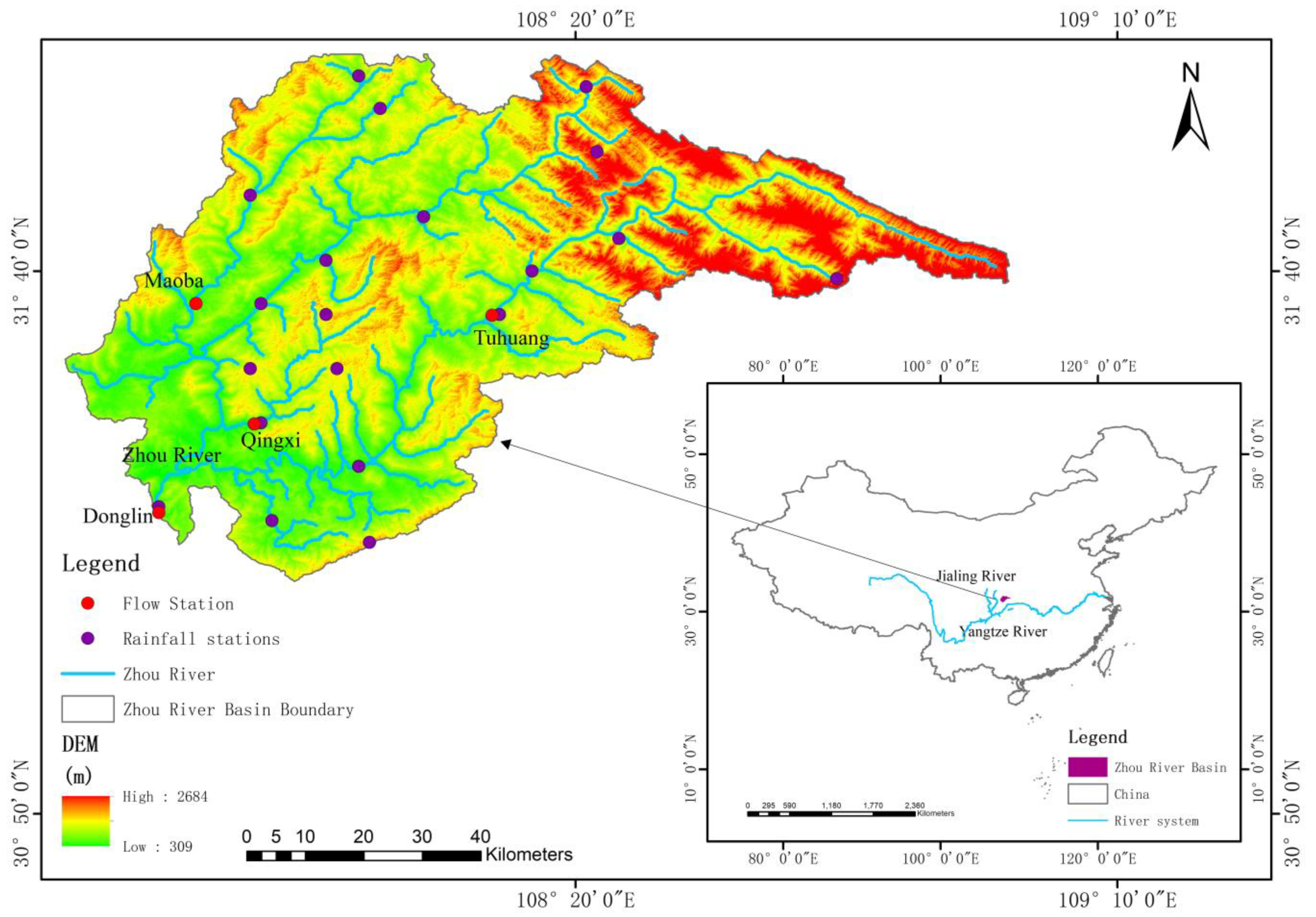
Figure 1. Location, digital elevation model (DEM), and ground observations in the Zhou River Basin (the Zhou River is a first-class tributary of the Jialing River).
Applsci 12 06883 g001
Figure 2. LSTM working principle. The three σ are the forget gate, the input gate and the output gate. is the dot product operation. C t denotes the cell state, X t denotes the input data and h t denotes the output data.
Applsci 12 06883 g002
Figure 3. The principle of the Prophet model for prediction.
Applsci 12 06883 g003
Figure 4. The framework of this study.
Applsci 12 06883 g004
Figure 5. Prediction process of ARIMA model. (a) Original sequence autocorrelation, (b) autocorrelation and (c) partial autocorrelation after difference, (d) residual autocorrelation and (e) partial autocorrelation, (f) residual Q-Q graph.
Applsci 12 06883 g005
Figure 6. Hydrographs from Donglin Station in 1985 with observed, simulated, and ARIMA correction runoff.
Applsci 12 06883 g006
Figure 7. Loss function process of LSTM model.
Applsci 12 06883 g007
Figure 8. Hydrographs from Donglin Station in 1985 with observed, simulated, and LSTM correction runoff.
Applsci 12 06883 g008
Figure 9. Error forecast of the Prophet model. The black dots represent the historical input data, the blue line represents the predicted trend line after model fitting, the light blue area above and below the blue curve represents the confidence interval, and the gray dotted-line reflects the position of the trend mutation point of the sequence.
Applsci 12 06883 g009
Figure 10. Trend prediction analysis of Prophet model. The blue line shows the trend that the model fits from the test data, and the light blue shade shows the predicted trend.
Applsci 12 06883 g010
Figure 11. Hydrographs from Donglin Station in 1985 with observed, simulated, and Prophet correction runoff.
Applsci 12 06883 g011
Figure 12. Comparison of R and NSE for four sites under different model corrections.
Applsci 12 06883 g012
Figure 13. Comparison of error reduction rate for four sites under different model corrections.
Applsci 12 06883 g013
Table 1. Example of Prophet model parameter setting.
Parameter NatureParameter NameValue
Trend parametersgrowthlinear
changepointsNone
n_changepoints25
changepoint_range0.8
changepoint_prior_scale0.5
Periodic parametersyearly_seasonality10
weekly_seasonalityfalse
daily_seasonalityfalse
seasonality_modeadditive
seasonality_prior_scale20
Flow parametersflowflow
flow_prior_scale10
Other parametersmcmc_samples0
interval_width0.8
uncertainty_samples1000
stan_backendcmdstanpy
Publisher’s Note: MDPI stays neutral with regard to jurisdictional claims in published maps and institutional affiliations.