Article

Genetic Algorithm-Based Intelligent Selection Method of Universal Shield Segment Assembly Points

1
School of Mechanical Science and Engineering, Huazhong University of Science and Technology, Wuhan 430074, China
2
State Key Lab of Digital Manufacturing Equipment & Technology, Huazhong University of Science and Technology, Wuhan 430074, China
*
Author to whom correspondence should be addressed.
Appl. Sci. 2022, 12(14), 6926; https://doi.org/10.3390/app12146926
Submission received: 11 June 2022 / Revised: 5 July 2022 / Accepted: 6 July 2022 / Published: 8 July 2022
(This article belongs to the Topic Pipeline and Underground Space Technology)

Abstract

:
The proportion of universal segment in tunnel construction is constantly increasing. A key factor affecting the quality of tunnel construction is the selection of the shield segment assembly points. Nevertheless, the quality and efficiency of the current manual selection method cannot be guaranteed. To realize a high correct rate, high efficiency and intelligence of universal segment assembly points selection, an intelligent selection method of assembly points is proposed. First, the objective function is established by considering the thrust cylinder stroke and shield tail gap differences. Second, to adaptively optimize the weights of the objective function, the working conditions are divided into 81 intervals, and a genetic algorithm is proposed to optimize weights in each interval. Third, a Monte-Carlo-based method is proposed to generate an example dataset, which is used for the genetic algorithm to optimize the weights. Finally, the proposed method was applied to the segment assembly points selection for Line 8 of the Zhengzhou rail transit in China. The results show that the method of assembly segment selection can reach a 90.6% correct rate in the field. The research results of this paper can be used for the selection of the universal shield segment assembly points.

1. Introduction

Shield construction is an advanced tunnel construction method in soft soil, which is widely used in subway tunnels [1,2], water conservancy tunnels [3,4] and highway tunnels [5]. During construction, the shield machine pushes forward on the assembled segments and assembles new segment rings under the support of the tail shield, and the assembled segment rings form the final tunnel [6,7,8,9,10]. As a kind of advanced tunnel lining, the universal segment ring is a kind of ring with a certain amount of wedge. Only one type of universal segment ring is needed for the whole construction process to complete the tunnel assembly. Only one set of molds is needed, and its proportion in the construction is increasing [11,12,13]. To improve the quality of formed tunnels, some scholars have studied the load on the segment ring [14,15], while others have focused on the selection of the segment assembly point. The selection of the segment assembly point is the first step in segment assembly and is a critical step in tunnel construction. However, at present, the construction of the universal segment of the assembly point is mainly determined by the shield machine drivers with experience, which not only limits the construction speed and increases the work intensity of drivers, but also the quality of the selected assembly point is not guaranteed due to the subjective factors of drivers [16,17]. The unreasonable selection of a segment assembly point often leads to serious engineering accidents, such as uncontrolled attitude of the shield machine, broken segments and the inability to fit the design tunnel axis (DTA) [18]. Therefore, the intelligent and reasonable selection of universal shield segment assembly points is an urgent problem to be solved.
Basically, two approaches are used to select the segment assembly points in the current study. The first approach is to select the assembly points with the aim of reducing the deviation between the actual axis and the DTA. Some research has been conducted in this regard. In the papers [16,17,19], the authors derived the calculation method of the center of the front face of the segment ring after assembling the segment with different assembly points used the exhaustive method to calculate the curve-fitting deviation corresponding to all assembly points and then selected the point with the smallest deviation as the best assembly point. However, in practice, various construction factors have a huge impact on the selection of the assembly point of the segment, and a selection method that only reduces the deviation of the axis fitting has little applicability in actual construction. Therefore, more studies focus on the second approach of the selection of an assembly point, which is to select the assembly point with the goal of adjusting construction factors. Hu et al. [20] derived a calculation method for the amount of change in the shield tail gap for selecting different assembly points, which provides a reference for assembly point selection considering the shield tail gap, but this study does not explain how to choose the assembly points. Liu [21] determined the objective function for optimizing the shield tail gap difference and curve-fitting deviation, but how the weights of each parameter are taken is not described. Zhang et al. [22] established the objective function of segment assembly point selection considering the shield tail gap, thrust cylinder stroke difference and lining trend, and the weights of each parameter were determined manually in real time, but this weight-taking method is easily influenced by human subjective actions, and the process is tedious. Miao [23] established an objective function with shield tail gap, thrust cylinder stroke difference and curve-fitting deviation as the influencing parameters, but the weights are still given empirically. Zhao et al. [24] analyzed the influencing factors of segment assembly point selection and designed an objective function; one step further is that the weights of the objective function can be adaptively changed, but the method of taking the weights has no theoretical support.
It can be noted that establishing the objective function of the selection of a segment assembly point has become the major research method for selecting the assembly point. There are two key steps in the establishment of a reasonable objective function. One is the selection of the influencing factors, and the other is taking the weights of the influencing factors. It is clear that the most important influencing factors are thrust cylinder stroke difference and shield tail gap. The proportion of the curve-fitting deviation in the objective function is small. For example, in the paper [24], the authors take an initial weight of 5%. In addition, the curve-fitting deviation cannot be accurately calculated due to the drift phenomenon of the newly assembled segment. Meanwhile, engineering has agreed that considering the thrust cylinder stroke difference and the shield tail gap are sufficient parameters to select the assembly point. On the other hand, the weights of the influencing factors have a crucial influence on the rationality of the selection of assembly points. However, in the current study, the weight of each parameter is determined by the drivers through experience. This weighting method is arbitrary and subjective, making it impossible to guarantee the reasonableness of weights and resulting in the research results not reaching the ideal application in engineering. At the same time, the weights reflect the importance degree of the parameters at that moment, and the importance degree of each parameter changes constantly under different working conditions. Therefore, the weights should also be adjusted with the working conditions all the time. However, how to adjust the weights scientifically and reasonably is also a gap in the current research.
The purpose of this paper is to establish an objective function of the selection of the segment assembly point with thrust cylinder stroke difference and shield tail gap and use a scientific method to objectively and adaptively take the weights. The thrust cylinder stroke difference and shield tail gap represent the working condition, so they are collectively referred to as working condition parameters (WCPs) in this paper. Essentially, the problem of segment assembly point selection is a multi-objective optimization problem. The solution of multi-objective optimization problems is mostly calculated by intelligent optimization algorithms, such as ant colony algorithm [25,26], particle swarm optimization [27,28], a genetic algorithm [29,30,31,32], etc. Among them, the genetic algorithm has been widely used in solving multi-objective optimization problems because of its good robustness and strong global search ability, and we will use genetic algorithms to optimize the weights in this paper. To achieve adaptive taking of weights with WCPs, we divide the working conditions into 81 intervals. The working conditions are considered to be consistent within each interval and share the same set of weights, and the genetic algorithm optimizes the weights within each interval. We use the correct rate of assembly point selection for example data as an evaluation index of the chromosome goodness of the genetic algorithm. However, actual data from the project are not only slow to obtain, but also difficult to reasonably reflect all working conditions. So, we also propose a method to calculate WCPs and combine them with a manual labeling method to obtain a sufficient number of example data. Figure 1 shows the pipeline of the work in this paper.
The remainder of this paper is organized as follows. Section 2 establishes the assembly point selection objective function. Section 3 presents the calculation method of the WCPs and the establishment of an example dataset. In Section 4, we demonstrate the architecture of the genetic algorithm; Section 5 shows the optimization results of weights by genetic algorithm and the test results of the proposed method. Finally, Section 6 gives the conclusions.

2. Establishment of Assembly Point Selection Objective Function

2.1. Related Concepts

2.1.1. Overview of Segment Assembly

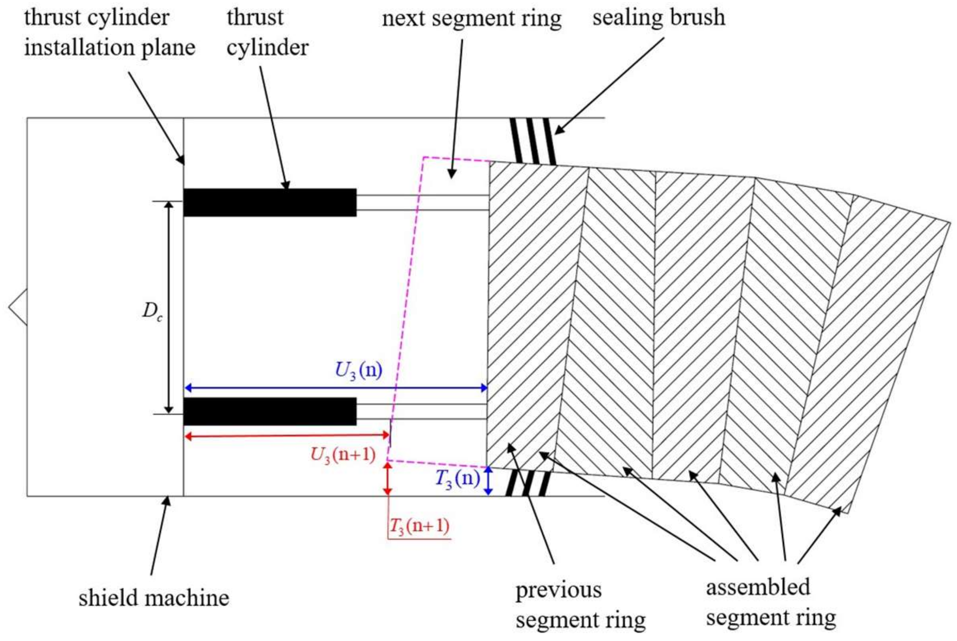
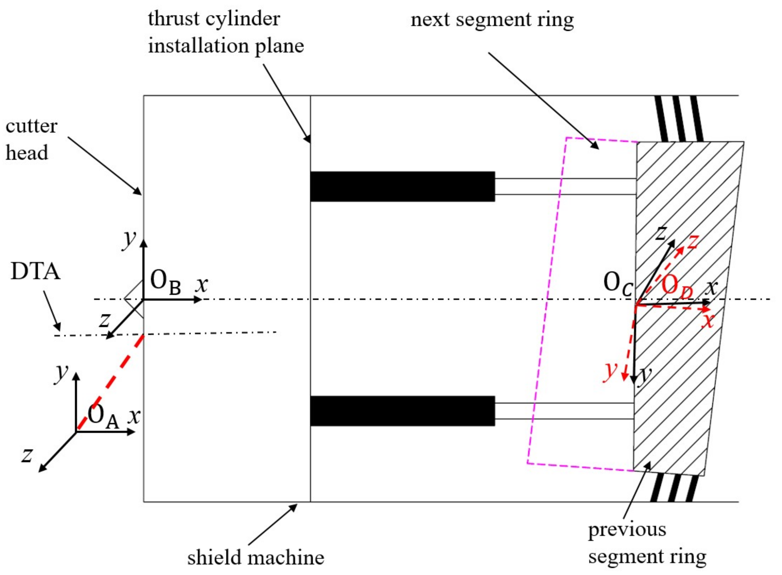
As shown in Figure 2, the shield machine is seen as a cylindrical structure, and the thrust cylinders are installed in the shield machine. The cylinders extend on the side wall of the assembled segment ring during operation, the reaction force given by the segment pushing the shield machine forward. The shield machine will stop boring every working stroke, retract the thrust cylinders, and a new segment ring will be assembled with a reasonable assembly point under the tail shield support. This process will continue until the entire tunnel is completed.
Formed tunnels need to fit the DTA for which construction usually follows the following principles: the shield machine borings along the DTA and the segment assemble for the purpose of adjusting the relative location of the shield machine and segments. Meeting this principle enables both safe construction and the fitting of the actual tunnel to the DTA. The relative location of the shield machine and the segment ring is reflected in the shield tail gap and thrust cylinder stroke difference. Selecting reasonable points to assemble the segment will make the shield tail gap and thrust cylinder stroke difference improved to different degrees, which can prevent the shield machine from squeezing with the segments, and the shield machine can have a larger movement space and better deflection correction ability. The lower cylinder stroke U 3 ( n ) and lower shield tail gap T 3 ( n ) before segment ring assembly and the lower cylinder stroke U 3 ( n + 1 ) and lower shield tail gap T 3 ( n + 1 ) after segment ring assembly are shown in Figure 2.

2.1.2. Universal Shield Segment and Its Assembly Point

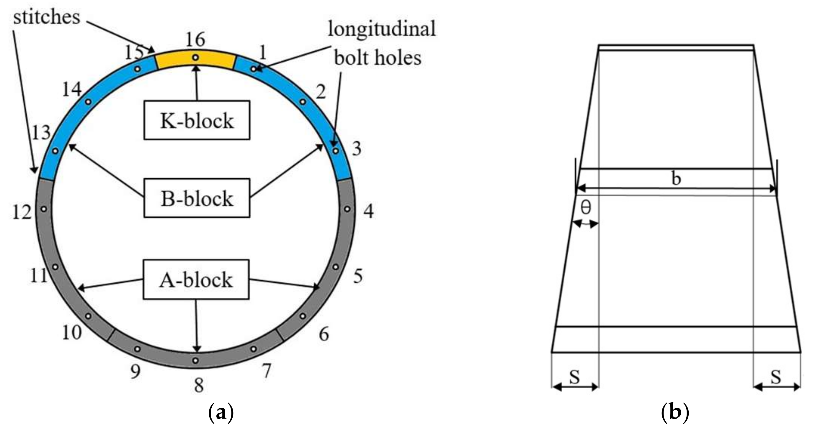
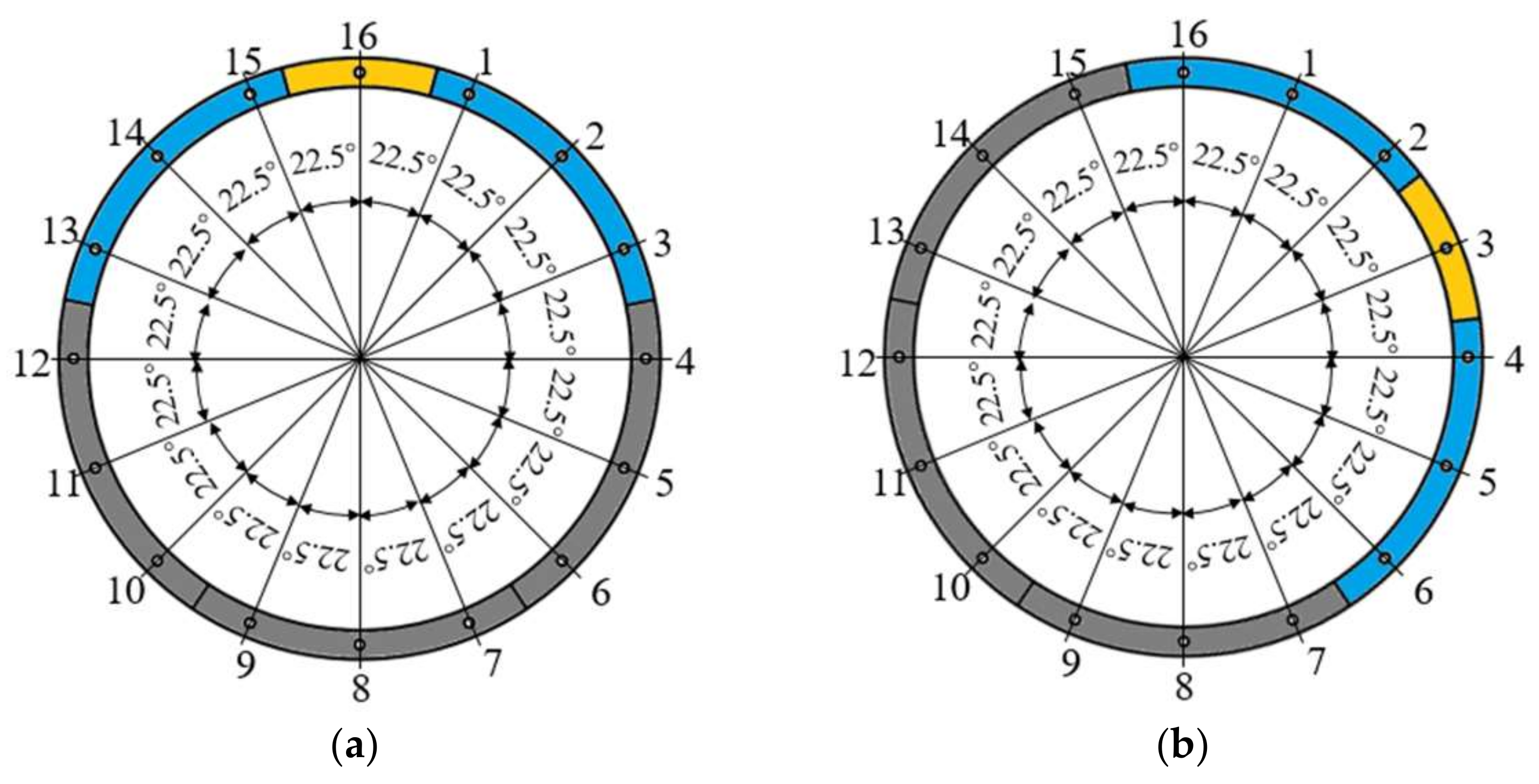
A formed tunnel consists of a large number of lining rings assembled in segments. Figure 3 shows the structure of a 16-points universal shield segment ring. The segment is generally composed of three categories, A, B and K [17]. The segment ring is an isosceles trapezoid from the side view, where S is the unilateral wedge shape of the ring, θ is the wedge angle, b is the central width, and D g is the diameter of outer wall. Due to the wedge shape of ring, the turning of the tunnel and the auxiliary control of the shield machine are realized. Longitudinal bolt holes numbered 1 to 16 are evenly distributed on the end face of the segment ring, and the rings are connected to each other by longitudinal bolts. In this connection, the relative rotation angle between the two adjacent rings cannot be arbitrary but must be an integer multiple of the unit rotation angle (22.5°). The K-block, also called a capping block, is usually assembled last in a ring as the most critical step. The assembly point of the segment is the installation position of the K-block, which is used to describe the rotation angle of the segment ring. As shown in Figure 4a, the K-block is located at the top of the ring; in this case, the assembly point is 16. While in Figure 4b, the K-block rotates 3 × 22.5° clockwise, and the assembly point is 3.
Considering the quality of the tunnel and the difficulty of assembling segments, the lowermost point 8 and the uppermost point 16 are usually not allowed to be selected. In addition, assembling segment rings need to meet the principle of staggered-joint assembly [16], i.e., the stitches between the connecting blocks of two adjacent segment rings need to be staggered. To achieve staggered assembly, the next possible segment assembly point i n + 1 and the previous segment assembly point i n need to satisfy the correspondence in Table 1.

2.2. Optimization Objectives of Assembly Point Selection

2.2.1. Thrust Cylinder Stroke Difference

The thrust cylinders are divided into four groups: upper, lower, left and right. The vertical (top minus bottom) stroke difference and the horizontal (left minus right) stroke difference are important evaluation indexes of the construction conditions. Excessive thrust cylinder stroke discrepancies cause excessive radial component forces to act on the segments, resulting in serious incidents such as shattered segments and uncontrolled shield machine. Choosing different assembly points to assemble the segments will have different adjustments on the thrust cylinder stroke differences, and the effects of the assembly points on the horizontal stroke difference and vertical stroke difference are as follows [33].
U h ( n + 1 ) = U h ( n ) 2 S sin ( 360 ° i n + 1 N )
U v ( n + 1 ) = U v ( n ) + 2 S cos ( 360 ° i n + 1 N )
where U h ( n + 1 ) and U v ( n + 1 ) are the horizontal thrust cylinder stroke difference and the vertical thrust cylinder stroke difference, respectively, after assembling the next segment ring, U h ( n ) and U v ( n ) are the horizontal thrust cylinder stroke difference and the vertical thrust cylinder stroke difference, respectively, before assembling the next segment ring, and N is the total number of assembly points of the segments, taken as 16.

2.2.2. Shield Tail Gap Difference

The assembled segment rings gradually leave the tail shield when the shield machine is tunneling. This requires a certain gap between the inner wall of the tail shield and the outer wall of the assembled segment rings, which is called the “shield tail gap”. When the shield tail gap is too small, the tail shield will squeeze the segments, causing segments to rupture and damage the shield tail seal system [22]. Choosing different segment assembly points to assemble the segments will have different effects on the shield tail gap in the upper, lower, left and right directions. Because the four directions of the shield tail gap are interrelated, to reduce the number of optimization objectives, the horizontal shield tail gap difference T h ( n + 1 ) (left minus right) and the vertical shield tail gap difference T v ( n + 1 ) (upper minus lower) are used as the optimization objectives. The equations for T h ( n + 1 ) and T v ( n + 1 ) are derived separately from the geometric relationships as follows.
T h ( n + 1 ) = T h ( n ) 2 b U h ( n ) D c + 2 b S D g sin ( 360 ° i n + 1 N )
T v ( n + 1 ) = T v ( n ) 2 b U v ( n ) D c 2 b S D g cos ( 360 ° i n + 1 N )
where T h ( n ) and T v ( n ) represent the horizontal and vertical shield tail gap difference before the next segment ring assembly, b is the width of the segment ring, D g is the outer diameter of the segment ring, and D c is the diameter of the cylinder distribution circle, as shown in Figure 2.
In this paper, WCPs refer to U h ( n ) , U v ( n ) , T h ( n ) and T v ( n ) .

2.3. Assembly Point Selection Objective Function

The smaller values of U h ( n + 1 ) , U v ( n + 1 ) , T h ( n + 1 ) and T v ( n + 1 ) indicate the better relative location of the shield machine and segments after assembling. The purpose of selecting the next segment assembly point i n + 1 is to make the four optimization objectives as small as possible. To solve the multi-objective optimization problem of assembly point selection, the weight coefficient transformation method is used to combine the optimization objectives, transforming the multi-objective optimization problem into a single-objective optimization problem and establishing the objective function of assembly point selection (hereafter, objective function), as shown in Equation (5).
min G ( i n + 1 ) = λ h U h 2 ( n + 1 ) + λ v U v 2 ( n + 1 ) + ξ h T h 2 ( n + 1 ) + ξ v T v 2 ( n + 1 ) s . t . 90 U h ( n + 1 ) 90 90 U v ( n + 1 ) 90 90 T h ( n + 1 ) 90 90 T v ( n + 1 ) 90 λ h + λ v + ξ h + ξ v = 1 λ h , λ v , ξ h , ξ v [ 0 , 1 ]
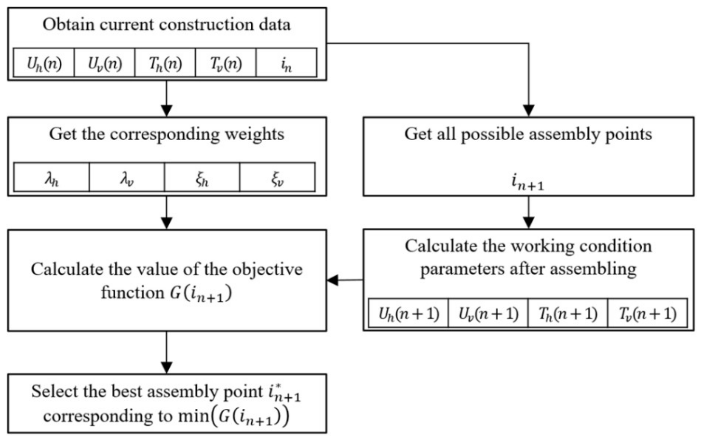
where λ h , λ v , ξ h and ξ v are the corresponding weights of each optimization objective. As mentioned earlier, we have a requirement for the weights: they are adaptively taken with the WCPs. The method of selecting the next segment assembly point is as follows: first, we obtain the current construction data, including the WCPs and the assembly point of the previous segment, and the weights corresponding to the WCPs are determined. Then, all the next segment possible assembly points i n + 1 that meet the staggered-joint assembly are obtained by Table 1. Then i n + 1 are brought into Equations (1)–(5) one by one, and the i n + 1 that minimizes the objective function G ( i n + 1 ) is selected as the best assembly point i n + 1 * of the next segment ring (Figure 5).

3. The Example Dataset Generation

When optimizing the weights of the objective function by genetic algorithm, the correct rate of the assembly points selection using the objective function will be used as an evaluation index. Therefore, the acquisition of the example dataset is crucial. However, it will take about two to three years to generate 1000 groups of data for shield tunneling in actual construction, so we cannot collect enough actual data. Therefore, a simulation-based approach to generate example data is necessary.
The reference factors used by the shield machine drivers in the field to select the next segment assembly point are U h ( n ) , U v ( n ) , T h ( n ) , T v ( n ) and i n ; so the purpose of the simulation is to generate these reference factors as sample data. Then the best assembly point i n + 1 * of the next segment is obtained by the driver’s labeling, and the example data U h ( n ) , U v ( n ) , T h ( n ) , T v ( n ) , i n , i n + 1 * is obtained. Once the location of the shield machine and the previous segment ring is determined, WCPs can be calculated by the homogeneous coordinate transformation and spatial geometry methods. Therefore, the example data generation method can be divided into the generation of the shield machine location, the previous segment ring location based on the Monte Carlo method, calculation of the WCPs and i n and driver labeling.

3.1. Generation of Shield Machine and Previous Segment Ring Location

To describe the relative location between the shield machine and the previous segment ring and to calculate the thrust cylinder stroke and shield tail gap, four coordinate systems were established on the DTA, the shield machine and the previous segment ring, respectively. As shown in Figure 6, the origin of the shield machine coordinate system {B} is on the center point of the cutter head of the shield machine, the origin of the DTA coordinate system {A} is on the DTA, and the origin of the coordinate system {B} is on the y A O A z A plane of the coordinate system {A}. The origin of the coordinate system {C} is on the center point of the front face of the previous segment ring, and the x-axis is perpendicular to the front face, the y-axis is directed to the center of the K-block, and the z-axis is determined by the rules of the right-hand coordinate system. The coordinate system {C} is rotated along the z-axis so that the x-axis coincides with the axis of the previous segment ring, and the coordinate system {D} is obtained.
The value range of each location parameter was determined by the construction specification and engineering experience, including the location of the shield machine relative to the DTA ( x 1 , y 1 , z 1 , α B , β B , γ B ) and the location of the previous segment ring relative to the DTA ( x 2 , y 2 , z 2 , α C , β C , γ C ), and the value range of each location parameter is shown in Table 2.

3.2. The Calculation of Thrust Cylinder Stroke

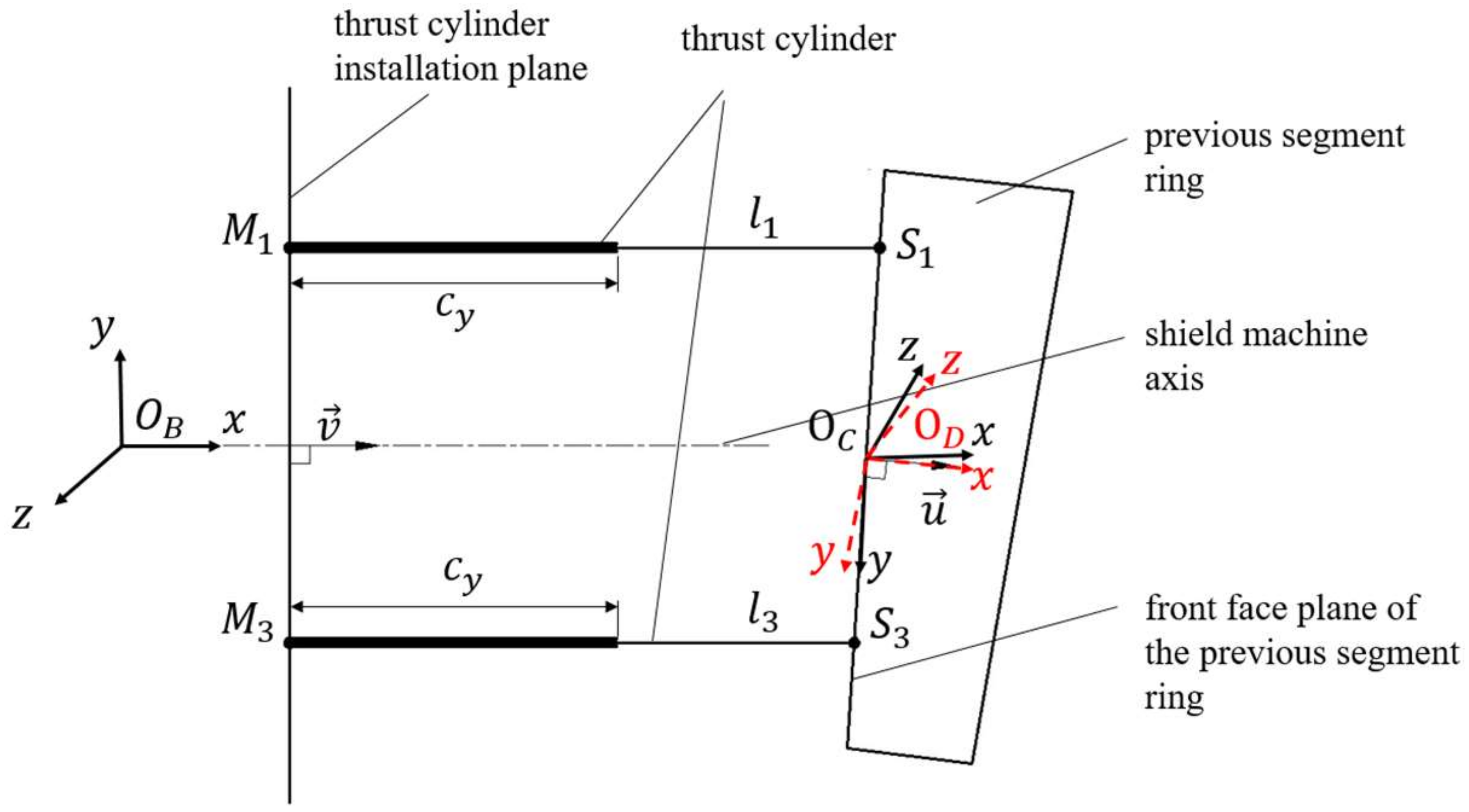
Four thrust cylinders are installed in the shield machine; let the four installation points be M k ( k = 1 , 2 , 3 , 4 ) , respectively. In addition, the intersection points of the thrust cylinder and the previous segment ring are S k ( k = 1 , 2 , 3 , 4 ) . The thrust cylinder stroke can be calculated by calculating the distance between the installation points and the intersection points; the calculation schematic is shown in Figure 7.
It is easy to know that the coordinates of the four thrust cylinder installation points M k B ( k = 1 , 2 , 3 , 4 ) in O B X B Y B Z B , then in the O A X A Y A Z A , the installation points can be expressed as:
M k A = T B A M k B
T B A = c β B c γ B c β B s γ B s β B x 1 s α B s β B c γ B + c α B s γ B s α B s β B s γ B + c α B c γ B s α B c β B y 1 c α B s β B c γ B + s α B s γ B c α B s β B s γ B + s α B c γ B c α B c β B z 1 0 0 0 1
where T B A denotes the homogeneous transformation matrix (HTM) from O B X B Y B Z B to O A X A Y A Z A , c and s represent cosine and sine functions, respectively, x 1 , y 1 , z 1 , α B , β B and γ B are obtained from Section 3.1.
Similarly, the HTM T C A from O C X C Y C Z C to O A X A Y A Z A can be obtained from the location of the previous segment relative to the DTA.
Considering the four thrust cylinders as straight lines l k ( k = 1 , 2 , 3 , 4 ) parallel to the shield machine axis, their direction vector in O A X A Y A Z A can be expressed as:
v A = T B A v B = T B A 1 0 0 1 T
Then the line l k ( k = 1 , 2 , 3 , 4 ) can be expressed as:
M k A P k A = t 1 v A
where P k is any point on the line l k , and t 1 is an arbitrary real number.
In O A X A Y A Z A , the normal vector of the front face of the previous segment ring can be expressed as:
u A = T C A u C = T C A 1 0 0 1 T
where u C is the normal vector of the front face of the previous segment ring in O C X C Y C Z C .
In O A X A Y A Z A , the center point of the front face of the previous segment ring is given by:
O C A = T C A O C C = T C A 0 0 0 1 T
where O C C is the center point of the front face of the previous segment ring in O C X C Y C Z C .
Then the front face plane equation of the previous segment ring can be expressed in O A X A Y A Z A as:
O C A P 5 A u A = 0
where P 5 is any point on the plane.
The intersection points A S k ( k = 1 , 2 , 3 , 4 ) between the thrust cylinder and the front face of the previous segment ring in O A X A Y A Z A can be found by Equations (9) and (12).
Let the length of the thrust cylinder when it is not extended be c y , then the four thrust cylinders (upper, right, lower, left) stroke U k ( n ) ( k = 1 , 2 , 3 , 4 ) can be given by:
U k ( n ) = A M k A S k c y , ( k = 1 , 2 , 3 , 4 )

3.3. The Calculation of Shield Tail Gap

One of the main measurement methods for the shield tail gap is the measurement method with pre-set sensors on the inner wall of the tail shield. By measuring the distance to the outside wall of the segment ring using a laser displacement sensor located on the inner wall of the tail shield, this method achieves automated and accurate measurement of the shield tail gap. Simulating this process, the calculation method of the shield tail gap is proposed.
Figure 8 shows the schematic diagram of the shield tail gap calculation. Pass the four shield tail gap measurement points H k ( k = 1 , 2 , 3 , 4 ) , which are located on the inner wall of the tail shield, make straight lines l 5 and l 6 perpendicular to the axis of the tail shield, and find the intersection points D k ( k = 1 , 2 , 3 , 4 ) of the straight lines with the outer wall of the previous segment ring, then the shield tail gap can be expressed as H k D k .
The outer cylindrical surface of the segment ring is described in O D X D Y D Z D as:
O C D O 6 D × w D = D g 2 w D
where P 6 is any point on the cylindrical surface, O C is the origin of the coordinate system O D X D Y D Z D , w is the direction vector of the axis of the cylindrical surface, and w D = 1 0 0 1 .
The coordinate system O D X D Y D Z D is obtained by rotating the coordinate system O C X C Y C Z C by an angle θ along the z-axis so that the x-axis coincides with the axis of the previous segment ring, so the HTM from O C X C Y C Z C to O D X D Y D Z D can be expressed as:
T C D = c θ s θ 0 0 s θ c θ 0 0 0 0 1 0 0 0 0 1
The coordinates of the shield tail gap measurement point in O B X B Y B Z B are H k B ( k = 1 , 2 , 3 , 4 ) ; then the coordinate in O D X D Y D Z D can be given by:
H k D = H B D H k B
T B D = T 1 B A T C A 1 T C D
where T B D is the HTM from O B X B Y B Z B to O D X D Y D Z D .
In O D X D Y D Z D , the direction vectors t 1 D and t 2 D of l 5 and l 6 can be expressed, respectively, as:
t 1 D = T B D t 1 B = T B D 0 1 0 1
t 2 D = T B D t 2 B = T B D 0 0 1 1
where t 1 B and t 2 B are the direction vectors of l 5 and l 6 in O B X B Y B Z B , respectively.
Then, l 5 and l 6 can be expressed as:
H 1 D P 7 D = k 2 t 1 D
H 2 D P 8 D = k 3 t 2 D
where P 7 and P 8 are any points on the lines l 5 and l 6 , respectively, k 2 and k 3 are arbitrary real numbers.
From Equations (14), (20) and (21), the intersection points D k ( k = 1 , 2 , 3 , 4 ) of the shield tail gap measurement lines and the outer wall of the segment ring in O D X D Y D Z D can be obtained, so the four shield tail gaps can be expressed as:
T k ( n ) = H k D D k D , ( k = 1 , 2 , 3 , 4 )

3.4. Simulation Data Processing

After the simulation has obtained the thrust cylinder stroke and the shield tail gap, the following steps are still required to obtain the sample data.
(1)
Adding noise to simulation data: Because the measurement precision of both the thrust cylinder stroke measurement sensors and the shield tail gap measurement sensors in construction is 1 mm, random errors X are added in the form of Gaussian noise on U k ( n ) and T k ( n ) , respectively, in which X ~ N ( 0 , 1 / 3 ) .
(2)
Calculation and screening of WCPs: U h ( n ) , U v ( n ) , T h ( n ) and T v ( n ) are calculated from U k ( n ) ( k = 1 , 2 , 3 , 4 ) and T k ( n ) ( k = 1 , 2 , 3 , 4 ) . In addition, the range of values of WCPs is determined through engineering experience, as shown in Equation (23):
90 U h ( n ) , U v ( n ) , T h ( n ) , T v ( n ) 90
retaining the set of WCPs that simultaneously satisfy Equation (23). In addition, it should be noted that the previous segment assembly point i n has been determined when generating the previous segment ring location in Section 3.1; so a set of sample data ( U h ( n ) , U v ( n ) , T h ( n ) , T v ( n ) , i n ) can be obtained.

3.5. Data Labeling and Expansion

The sample data were labeled manually by several shield machine drivers. The general principle followed in selecting the assembly point is: When a parameter is poor, i.e., the value is close to the maximum, the assembly point that can improve that parameter to a greater extent will be selected; when both the shield tail gap difference and the thrust cylinder stroke difference are poor, priority will be given to improving the shield tail gap difference. On the basis of following the general principle, these drivers balance the parameters that should be adjusted in a set of sample data, and then through extensive calculations and discussions, the best assembly point i n + 1 * is selected as the label. Table 3 shows a set of manually labeled data ( U h ( n ) , U v ( n ) , T h ( n ) , T v ( n ) , i n , i n + 1 * ).
As we know, the genetic algorithm requires sufficient example data to optimize the weights in each interval, but a sufficient amount of sample data labeled manually by shield machine drivers would take a huge amount of time and effort. To solve this problem, a data augmentation method is proposed.
From Equations (1)–(4), it can be seen that the adjustment of the WCPs is opposite for the symmetrically positioned assembly points; so when the WCPs are symmetrically transformed, the assembly points of the previous segment and the next segment should also be symmetrically transformed to achieve the same parameter optimization effect. The thrust cylinder stroke and shield tail gap are converted horizontally, vertically and diagonally, and the segment assembly points are changed to the corresponding transformed points according to the point distribution shown in Figure 3. Table 3 shows the results of the expansion of a set of data, as well as the results of the adjustment of the WCPs (when S = 19 , b = 1500 , D c = 5700 , D g = 6000 ).
This expansion method generates data with the same optimization-focused parameters as the original data. After the drivers labeled the sample data and data expansion, we finally obtained 11570 sets of example data that were uniformly distributed in the working condition.

4. Genetic Algorithm-Based Weights Optimization

For the purpose of achieving adaptive and reasonable values of the weights λ h , λ v , ξ h and ξ v , we divide the working condition into multiple intervals and use genetic algorithm to optimize weights within each interval.

4.1. Divide the Working Condition into Intervals

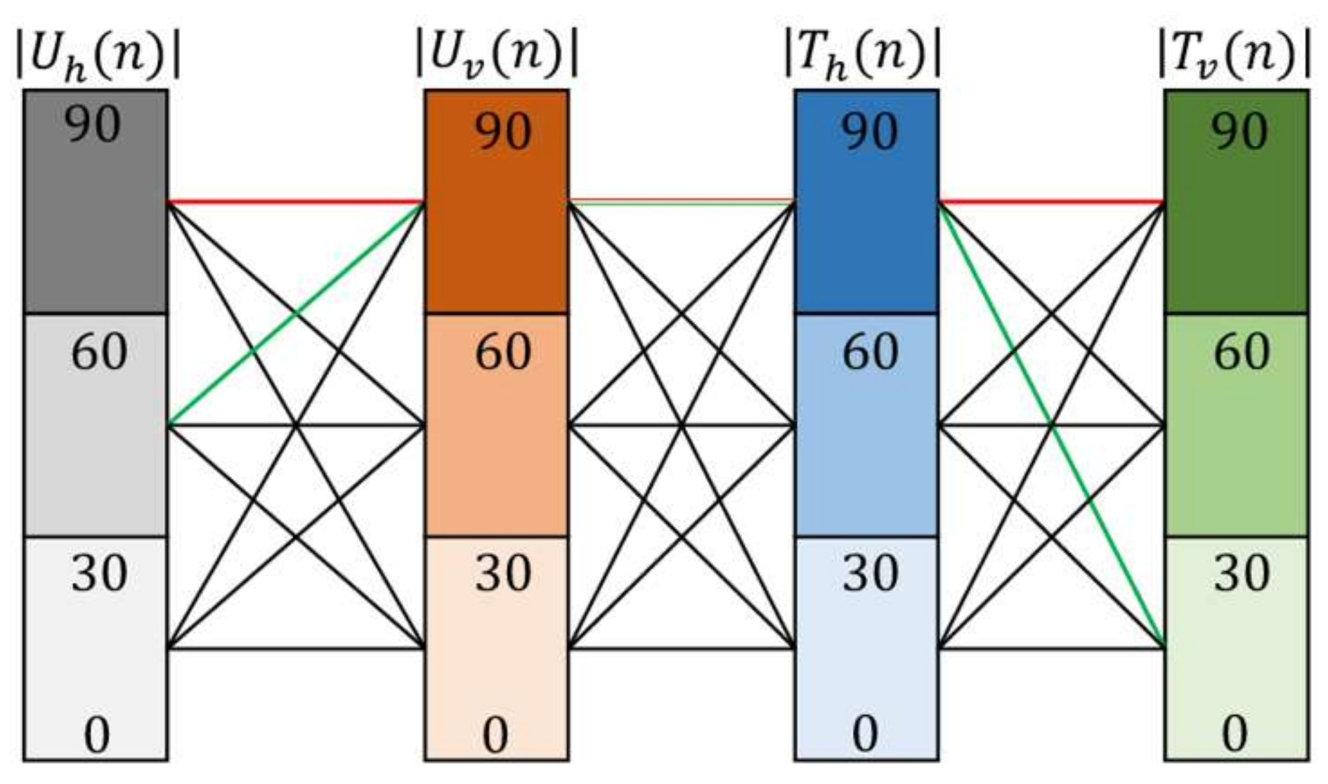
WCPs with the same absolute value can use the same weights; so the absolute values of WCPs are used as indicators to divide the working conditions into multiple intervals. The evaluation of the WCPs in construction is usually divided into three categories of good, medium and poor. So we divide U h ( n ) , U v ( n ) , T h ( n ) and T v ( n ) into three categories each and use 30 and 60 as interval boundary values, respectively, based on engineering experience. The categories of different parameters are combined to obtain 81 intervals. Figure 9 shows the partitioning method, and the categories connected by the red and green lines represent the two intervals, respectively.

4.2. Genetic Algorithm Design

4.2.1. Chromosome Encoding

When executing genetic algorithms, encoding is required to transform feasible solutions into chromosomes that can perform genetic operations. Binary encoding, with its simplicity and ease of use, is the most common encoding method for genetic algorithm [34,35]; so we use a binary encoding method in this work.
The range of values of the objective function weights is [0, 1], and the precision is set to 0.01. The number of genes m of the chromosome is determined by Equation (24).
2 m 1 < ( 1 0 ) × 10 2 2 m 1
It can be calculated that m = 7 . As shown in Figure 10, the chromosome containing 28 genes represents the information of 4 weights, one weight for each 7 genes, e.g., genes 1, 5, 9, 13, 17, 21 and 25 together represent λ h .

4.2.2. Genetic Operations

Genetic operations include selection, crossover and mutation operations, which are described as follows.
(a)
Selection: According to the fitness value, chromosomes are selected by the Roulette Wheel Selection. In addition, the elite retention strategy is used to add the best chromosome from the previous population to the next, to protect the optimal chromosome structure and improve the convergence of the algorithm.
(b)
Crossover: A crossover operation is to simulate a genetic recombination in biological genetic and evolutionary processes. A single-point crossover is used to randomly select a crossover point and swap the genes behind the crossover point to form two new chromosomes. Whether the crossover operation is executed or not is determined by the crossover probability P c .
(c)
Mutation: The mutation operation is performed to maintain the diversity of the population and prevent the problem from falling into local convergence. For the selected chromosomes, a mutation point is randomly selected, and the genes at the mutation point are converted between zero and one according to the mutation probability P m .

4.2.3. Fitness Value

The four weights λ h j , λ v j , ξ h j and ξ v j ( j = 1 , 2 , 81 ) represented by the chromosome are brought into Equation (5) to obtain the intra-interval objective function, which is used to select the assembly points of the example data in the interval. The selection results are compared with the labels, and the correct rate p j is used as the fitness value.
As the number of iterations of the genetic algorithm increases, the difference in fitness between chromosomes becomes smaller to enhance the selection ability of the optimal chromosome. The Fitness Scaling Transform is needed to obtain the optimal individual as early as possible. The Fitness Scaling Transform is shown in Equations (25) and (26) [36].
f t = a f + b
a = ( C 1 ) f a v g f max f a v g b = ( f max C f a v g ) f a v g f max f a v g
where f t is the transformed fitness of a chromosome, f is the original fitness of the chromosome, a and b are coefficients, f a v g is the average fitness value in the population, f max is the maximum fitness in the population, f min is the minimum fitness in the population, and C is any positive real number in the interval [1.2, 2].

4.2.4. Operation Process of the Genetic Algorithm

The genetic algorithm is used to optimize the weights in each interval. The flow of the genetic algorithm is shown in Figure 11.
The steps of the proposed algorithm are as follows:
Step 1: Working condition partition.
Divide the working conditions into 81 intervals, and we refer to each interval as Ω j (j = 1,2, … 81). Correspondingly, the example dataset is divided into 81 intervals, too.
Step 2: Population initialization.
For the interval Ω j (j = 1,2, … 81), initialize the genetic algorithm population, and M chromosomes are obtained.
Step 3: Fitness value calculation.
The weights of the chromosome representation are brought into the objective function to select the assembly points of the example data, and the assembly point selection correct rate is used as the fitness value of the chromosome.
Step 4: Genetic operations.
  • Select M 1 chromosomes based on the fitness value using Roulette Wheel Selection.
  • Randomly select two parent chromosomes to perform one-point crossover with probability P c .
  • Randomly select a point to perform a one-point mutation with probability P m .
  • Keep the best chromosome (the elite) of the previous population to the next, and a new population containing M chromosomes is obtained.
Step 5: Iteration termination judgment.
Repeat steps 3–4 until the number of iterations reaches MaxIter, and the optimization of the weights of the interval Ω j is completed.
Step 6: Complete optimization of all intervals.
Go back to Step 2 until the optimization of the weights of all intervals is completed, and then generate the optimal weights { ( λ h j * , λ v j * , ξ h j * , ξ v j * ) , j = 1 , 2 , 81 } and the total correct rate of selected assembly points P*. The total correct rate P* is calculated from Equation (27)
P * = j = 1 81 p j · n d j N D
where p j is the correct rate in Ω j , n d j denotes the number of examples in Ω j and N D denotes the total number of examples.
The parameters used in the genetic algorithm are described in Table 4.

5. Results and Discussion

5.1. Weights Optimization and Validation

To evaluate the effectiveness of the proposed approach, 70% of the 11,570 example data is used for training and 30% for testing. Moreover, the parameter values of the genetic algorithm are listed in Table 4. The proposed genetic algorithm is programmed in Python, and the program runs on a computer with an environment of 6136 CPU, 3.0 GHZ frequency and 32 GB memory.
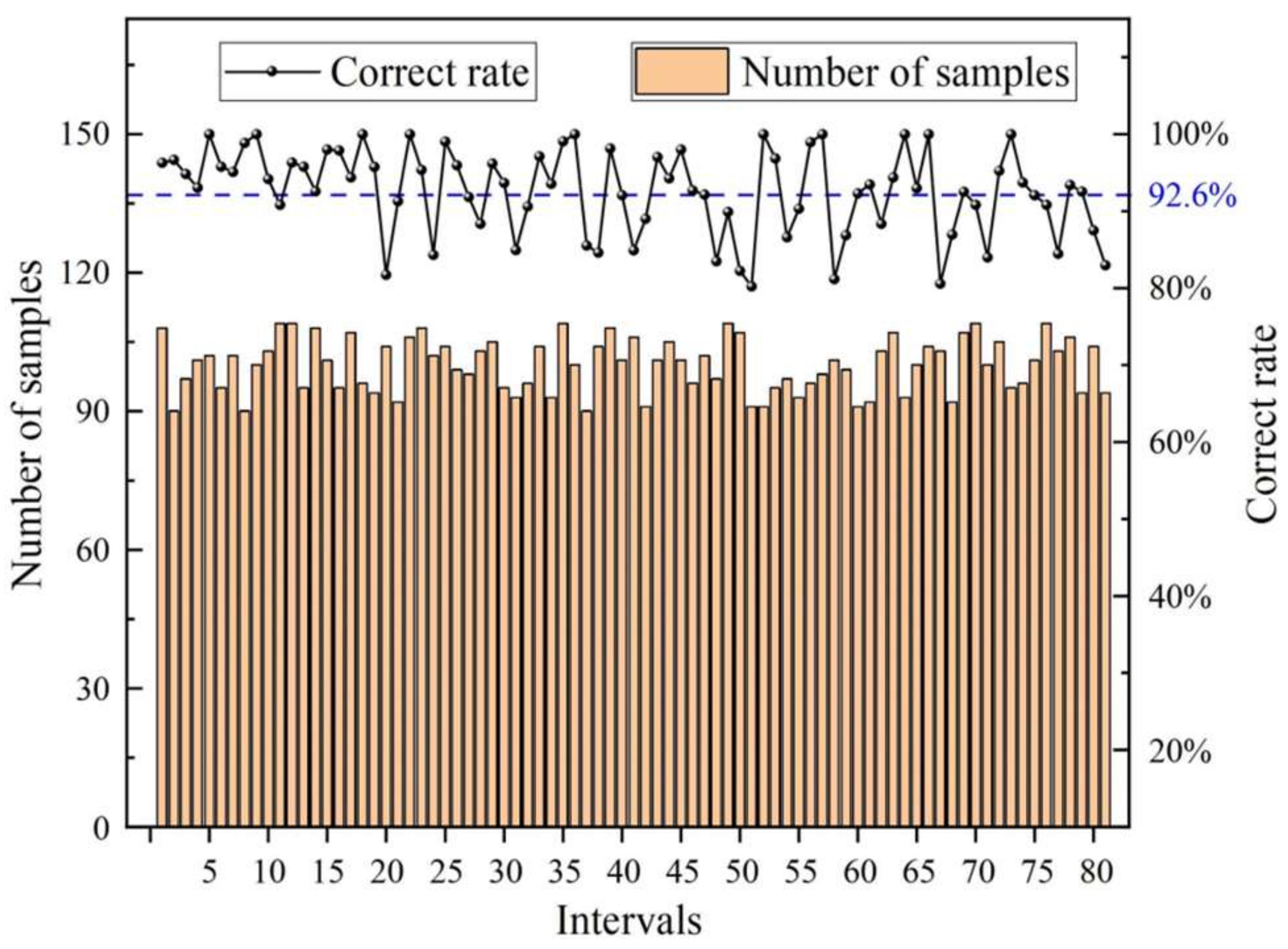
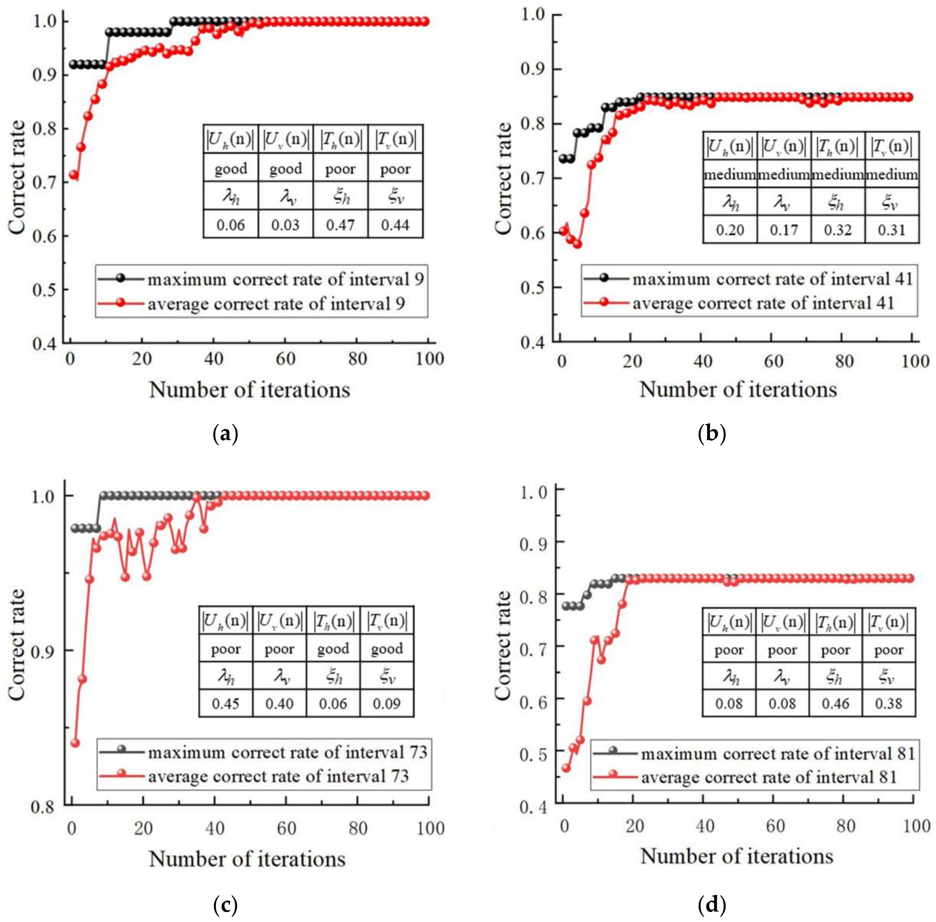
The genetic algorithm optimizes the weights in 81 intervals, and the objective function is used to select the assembly points with a total correct rate of 92.6%. The training correct rate and examples of each interval are shown in Figure 12, and it can be seen that the examples are uniformly distributed in each interval, and the example size of each interval is within the range of [90, 110], which can provide confidence in the correct rate of the point selection and the optimized weights. The correct rate of all intervals is above 80%, but the correct rate of certain intervals is high, such as interval 9, 73, etc. All reach 100%, and the correct rate of the certain interval is low, such as 80.2% for interval 51. This is because when the drivers make the labels, the degree of focus on optimizing the different WCPs is continuously changing, and the weights should theoretically change continuously. However, we divide the whole working condition into 81 intervals with defined interval boundary values and share the same weights within the interval. This approach leads to assembly point selection results for some transition data around interval boundary values that do not match the labels, resulting in a slightly lower correct rate in certain intervals. However, in practical engineering, these transition data often have two or even more optional assembly points. Even though the objective function selected points are different from the labels, they are still available.
Figure 13 shows the genetic algorithm iteration diagrams of the four intervals 9, 41, 73 and 81. From the four iteration diagrams, it can be seen that the maximum assembly point selection correct rate (the maximum correct rate in a population) increases with the number of iterations and remains stable after reaching the maximum correct rate. In addition, the average correct rate (the average correct rate of a population) also gradually approaches the maximum correct rate of assembly point selection with the increase of the number of iterations and finally reaches convergence, which proves the convergence of the algorithm. It can also be noted that the relatively small number of steps and faster convergence of the genetic algorithm is due to the fact that a number of weights can be used as optimal weights to achieve the selection of best assembly point from four to five possible assembly points.
Interval 9 corresponds to working conditions where U h ( n ) and U v ( n ) are good, while T h ( n ) and T v ( n ) are poor, and the weights are 0.06, 0.03, 0.47 and 0.44, respectively. Interval 73 corresponds to working conditions where U h ( n ) and U v ( n ) are poor, while T h ( n ) and T v ( n ) are good, and the optimized weights are 0.45, 0.40, 0.06 and 0.09, respectively. The optimization results from the two intervals show that the genetic algorithm assigns larger weights to the poorer WCPs. Interval 41 corresponds to working conditions where U h ( n ) , U v ( n ) , T h ( n ) and T v ( n ) are all medium, and the weights are 0.20, 0.17, 0.32 and 0.31, respectively. In addition, interval 81 corresponds to working conditions where U h ( n ) , U v ( n ) , T h ( n ) and T v ( n ) are all poor, and the optimized weights are 0.08, 0.08, 0.46 and 0.38, respectively. The optimization results from intervals 41 and 81 show a preference for adjusting the shield tail gap, and the preference is more obvious when the shield tail gap is poor. The optimization results of the weights are consistent with the expectation, which proves the reliability of the algorithm.
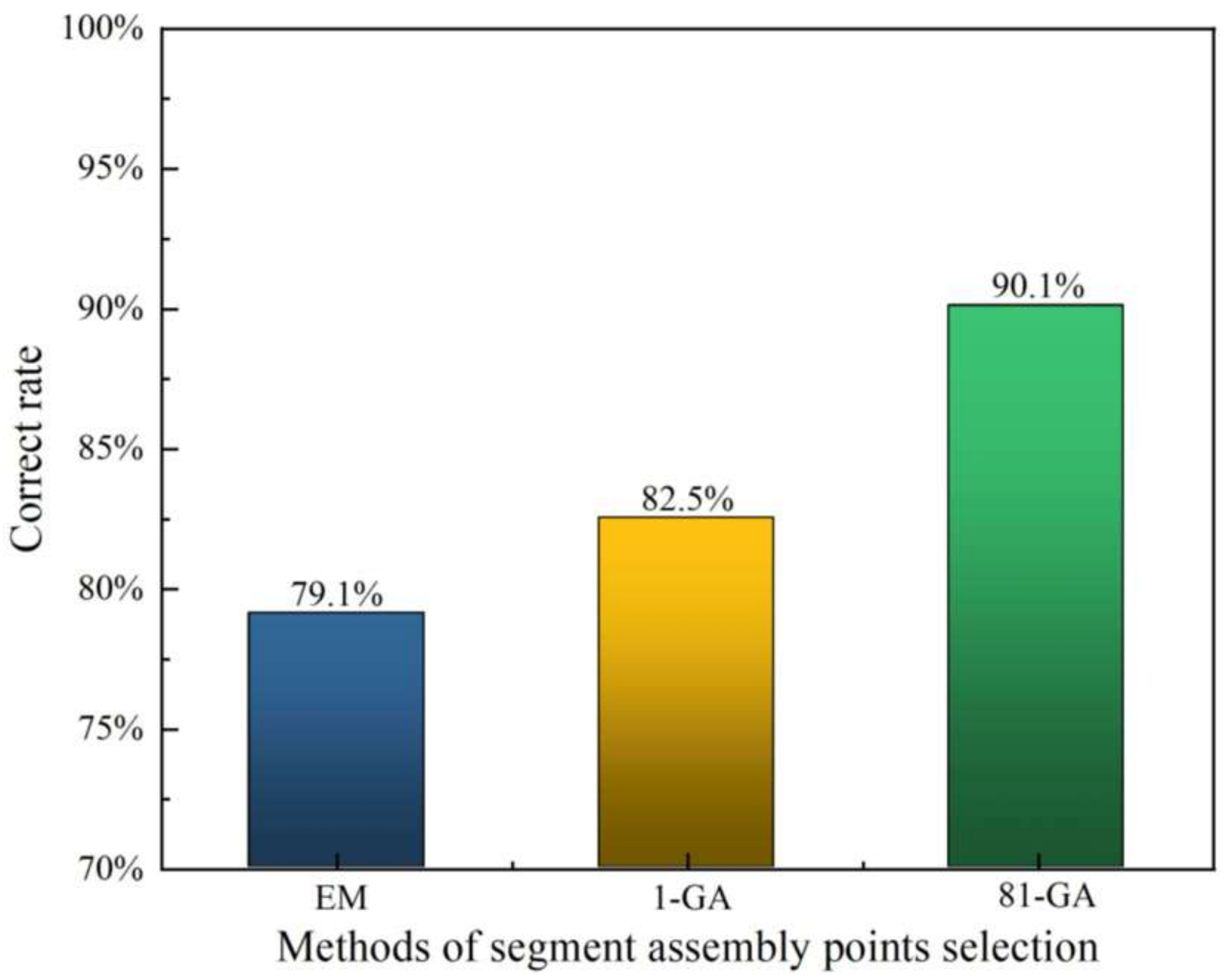
The intelligent selection method of segment assembly points obtained by dividing the working conditions into 81 intervals and optimizing the weights by genetic algorithm in each interval is called 81-GA. Other than this, the method 1-GA was obtained by using the genetic algorithm to optimize the weights without partitioning, and based on the experience of shield machine drivers, the empirical method (EM) was established with λ h : λ v : ξ h : ξ v = 1 : 1 : 2 : 2 . The above three methods were tested with test data. Figure 14 shows the testing correct rate of the above methods.
It can be seen that 1-GA has a correct rate 3.4% higher than EM, which shows that the genetic algorithm optimizes the weights with superiority, and the empirical taking of the weights has certain reasonableness (the accuracy reaches 79.1%). Moreover, 81-GA has a 7.6% higher correct rate than 1-GA, which shows that dividing the working condition into intervals and adaptive change of the weights with the WCPs can make the weights match the working condition better, and the assembly point selection correct rate is higher. The 90.6% correct rate of the test set reflects the high reliability of the 81-GA.

5.2. Site Applications

The method 81-GA was applied on site from Tongle Station to Fengqing Station of Zhengzhou Railway Line 8 in China. When actually selecting the segment assembly points, the shield machine driver could not guarantee the reasonableness of the selected points for each ring due to the shortage of time, incomplete consideration and personal negligence. So, two drivers with sufficient experience were invited to check the points for rings 1~21 of the right line and rings 80~90 of the left line after abundant calculations and discussions, and the most reasonable selectable points were given (some rings have two optional assembly points). In addition, the next segment assembly points of these 32 sets of data were selected using the 81-GA method, and the comparison of 81-GA selected points with the actual points and the driver checked points is shown in Table 5.
As can be seen from the table, the consistency between the actual points and the driver checked points is only 78.1% (25/32), indicating that the actual selection of assembly points by drivers in construction will be greatly influenced by the environment, time and human factors, resulting in the unreasonable selection of some assembly points. The consistency between the points selected by 81-GA and the driver checked points is closer, reaching 90.6% (29/32), indicating that the assembly points selected by the proposed method are more reasonable than the actual points, which proves the reliability of the method. It can be conjectured that 81-GA has the ability to guide the selection of points in the construction site.

6. Conclusions

This paper presents a method to select universal shield segment assembly points. Through the study of example data, this method can automatically select the best assembly point of the next segment ring based on WCPs and previous assembly points. This method eliminates the need for manual selection of assembly points and provides a higher accuracy rate. The following conclusions can be drawn in this study.
  • To establish the intelligent selection method of assembly points, the factors influencing the selection of the assembly points were analyzed, and an objective function for the selection of the universal shield segment assembly point was designed. The working conditions were divided into 81 intervals, and the genetic algorithm was used to optimize the weights of the objective function.
  • Because it is difficult to obtain sufficient example data to optimize the weights, this paper also proposed a calculation method of WCPs based on homogeneous coordinate transformation and spatial analytic geometry methods. The Monte Carlo method is used to generate any required amount of data.
  • The genetic algorithm obtained 92.6% accuracy on the training set when optimizing the weights. The genetic algorithm assigned larger weights to worse WCPs, reflecting the tendency to adjust the worse parameters as much as possible, and overall assigned larger weights to the shield tail gap, reflecting the tendency to preferentially adjust the shield tail gap. Moreover, the preference is more obvious when the shield tail gap is poor.
  • The results on the test data show that the proposed method of assembly point selection can reach a 90.1% correct rate. In addition, the intelligent selection method of assembly point was applied on Line 8 of the Zhengzhou rail transit in China, and the correct rate of assembly points selection reached 90.6%, which is 12.5% higher than the correct rate of actual assembly point selection in the site, indicating that the proposed method has higher accuracy than the actual assembly point selection on site.
Furthermore, as future work, the empirically selected interval boundary values can also be optimized, and the case of more subdivisions of the working condition will be explored.

Author Contributions

Conceptualization, R.L. and G.Z.; methodology, R.L. and J.H.; software, R.L.; validation, R.L. and J.H.; investigation, R.L. and D.Z.; data curation, D.P.; writing—original draft preparation, R.L. and J.H.; writing—review and editing, R.L. and D.Z.; supervision, G.Z.; funding acquisition, G.Z. All authors have read and agreed to the published version of the manuscript.

Funding

This research was funded by the National Key Research and Development Plan of China, grant number 2020YFB1713900.

Institutional Review Board Statement

Not applicable.

Informed Consent Statement

Not applicable.

Data Availability Statement

Not applicable.

Conflicts of Interest

The authors declare no conflict of interest.

References

  1. Shen, S.L.; Xu, Y.S. Numerical evaluation of land subsidence induced by groundwater pumping in Shanghai. Can. Geotech. J. 2011, 48, 1378–1392. [Google Scholar] [CrossRef]
  2. Su, W.L.; Li, X.G.; Jin, D.L.; Yang, Y.; Qin, R.C.; Wang, X.Y. Analysis and prediction of TBM disc cutter wear when tunneling in hard rock strata: A case study of a metro tunnel excavation in Shenzhen, China. Wear 2020, 446, 203190. [Google Scholar] [CrossRef]
  3. Yagiz, S. Utilizing rock mass properties for predicting TBM performance in hard rock condition. Tunn. Undergr. Space Technol. 2008, 23, 326–339. [Google Scholar] [CrossRef]
  4. Yang, F.J.; Zhou, H.; Zhang, C.Q.; Lu, J.J.; Lu, X.J.; Geng, Y.J. An analysis method for evaluating the safety of pressure water conveyance tunnel in argillaceous sandstone under water-weakening conditions. Tunn. Undergr. Space Technol. 2020, 97, 103264. [Google Scholar] [CrossRef]
  5. Ye, F.; Qin, N.; Liang, X.; Ouyang, A.H.; Qin, Z.; Su, E.J. Analyses of the defects in highway tunnels in China. Tunn. Undergr. Space Technol. 2021, 107, 103658. [Google Scholar] [CrossRef]
  6. Zhang, J.W.; Lin, Y.; Chen, Y.Y.; Li, X. Deformation Behavior of Shield Segment Joint Controlled by Bolt and Positioning Tenon. Arab. J. Sci. Eng. 2021, 46, 11241–11251. [Google Scholar] [CrossRef]
  7. Nie, H.B.; Gu, S.C. Ultimate Bearing Capacity Analysis of CFRP-Strengthened Shield Segments Using Bonding Slip Behavior Experiments. Materials 2020, 13, 4200. [Google Scholar] [CrossRef]
  8. Zhang, J.W.; Guo, S.C.; Chen, Y.Y. Mechanical behavior of sealed waterproof for shield tunnel segment joint under different assembling ellipticity. Sci. Prog. 2021, 104, 0036850420987044. [Google Scholar] [CrossRef]
  9. Zhang, W.J.; Koizumi, A. Behavior of composite segment for shield tunnel. Tunn. Undergr. Space Technol. 2010, 25, 325–332. [Google Scholar] [CrossRef]
  10. Wang, S.M.; Wang, X.M.; Chen, B.; Fu, Y.B.; Jian, Y.Q.; Lu, X.X. Critical state analysis of instability of shield tunnel segment lining. Tunn. Undergr. Space Technol. 2020, 96, 103180. [Google Scholar] [CrossRef]
  11. Jin, H.; Su, J.; Zhao, C. Relationship between Invert-Filling Disengaging and Deformation of Shield Tunnel Using Staggered Assembled Segment. Ksce J. Civ. Eng. 2022, 26, 1966–1977. [Google Scholar] [CrossRef]
  12. Luo, H.B.; Li, L.H.; Chen, K. Parametric modeling for detailed typesetting and deviation correction in shield tunneling construction. Autom. Constr. 2022, 134, 101006. [Google Scholar] [CrossRef]
  13. Wu, C.; Liu, X.J.; Wang, L.P.; Wang, J.S. Dimension optimization of an orientation fine-tuning manipulator for segment assembly robots in shield tunneling machines. Autom. Constr. 2011, 20, 353–359. [Google Scholar] [CrossRef]
  14. Thomas, K.; Günther, M. A numerical study of the effect of soil and grout material properties and cover depth in shield tunnelling. Comput. Geotech. 2006, 33, 234–247. [Google Scholar]
  15. Tomasz, M.; Damian, B.; Joanna, N. Seismic vulnerability of a soil-steel composite tunnel—Norway Tolpinrud Railway Tunnel Case Study. Tunn. Undergr. Space Technol. 2021, 110, 103808. [Google Scholar] [CrossRef]
  16. Zhu, X.; Bao, T.F.; Yu, H.; Zhao, J.L. Utilizing Building Information Modeling and Visual Programming for Segment Design and Composition. J. Comput. Civ. Eng. 2020, 34, 04020024. [Google Scholar] [CrossRef]
  17. Zhou, Y.; Wang, Y.; Ding, L.Y.; Love, P.E.D. Utilizing IFC for shield segment assembly in underground tunneling. Autom. Constr. 2018, 93, 178–191. [Google Scholar] [CrossRef]
  18. Hu, M.; Wu, F.F. Improved multi-classes SVM and application in ring-key position selection in tunnels. In Proceedings of the International Conference on Machine Learning and Cybernetics, Baoding, China, 12–15 July 2009. [Google Scholar]
  19. Song, R.H. Development of Software for Composition and Dynamic Deviation Correction of Universal Segments for Shield Tunnel. Master’s Thesis, Shanghai Jiao Tong University, Shanghai, China, 2008. [Google Scholar]
  20. Hu, C.M.; Zhang, W.C.; Mei, Y.; Lu, Z.Y. Calculation of jack stroke difference range and advancing control of shield machine under known point position of universal ring segment. China Railw. Sci. 2015, 36, 51–57. (In Chinese) [Google Scholar]
  21. Liu, F.H. Study on the Composition and Ring Selection Technology of Universal Segment for Shield-Driven Tunnels. Master’s Thesis, Tongji University, Shanghai, China, 2007. [Google Scholar]
  22. Zhang, W.C.; Zhang, J.; Yan, J.R.; Zhu, Y.H. Selection of the Key Segment Position for Trapezoidal Tapered Rings and Calculation of the Range of Jack Stroke Differences with a Predetermined Key Segment Position. Adv. Civ. Eng. 2021, 2021, 3606389. [Google Scholar] [CrossRef]
  23. Miao, L. Design and Implementation of Dynamic Layout Algorithm FOR general Wedge Segment of Tunnel. Master’s Thesis, Shijiazhuang Tiedao University, Shijiazhuang, China, 2020. [Google Scholar] [CrossRef]
  24. Zhao, W.B.; Li, Z.C.; Zhang, X.R. Research on Adaptive Segment Selection Algorithm Based on Three Axis Fitting. J. Inf. Eng. Univ. 2017, 18, 379–384. (In Chinese) [Google Scholar]
  25. Khan, S.A.; Mahmood, A. Fuzzy goal programming-based ant colony optimization algorithm for multi-objective topology design of distributed local area networks. Neural Comput. Appl. 2019, 31, 2329–2347. [Google Scholar] [CrossRef]
  26. Zhong, Y.G.; Ai, B. A modified ant colony optimization algorithm for multi-objective assembly line balancing. Soft Comput. 2017, 21, 6881–6894. [Google Scholar] [CrossRef]
  27. Hasanoglu, M.S.; Dolen, M. Multi-objective feasibility enhanced particle swarm optimization. Eng. Optim. 2018, 50, 2013–2037. [Google Scholar] [CrossRef]
  28. Tao, G.W.; Feng, J.C.; Feng, H.B.; Feng, H.; Zhang, K. Reducing Construction Dust Pollution by Planning Construction Site Layout. Buildings 2022, 12, 531. [Google Scholar] [CrossRef]
  29. Wang, X.Y.; Zhu, S.J.; Zeng, Q.; Guo, X.N. Improved multi-objective Hybrid Genetic Algorithm for Shape and Size Optimization of Free-form latticed structures. J. Build. Eng. 2021, 43, 102902. [Google Scholar] [CrossRef]
  30. Elshafei, G.; Vilcekova, S.; Zelenakova, M.; Negm, A.M. An Extensive Study for a Wide Utilization of Green Architecture Parameters in Built Environment Based on Genetic Schemes. Buildings 2021, 11, 507. [Google Scholar] [CrossRef]
  31. Seong, N.C.; Kim, J.H.; Choi, W. Adjustment of Multiple Variables for Optimal Control of Building Energy Performance via a Genetic Algorithm. Buildings 2020, 10, 195. [Google Scholar] [CrossRef]
  32. Stamoulis, M.N.; dos Santos, G.H.; Lenz, W.B.; Tusset, A.M. Genetic Algorithm Applied to Multi-Criteria Selection of Thermal Insulation on Industrial Shed Roof. Buildings 2019, 9, 238. [Google Scholar] [CrossRef] [Green Version]
  33. Yan, J.R.; Zhang, W.C. Study on the calculation of position selection of universal ring segment in shield tunneling construction. Chin. J. Undergr. Space Eng. 2019, 15, 577–582. (In Chinese) [Google Scholar]
  34. Pazooki, M.; Mazinan, A.H. Hybrid fuzzy-based sliding-mode control approach, optimized by genetic algorithm for quadrotor unmanned aerial vehicles. Complex Intell. Syst. 2018, 4, 79–93. [Google Scholar] [CrossRef] [Green Version]
  35. Kwon, N.; Song, K.; Ahn, Y.; Park, M.; Jang, Y.J. Maintenance cost prediction for aging residential buildings based on case-based reasoning and genetic algorithm. J. Build. Eng. 2020, 28, 101006. [Google Scholar] [CrossRef]
  36. Lei, Y.J.; Zhang, S.W. Matlab Genetic Algorithm Toolbox and Applications, 3rd ed.; Xidian University Press: Xi’an, China, 2014; pp. 43–59. [Google Scholar]
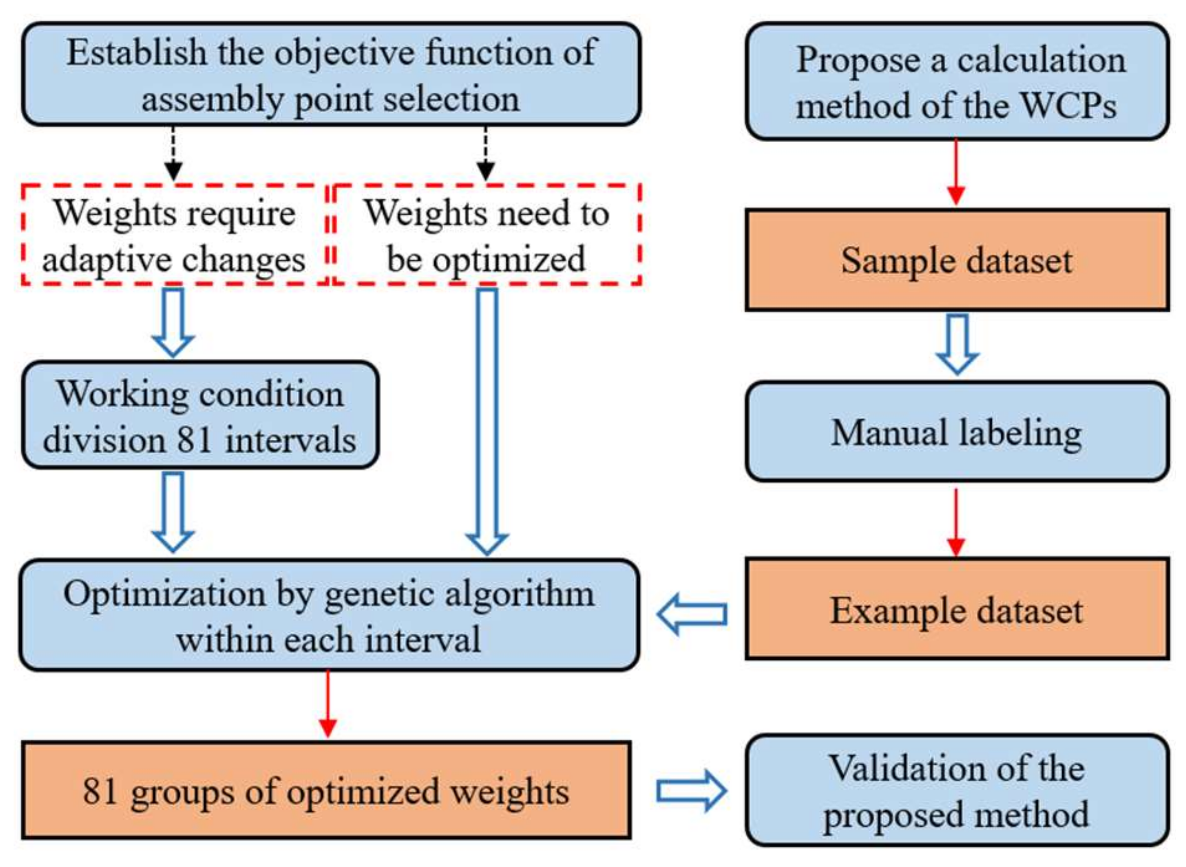
Figure 1. The pipeline of the work.
Applsci 12 06926 g001
Figure 2. Schematic diagram of shield machine and segment ring.
Applsci 12 06926 g002
Figure 3. Universal segment ring structure: (a) front view; (b) side view.
Applsci 12 06926 g003
Figure 4. Assembly points diagram: (a) assembly point 16; (b) assembly point 3.
Applsci 12 06926 g004
Figure 5. Flowchart of selecting the next segment assembly point.
Applsci 12 06926 g005
Figure 6. Coordinate system configuration diagram.
Applsci 12 06926 g006
Figure 7. Schematic diagram of the calculation of the thrust cylinder stroke.
Applsci 12 06926 g007
Figure 8. Schematic diagram of shield tail gap calculation.
Applsci 12 06926 g008
Figure 9. The way working conditions are divided into 81 intervals.
Applsci 12 06926 g009
Figure 10. Structure of chromosome.
Applsci 12 06926 g010
Figure 11. Flowchart of the genetic algorithm.
Applsci 12 06926 g011
Figure 12. Training correct rate of 81 intervals.
Applsci 12 06926 g012
Figure 13. Genetic algorithm iteration diagrams: (a) interval 9 iteration diagram; (b) interval 41 iteration diagram; (c) interval 73 iteration diagram; and (d) interval 81 iteration diagram.
Applsci 12 06926 g013
Figure 14. Correct rate of the test set on different methods.
Applsci 12 06926 g014
Table 1. The correspondence between i n + 1 and i n .
Previous Segment Assembly Point
i n
Next Segment Possible Assembly Point
i n + 1
13691215
2471013
3511141
46912152
5710133
6111414
79121525
91114147
10121525
1113369
121414710
13152511
1436912
151471013
Table 2. Value range of location parameters.
ParametersRange of ValuesParametersRange of Values
x 1 ( mm ) 0 x 2 ( mm ) [6700, 6900]
y 1 ( mm ) [−50, 50] y 2 ( mm ) [−50, 50]
z 1 ( mm ) [−50, 50] z 2 ( mm ) [−50, 50]
α B ( ) [−3, 3] α C ( ) i n 360 16
β B ( ) [−1.5, 1.5] β C ( ) [−3, 3]
γ B ( ) [−1.5, 1.5] γ C ( ) [−3, 3]
Each location parameter is taken randomly within its value range, and the shield machine location and the previous segment ring location are obtained.
Table 3. A set of data expansion results.
Data Types U h ( n ) U v ( n ) T h ( n ) T v ( n ) i n i n + 1 * U h ( n + 1 ) U v ( n + 1 ) T h ( n + 1 ) T v ( n + 1 )
Manually labeled data20701010275353−18
Converted horizontally−2070−1010149−535−3−18
Converted vertically20−7010−10615−35318
Converted diagonally−20−70−10−101015−5−35−318
Table 4. Description of genetic algorithm parameters.
ParametersDescriptionValues
Mnumber of chromosomes in population30
mnumber of genes in a chromosome7
MaxItermaximum number of iterations100
Pcprobability of crossover0.9
Pmprobability of mutation0.05
Table 5. Comparison of 81-GA selected points with actual points and driver calibration points.
Ring
Number
Drivers Checked PointsActual Points81-GA Selected Points
Optional Point 1Optional Point 2Selected PointsIs an Optional PointSelected PointsIs an Optional Point
15 1 5
29 99
37111111
46 3 6
511555
610 1010
712 1212
8107107
95 55
107 77
115252
121371313
135 52
143131313
152 215
1613 1313
171121111
186363
194 44
20126129
21107107
807447
816212 6
827104 7
836212 6
847447
856226
86107710
8715912 15
88714 1
8915121215
90114114
Publisher’s Note: MDPI stays neutral with regard to jurisdictional claims in published maps and institutional affiliations.