This section provides a complete description of the architecture and training process of the proposed DCNN model with the experimental setup and dataset preparation. The proposed plant leaf disease detection model pipeline starts with dataset preparation and ends with model prediction. Python 3.7 programming language and TensorFlow 2.9.1, numpy Version 1.19. 2, matplotlib Version 3.5.2 and OpenCV Version 4.5.5 libraries are used for dataset preparation and DCNN model implementation. Data preparation, preprocessing, model designing and prediction tasks are performed using an HP Z240 workstation with an Intel Core i7 CPU and sixteen gigabytes of random access memory. The training and testing process of the proposed DCNN and existing state-of-the-art techniques were performed using an NVidia DGX-1 deep learning server station. The deep learning server includes two Intel Xeon E5-2694 Version 4 CPUs and eight Tesla P100 GPUs for accelerating the training process of deep neural networks. In subsequent subsections, each phase of the proposed plant leaf disease detection pipeline are discussed in detail. First, the details of the dataset preparation and preprocess are discussed in the next subsection.
3.1. Dataset Preparation and Preprocessing
Diseased and healthy leaf images of various plants were collected from different standard open data repositories [
9,
35,
36,
37,
38]. Sixteen different plant species were used to create the plant leaf disease dataset. Each plant contains healthy and the most common disease classes in the dataset. There are 58 different classes of plant leaves, and 1 no-leaves class is present in the dataset. The collected original dataset contains 61,459 plant leaves and no-leaves images. The list of plant names with the healthy and disease classes of the proposed dataset is shown in
Table 2.
To create an even number of images in each class, data augmentation techniques were introduced. Additionally, the data augmentation techniques can increase the dataset size and reduce the overfitting during the training process of the model by adding some augmented images to the training dataset. The BIM, DCGAN and NST augmentation techniques were used to produce the augmented images in the dataset. The BIM augmentation techniques consist of image cropping, flipping, PCA color augmentation, rotation and scaling. The PCA color augmentation technique alters the intensity of the color channels using the principal component of the pixels [
11]. Additionally, the image cropping, flipping, rotation and scaling techniques create augmented images by changing the color and position of the input images. There are 36,541 augmented images created by the BIM augmentation technique in the dataset.
DCGANs create augmented images that resemble the training data. The DCGAN consists of two DCNN networks, such as generator DCNN and discriminator DCNN. The generator DCNN network takes a vector of random noise and up-samples it to the training data. On the other hand, the discriminator DCNN learns to classify the real and generated images [
33]. The DCGAN network was trained in the graphics processing units with training epochs of 10,000 and a mini-batch size of 64. There are 32,000 augmented images created by the DCGAN augmentation technique in the dataset. NST is another image generation technique using deep learning techniques. A modified VGG19 network was used to develop the NST augmentation model in this research. The NST model was trained with 5000 epochs on the deep learning server system. The NST models require two different input images to generate an augmented output image, such as the content image and the style reference image. At first, the content image contains the essential features to be added to the output image. Second, the style reference image contains style patterns to apply to the output image. To generate the output image, the NST augmentation model applies the style features of the style image to the content image. The NST augmentation technique creates 17,500 augmented images in the dataset. Finally, The BIM, DCGAN and NST techniques were created for the augmented images to balance the data counts in each class of the dataset. The proposed dataset is named the PlantDisease59 dataset. These augmentation techniques increased the number of images in the dataset from 61,459 to 147,500 images. Additionally, the size of individual classes increased to 2500 images in each. Leaf images on the PlantDisease59 dataset were captured in the face-up direction.
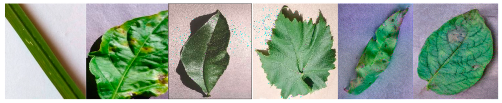
Figure 1 shows the sample augmented images generated by the BIM, DCGAN and NST techniques.
The first two images in
Figure 1 were created using BIM techniques. The third and fourth leaf images in
Figure 1 were created using the DCGAN augmentation technique. The last two sample images in
Figure 1 were generated using the NST technique. The random selection technique was used to select the images for training, validation and testing from the PlantDisease59 dataset.
Table 3 illustrates the number of images in the training, validation and testing dataset.
The design and development of the Proposed DCNN model for plant leaf disease detection using the hyperparameter tuning techniques and the PlantDisease59 dataset are discussed in the following subsection.
3.2. Model Design
In this section, a DCNN model for diagnosing plant leaf diseases using the PlantDisease59 dataset is proposed. Several DCNN models with different numbers and sizes of convolutional (Conv) and pooling layers were developed, and their performance is compared. The number of Conv layers varies from three to eight in different DCNN models. At maximum, the 14-layered deep convolutional neural network (14-DCNN) gives better training performance than other developed models. Five convolutional and five max-pooling layers were used to develop the proposed 14-DCNN model. The input images of the 14-DCNN are given into the first two-dimensional Conv layer. The dimension of the Conv layer output can be calculated using Equation (1):
The input width (
) and height (
) of the first convolutional layer are 128 and 128 respectively. Additionally, the
,
and
represent the width, height and channels of the kernel filter of the convolutional layer. The stride (
) value of this Conv layer is one. The first max-pooling layer was introduced to reduce the dimension of the first Conv layer output from 126, 126, 4 to 63, 63, 4 values. The dimension of the max-pooling layer output was calculated using Equation (2):
The and represent the width, height and channels of input n, respectively. Additionally, the , and represent the width, height and channels of the filter () in the max-pooling layer. The output of the first max-pooling layer is given as an input of the second Conv layer.
Likewise, the second Conv layer uses the filter sizes of 16, 3, 3 values to extract the features from the data. The output size of the second Conv layer is 61, 61, 16 values. The second max-pooling layer reduces the output data size of the second Conv layer from 61, 61, 16 to 30, 30, 16 with the filter size of 2, 2 values. The third Conv layer was introduced after the second max-pooling layer. It extracts more features from the input data using the 32, 3, 3 size kernel and produces the 28, 28, 32 sized output data. The third max-pooling layer was used to reduce the size of the output data from the third Conv layer with 2, 2 sized kernels. It reduces the size of the data to 14, 14, 32 values from 28, 28, 32 values. Additionally, the fourth Conv layer uses the 64, 3, 3 sized kernels to extract the additional features from the third pooled data and generates the output data with the size of 12, 12, 64 values from the input size of 14, 14, 32 values. In addition, the fourth max pooling layer has a filter size of 2, 2 matrices and stride value of 1 step. The fourth max-pooling layer reduces the size from 12, 12, 64 values to 6, 6, 64 values. The fifth Conv layer was introduced with a filter size of 128, 3, 3 matrices. The size of the input matrix is 6, 6, 64 and the output size of the fifth Conv layer is 4, 4, 128 matrices. After the fifth Conv layer, the fifth pooing layer was used with max-pooling function and stride value of 1 step. The input size of the fifth max-pooling layer is 4, 4, 128 values, and the output size is 2, 2, 128 values. It uses the single-step stride values to apply the kernel to the input data from the fifth Conv layer. The
ReLu activation function was used on all the above Conv layers. The
ReLu activation function was performed by using Equation (3).
Moreover, the flatten layer was introduced after the fifth convolutional and pooling layer. It reduces the three-dimensional data to one-dimensional data for a traditional neural network approach. The flatten layer converts the output of the fifth max-pooling layer from 2, 2, 128 values to 512 values. The first dense layer was introduced after the flatten layer in the 14-DCNN. The first dense layer increases input value from 512 to 2048 values. Equation (4) represents the individual neuron output (
) of the first dense layer. The
represents the number of inputs of the first dense layer, and it ranges from 1 to 512. Additionally, the
denotes the number of outputs of the layer its range from 1 to 2048 values.
The
and
represent the value and weight of the
ith input of the
jth output. Additionally, the
denotes the bias value of the
jth node. The dropout layer was used between the first dense and second dense layer in the 14-DCNN to avoid the overfitting issue. The second dense layer was initiated after the first dense layer and dropout layer. Similarly, the number of inputs of the second dense layer is 2048 and the output values of the neural network is 59 values. Additionally, this layer uses the softmax activation function to classify the plant leaves. The softmax function (
) value of
ith neuron of the dense layer can be calculated using Equation (5).
The output class of the input image can be discovered using Equation (6).
This output value from
to
represents the number of diseases and healthy plant leaf and non-leaves classes in the PlantDisease59 dataset. The total number of training parameters is 5,424,583 in the 14-DCNN model. The layered structure of the 14-DCNN model is shown in
Figure 2.
After designing the 14-DCNN model, the most suitable hyperparameter values were identified using hyperparameter tuning techniques. The random search and coarse-to-fine techniques were used to discover the suitable values of the optimizer function, mini-batch size and dropout probability of the 14-DCNN. The most common optimizers considered for the hyperparameter searching are adaptive moment estimation (Adam), stochastic gradient descent (SGD) and root mean square propagation (RMSprob). The range of the mini-batch size is between 8 and 256, incremented by 8 per value. Additionally, the dropout range varies between 0.0 and 0.5, incremented by 0.1 per value. The random searching technique chooses the random combination of hyperparameter values from the search space. The selected combination of hyperparameter values is applied to the 14-DCNN and trained with 100 epochs in parallel. From the training result, the coarse-to-fine process helps to identify the most possible hyperparameter values from the search space. Finally, the hyperparameter tuning technique discovers the SGD optimizer with a mini-batch size of 32 and the dropout probability of 0.2 gives a better performance than other values. To identify the learning rate (Lr) and momentum of the SGD optimizer, a similar random search approach was used with a possible combination of the values.
Table 4 shows the most common hyperparameters of the 14-DCNN model for the plant leaf disease detection model with their values.
The random search with the coarse-to-fine technique offers significantly improved searching performance than the grid search and simple random search optimization techniques. The optimized hyperparameter values and the PlantDisease59 were used to train the proposed 14-DCNN model for diagnosing the diseases from the plant leaf images.


 ,
, 


