Abstract
The efficiency of a Tuned Sloshing Damper (TSD) when mitigating wind-induced structural vibrations is investigated. We assessed the performance in terms of peak structural displacements and accelerations, compared to that of the Tuned Mass Damper (TMD). One load scenario considers oncoming gusts due to natural turbulence, whereas the other assumes predominant vortex shedding at a low turbulence intensity. The known optimum tuning rules for TSDs and TMDs were adopted. We combined numerical models for fluids and structures to simulate the dynamic effects caused by wind loading. A two-fluid Computational Fluid Dynamics (CFD) approach was used for the realistic simulation of the TSD. The interaction between the flow, the structural behavior and the added devices was captured. All of these computational methods and respective models represent the necessary components of a modular and flexible simulation environment. The study demonstrates that this workflow is suited to model the inclusion of TSDs and TMDs, as well as to capture the effect of transient wind at full scale. We specifically used it to quantify the efficiency of added dampers. The process highlights challenges in properly tuning a TSD and its reduced efficiency compared to that of a TMD. Such an outcome is attributed to the water mass and potential added damping only being partially activated. The computational framework promises the ability to improve such designs by enabling numerical optimization for better efficiency.
1. Introduction
Our work presents a comparative study on the effectiveness of Tuned Sloshing Dampers (TSDs) and Tuned Mass Dampers (TMDs). The focus lies in assessing the efficiency in reducing vibrations, specifically displacements and accelerations, for a generic high-rise structure under wind load. In the case of a target construction, Building B is chosen, which is a standard tall building according to the study proposed by the Commonwealth Advisory Aeronautical Research Council (CAARC) [1,2], later readdressed by the International Association for Wind Engineering (IAWE) [3,4]. From herein, we refer to it simply as CAARC-B. There are two representative loading conditions for such constructions: one is the naturally turbulent approaching wind flow, and the other is characterized by low (even practically nonexistent) oncoming turbulence at the critical streamwise velocity. Whereas the former category typically leads to a broad-band excitation in an along-wind direction, the latter case generally results in resonance under a narrow-band force, implying dominant cross-wind motions. Our goal is to realistically model the functioning of a TSD for assessment purposes. Additionally, we show that the modular numerical workflow is a viable path in analyzing transient loading on structures, including added dampers as well as capturing the interaction between them. As we aim to exploit recent advances in numerical approaches, we focus on the usage and realistic modeling of TSDs by means of Computational Fluid Dynamics (CFD). A so-called two-fluid (also known as two-phase –one being air, the other water) formulation enables capturing sloshing and wave breaking in a manner adequate for our goals. Similar approaches are of interest in various hydrodynamic application cases, such as general wave modeling [5], ocean engineering [6] or the multiphase flow of gases and liquids [7,8]. In our project, the comparison of sloshing-based mechanisms was made with TMDs because such devices represent a well-known benchmark in working principles and effectiveness. In addition, both devices are typically set up to optimal parameters for specific working conditions acting passively. TSDs represent a special category within Tuned Liquid Dampers (TLDs), which, together with TMDs, are also generically a part of Added Mass Dampers (AMDs). Essentially, such elements achieve mitigation by a combination of increased inertia and additional damping, which they contribute to the “host” system.
We took this well-documented structure under wind loading, optimally tuned a passive TSD and TMD and simulated the transient and coupled effects using a specific numerical environment. Assuming the same added mass is contributed by both devices (i.e., the added weight on the structure is equal), the characteristic kinematics is assessed and discussed. The goal is to outline the efficiency of TSDs when compared to TMDs under similar and representative load conditions. Numerical tools as part for Computational Wind Engineering (CWE) permit such investigations, not least because they enable a modular approach. Wind loading was captured using Large Eddy Simulations (LES) (a particular CFD model, specifically the VMS-ASGS formulation as detailed in [9]), whereas the behavior of the structure was assessed with Computational Structural Dynamics (CSD). These are coupled to permit Fluid–Structure Interaction (FSI), specifically of interest for the case of vortex-shedding-induced resonance. A feedback mechanism is not only restricted to the reciprocal influence of structural deformations on the wind loading conditions, but also must be extended to the connection between the building and an AMD. To summarize, each of these models were attributed a dedicated numerical setup and solver, best suited to its requirements, whereas a partitioned scheme (with theory and usage thoroughly discussed in [10,11,12,13]) connects them in the most appropriate manner to capture interaction between them. This is, at its basis, a divide et impera approach, harmonized by recent advances in computational multiphysics. The numerical models follow a discretization based on formulations using the Finite Element Method (FEM). Our contributions are, in part, contained in the Kratos Multiphysics open-source project [14,15], which is a joint research and development activity. Herein, scientists and engineers collaborate together, specifically striving for modularity and scalability. Depending on the required computational effort, we additionally leveraged our developments on a High Performance Computing (HPC) infrastructure. Our simulations benefit from the capabilities enabled by SuperMUC-NG.
2. Modeling of TSDs
The intention is to realistically model and use TSDs to efficiently mitigate wind-induced vibrations. These devices are basically liquid containers, where the sloshing motion under oscillations counteracts the base excitations of the structure that they are mounted in. TSDs contribute with added mass, damping and stiffness, similarly to TMDs. Such elements are added to highrise structures near the top. Design considerations rely on knowing the exact structural parameters that define their inherent deformations patterns. Specifically, we need to compute the particular eigenmodes and imply proper normalization. Figure 1 shows these main concepts. Here, the basic definition of a TSD is also included, specifically marking the initial water height and the definition of the wave in time t by the varying height for the sloshing in direction x.

Figure 1.
Scheme of a TMD attached to a structure (left) and the main parameters for defining a TSD (right).
All formulas needed for the design depend on the basic definition used in defining a TSD. The fundamental sloshing frequency of the water inside a TSD can be expressed using the linear wave theory [16],
In Equation (1), g is the gravitational acceleration and and L mark the basic geometric parameters of the initial water height and tank length. In the following, a denotes the amplitude of the horizontal displacement, whereas and mark the (circular) frequency of the external excitation. Three main characteristics influencing the behavior of a TSD are summarized in Equation (2):
The water content can be calculated using the proper density , according to Equation (3):
For a rectangular device, only a part of the total liquid mass fully contributes to the sloshing motion. Other parts do not provide any momentum in the desired motion because of the existence of recirculation zones. Therefore, the water mass can be divided into the effective mass in motion and the rest . Equation (4) provides the relations based on the linear potential flow theory [17]:
2.1. Choice of an Adequate Numerical Model
An appropriate numerical model needs to be identified and set up properly. There are various numerical approaches that can, in principle, simulate the movement of sloshing liquids. Traditionally, models based on the shallow water equations were the choice as the computational requirements remained fairly low. These continue to provide a good initial approximate for certain scenarios of wave motions. Respective theories perform particularly well when the horizontal length scale is considerable larger than the vertical scale, thus, the naming of shallow. Corresponding equations result from depth-integrating the Navier–Stokes relations, which are the generally accepted governing formulas for flow problems. Shallow water equations cannot represent quantities over height, as the resulting variables are the wave height and horizontal travelling velocity of the wave. Consequently, the outcomes solely describe the surface level of the sloshing and its speed. This poses strong limitations for nonlinear dynamic motions, where they are unable to tackle wave breaking or to provide a realistic insight into the inner dynamics, which is linked to the internal energy considerations of the sloshing tank. Another type of numerical model is represented by formulations using a particle analogy. These imply considering the sloshing liquid as the collection of movement of all particles in the container. Two main categories can be identified: one uses an explicit numerical mesh, which deforms according to the sloshing movement; the other type uses an implicit numerical mesh, meaning the existence of a background grid on which the particles are tracked. The former type suffers when large mesh distortions are present (the case of highly dynamic movement), whereas both models can have issues with the conservation of mass. Further investigations would be needed for more insight into the accuracy, robustness and scalability. Nonetheless, this type of approach still remains promising for the design of TSDs. The main result is represented by the positions and velocities of the particles. Internal forces and reactions on the tank can be derived mainly based on collision and cohesion. Specific implementations used for testing are part of the Kratos Multiphysics [14] project. From here, we explored the use of the ShallowWaterApplication (with various considerations outlined in [18]) for the depth-integrated theory, the PfemFluidDynamicsApplication (theory and applications reviewed in [19]) and the ParticleMechanicsApplication (with important principles focusing on material points described in [20]) as the approaches based on the particle analogy (implying a Lagrangian view of the governing physics), as well as the two-fluid formulation (with a Eulerian approach to the flow) of the Navier–Stokes equations contained in the FluidDynamicsApplication. A comparison is detailed in the work of [21]. The very last model of the flow equations can consider two phases in the flow: for our purposes, water and air. When used to model a TSD, the expected velocities are moderate, resulting in a Mach number , such that the assumption of incompressibility is appropriate [22]. The detailed derivation of the formulas below is presented in [23]. Corresponding numerical results describe the flow field being represented by the velocity and pressure in the domain. Under the assumption of the two phases being immiscible, this model enables the identification of the interface between water and air. The entire container domain is divided into two complementary subdomains, seen in Equation (5),
Equation (6) presents a generic expression of the Navier–Stokes equations ( is the density, the velocity, is the dynamic viscosity, marks pressure and is the body force), valid for both subdomains. The momentum equation is accompanied by the mass (i.e., continuity) conservation. This is the particular formulation and the accompanying governing equations of the CFD simulations that we used in this study. It provides a realistic model of the dynamic sloshing motion at a slightly higher computational effort. The transient analysis not only captures the interface of the wave at an appropriate level of accuracy and resolution but also provides critical insight into the motion of water below the surface level. This latter aspect is necessary for assessing the effect of added mass and damping from a TSD. Moreover, such a CFD formulation tends to scale well on HPC infrastructures, which is critical for detailed three-dimensional investigations. It is also promising when exploring various improvement possibilities, such as the detailed effect of screens or other beneficial alterations to the container shape.
2.2. Design Principles
Required design steps follow the line of thought representative for optimally tuning a TMD. Both are passive AMDs, aimed at reducing oscillations, specifically using the rules applicable for accelerations. Displacements will also be decreased. This process starts by identifying and decomposing the main directions of motion. In Figure 2, we show the schematic representation of the TMD and TSD, respectively. These are depicted in-plane on the cross-section of the structure. Mechanically, the TMD acts on each bending mode as a Single-Degree-of-Freedom (SDOF) system. Due to the fact that the mode shapes of the construction are uncoupled (i.e., bending modes neither affect each other, nor the torsional mode), the TMD can be tuned for each direction independently. This results in one-dimensional models. We are led to the total action by superposing the orthogonally functioning oscillators. TSDs follow an analogous principle. We considered two perpendicular sloshing directions, which are presented by a water in motion using a two-dimensional model (with sideways and vertical orientations) for each of the directions. This is actually a beneficial simplification, as it discards potential effects from the waves influencing each other.

Figure 2.
In-plane schematic representation of TMDs and TSDs.
The key design steps need to address the following major points:
- 1.
- Determine the mass ratio as an upper limit, depending on the maximum weight to be added to the structure;
- 2.
- Set a frequency (or tuning) ratio by determining at which frequency the added device should naturally vibrate;
- 3.
- Assess the damping ratio in the case of a TSD representing the estimate of the additional damping that could be achieved.
Optimizing AMDs in order to affect accelerations is analogous between the TMD and TSD. As the behaviour of TSDs is inherently nonlinear, this approach provide a starting basis for the design. We outline the necessary steps for a TMD in Setup 1. Such steps are applicable for setting up an equivalent linear SDOF mechanical model, with viscous damping. The process needs to take place for each of the dominant directions. Numerical values for the parameters are presented in Table 2. In the case of a TSD, this process is slightly modified, as highlighted in Setup 2. The workflow follows steps proposed by [24,25].
| Setup 1 The steps for optimally tuning a TMD | |||
| 1 | Choose the total mass ratio 1 | 1 | |
| 2 | Calculate the added mass 2 | 2 | |
| 3 | Calculate the modal mass ratio | 3 | |
| 4 | Calculate the tuning (i.e., frequency) ratio | 4 | |
| 5 | Calculate the frequency of the damper based on the target structural frequency | 5 | |
| 6 | Calculate the stiffness | 6 | |
| 7 | Calculate the optimal damping ratio | 7 | |
| 8 | Calculate the damping coefficient | 8 | |
| All parameters are for a TMD, unless specified otherwise and appropriately marked by a subscript. 1 Here, we use as an upper limit the value typical for cantilever-type structures, as recommended by [26]. 2 is the value of the mode shape at the AMD. | |||
| Setup 2 The steps for optimally tuning a TSD | |||
| 1 | Choose the mass ratio similarly to how it is carried out for the TMD (we take the same exact value for our studies) | 1 | |
| 2 | Calculate the effective damping ratio, as it should be optimally provided by the TSD | 2 | |
| 3 | Calculate the optimal damping ratio, which should be higher than the one previously determined | 3 | |
| 4 | Calculate the tuning (i.e., frequency) ratio, similar to the one for the TMD | 4 | |
| 5 | Calculate the frequency of the damper based on the target structural frequency | 5 | |
| 6 | Calculate the optimal response ratio | 6 | |
| 7 | Calculate the total damping ratio aimed to be achieved | 7 | |
| 8 | Calculate the RMS relative response motion of the equivalent linear mechanical model 1 | using and | 8 |
| 9 | Set the container dimensions and such that the natural sloshing frequency fulfills the optimality criterion | 9 | |
| 10 | Set the relevant parameters for a screen (solidity ratio , number of screens and position ) such that the damping ratio 2 fulfills the optimality criterion | 10 | |
| 11 | Determine the number 3 and width of water containers such that the total target mass is reached | 11 | |
| All parameters are for a TSD, unless specified otherwise and appropriately marked by a subscript. 1 The initial displacement can be achieved by a priori determining or assuming a typical value. 2 The damping ratio for a TSD with screens under random excitation, as given by the mathematical model in [25]. 3 The total amount of water mass would typically be inefficient in one container and also difficult to allocate space for, so it needs to be distributed. | |||
2.3. Efficiency Considerations
A typical setup for a TSD might assume the wave motions to be dominantly uni-directional. For more complex movement patterns, a coupling between various directions will be more realistic. Additionally, for such cases, the shape of the container needs to be reconsidered, as sharp edges at the corners could be detrimental. This consideration not only holds in the horizontal plane, but also in the vertical one. Consequently, some use cases will lead to the adoption of sloped bottoms and avoid all kinds of sharp corners where possible. These measures intend to increase the amount of liquid in motion. Further improvements will lead to the usage of three-dimensional screens. Such elements, placed in the middle of the container, have the intention of increasing the friction (and thus dissipating kinetic energy through damping) of the sloshing water. The ideal placement will aim to locate the regions with the highest kinetic energy.
2.3.1. Vertical Slat Screens
Damping is typically proportional to the sloshing velocity. This means that the highest increase in dissipation can be achieved by placing additional slat screens, where the fluid motion is expected to be the largest. This would mean near the middle of the tank. Particular damping characteristics can be achieved by specific combinations of the number of slats and their placement. As practical recommendations are case-dependent, here, we outline the main ideas necessary for such tuning. Numerical solutions have the potential of assisting the design process and optimizing setups.
Kinetic energy is dissipated by the inherent viscous damping at the walls of the tanks, supplemented by wave breaking. This is typically suboptimal without additional elements to increase dissipation [25]. Poles, screens and various other objects can be inserted into the container for improved damping [27,28,29]. Vertical slat screens consist of stacked elements. The installation of such devices is simple. Varying spacing additionally permits the change in damping characteristics. These can be also used in semi-active damping devices [27,30] with changes possible during operation. Inclined and oscillating variations have also been tried [28]. The working principle is similar to the flow through porous media. Respective openings will induce an additional friction and pressure drop. Consequently, the primary influence of a screen is determined by the solidity ratio S. It is a characteristic of these devices, defined as the ratio of slat width to the slat spacing (i.e., of the solid material to the opening where the fluid can pass).
In recent works describing nonlinear models for TSDs [27,28,31], screens are taken into account by being numerically modeled by linear loss coefficients or with fixed pressure loss factors. For such cases, it is important to correctly evaluate the pressure loss. This influences the proper description of screens in transient flow conditions. For a steady flow, provisions are provided in [32]. Further consideration related to the detailed modeling of sharp-edged slat screen are described in [27,28,29]. Experimental values for relevant coefficients are provided by [33].
2.3.2. Sloped Bottoms and Rounded Corners
A shortcoming of rectangular containers is the increased non-effective mass. Sharp-edged corners of TSDs will result in zones where the water stays still. The inertia of the sloshing fluid has further undesired effects. In particular, beating [34] (or pulsating) is counter-productive, this happening due to continued sloshing once the motion of the base construction stops. This is an amplitude modulation of the structure. Such artifacts are improved when designing with inclined bottoms. This is in line with observations from ocean hydrodynamics and sloped beaches. The longitudinal motion can be dominant in a certain direction. It is well-matched by tanks particularly elongating in this specific orientation. Tall structures will undergo excitations in a combined mode, either due to the force acting in a skew angle or in the case of typical bending–torsion coupling. A rectangular shape in the horizontal plane might pose some more drawbacks, as uncontrolled or interfered waves can occur due to the corners. The positive aspect is that such side effects can be overcome with careful geometric considerations. On the downside, each change will contribute with a nonlinear effect to the optimal tuning, thus complicating the design process.
3. Validation of the CFD Approach
Having outlined all typical considerations for setting up a TSD, the validation of the numerical model based on the two-fluid assumption follows. Consequently, a series of CFD simulations is planned, with the water tank undergoing controlled vibrations. They are induced in the form of imposed horizontal motions, with a series of prescribed amplitudes and frequencies. We use the extensive physical experimental results from [35] as a reference for comparison. Our aim is to replicate that setup, which was carried out on a shake table. The assessment was conducted at that reduced (i.e., model) scale, deriving the dimensionless characteristics supporting the final design of an optimally tuned TSD for our tall structure.
3.1. Experimental Setup
The numerical experiments focus on the sloshing of water in a rectangular container at a reduced scale. In [35], the dimensions length m and width m are used. The following combinations of water heights, excitation amplitudes and frequencies are planned: a constant excitation amplitude mm with different water levels ; keeping a constant depth ratio and varying amplitude ratios . The investigations imply a harmonic horizontal forcing motion in time , with the prescribed circular forcing frequency being defined as . The above characteristics need to be studied systematically because they lead to the design of TSDs aimed at mitigating structural vibrations. As the optimal working condition is at harmonic-dominant structural motions, this methodology represents the adequate preparatory phase. The critical outcome of the investigation is the total (dimensionless) sloshing force (and ) acting on the liquid container, as defined in Equations (7) and (8). The base shear mainly results from the difference in hydrostatic pressure on the two lateral walls (i.e., the water height: right and left ). The denominator contains the maximum inertial force of the water treated as a solid mass (being the total mass of liquid),
We additionally recorded the physical work; here, the energy E transferred to or from the object. An appropriate relationship considering a forcing cycle is provided in Equation (9). The dimensionless dissipated energy per cycle is also marked, being expressed in Equation (10). This is achieved by normalizing with the kinetic energy of the entire liquid considered as a solid mass,
3.2. Imposed Motion Studies
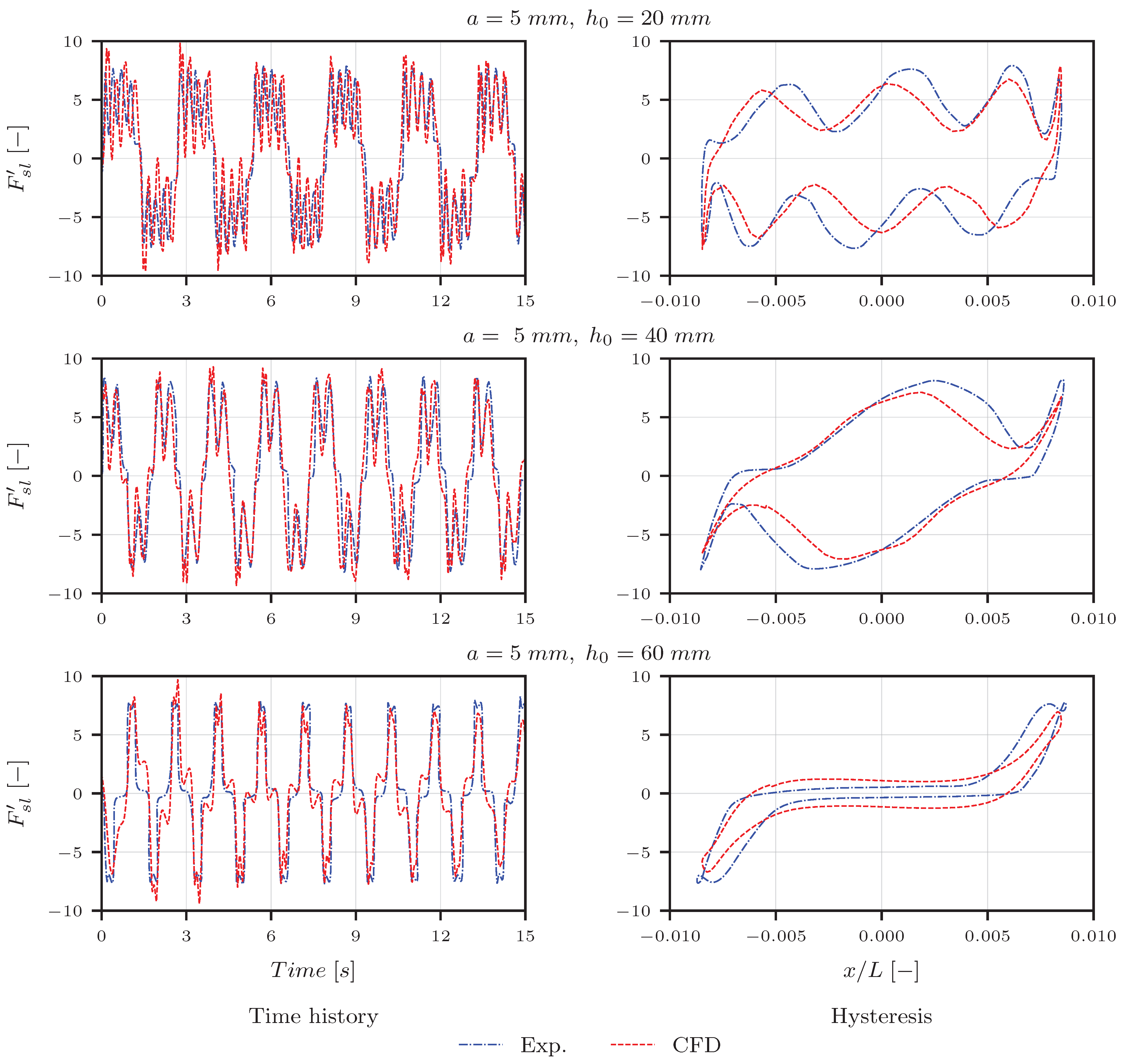
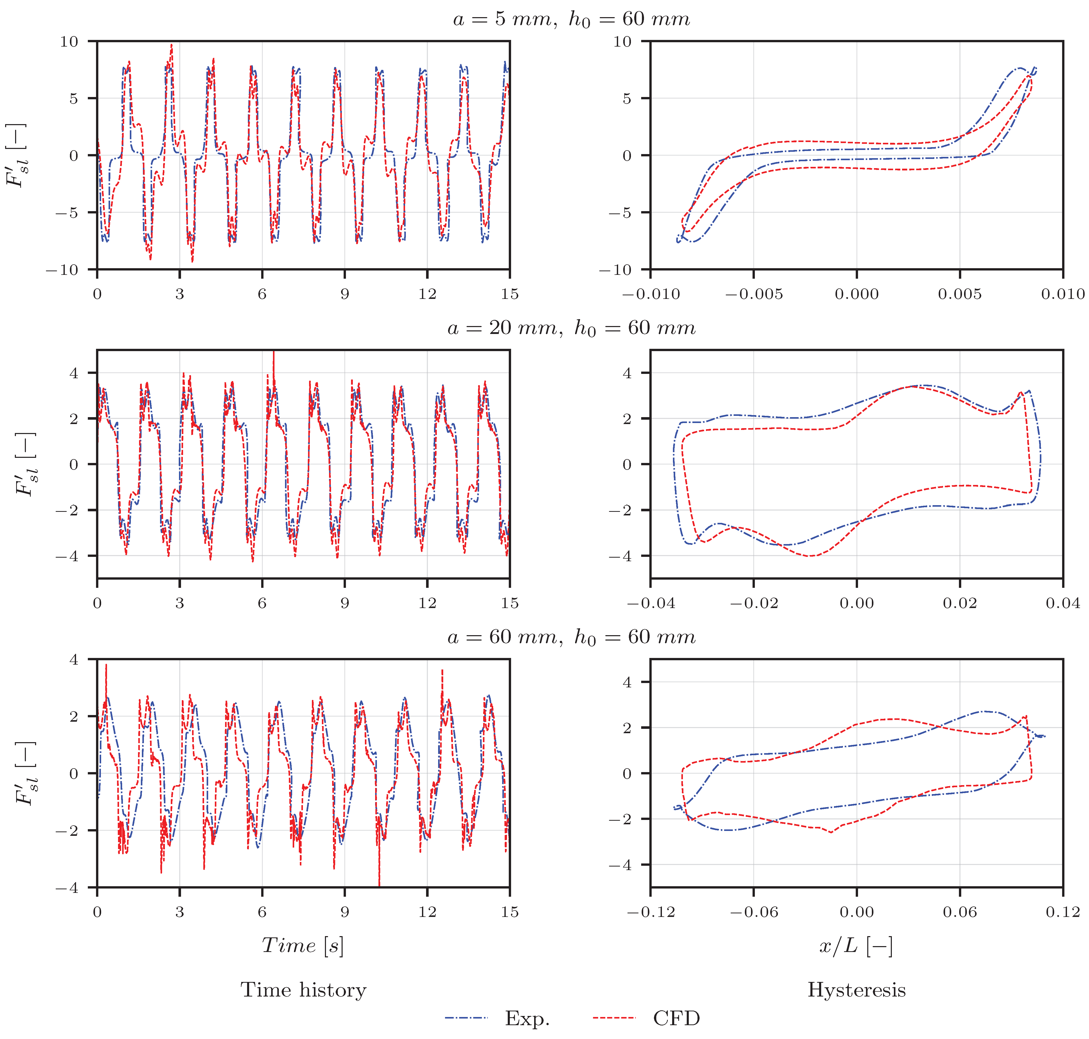
The series of studies was designed using certain parameters from [35], such that the outcome supports the application case of a TSD, as described in [36,37]. We present the sloshing response in the form of the horizontal sloshing force, the shape of the hysteresis curve and the dissipated energy. These values are compared to the reference results in [35]. The comparison is supported by using the dimensionless expressions in Equations (8) and (10). The effect per vibration cycle is of focus, where the enclosed area in the hysteresis loop represents the dissipated energy. We calculated the relative deviation of the assessed values from the results in [35].
Whereas the detailed results are contained in [21], here, we particularly focused on representing the characteristic outcome relevant for further design steps. The deviations observed in Figure 3 and Figure 4 are low. Accompanying quantitative results are presented in Table 1. Not only are the areas of the hysteresis loops very close, but also the shape of the curves depict a comparable behaviour. For cases with a high water depth and small amplitude ratios, the simulations tend to slightly overestimate the sloshing response. We attribute this to additional internal numerical damping for such cases. Overall, the CFD-based approach reproduces the nonlinear sloshing forces very reliably. It can be seen that even higher harmonics are captured by the model, despite the hysteresis loops not identically overlapping with the reference ones.
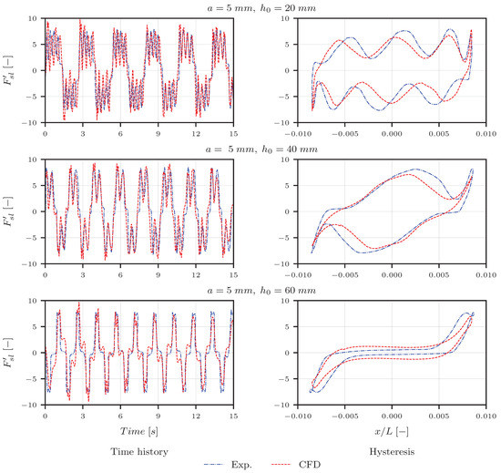
Figure 3.
Validation results for varying the water height.
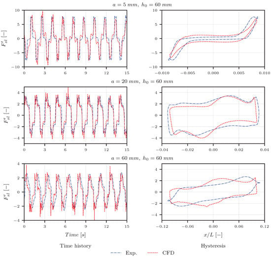
Figure 4.
Validation results for varying the amplitude of excitation.

Table 1.
Dimensionless energy per hysteresis cycle.
Such studies can be designed in various ways, depending on the exact aim. For our use case, we limited them to a two-dimensional domain, without extensive focus on varying the excitation frequency. The results are mainly related to the effect of varying depth and amplitude ratios at a frequency characteristic for our building. It is expected of the TSD to have to mitigate motions that are unidirectional, so this assumption is deemed appropriate. For other cases, three-dimensional simulations might be the only viable alternative, which is possible with CFD simulations.
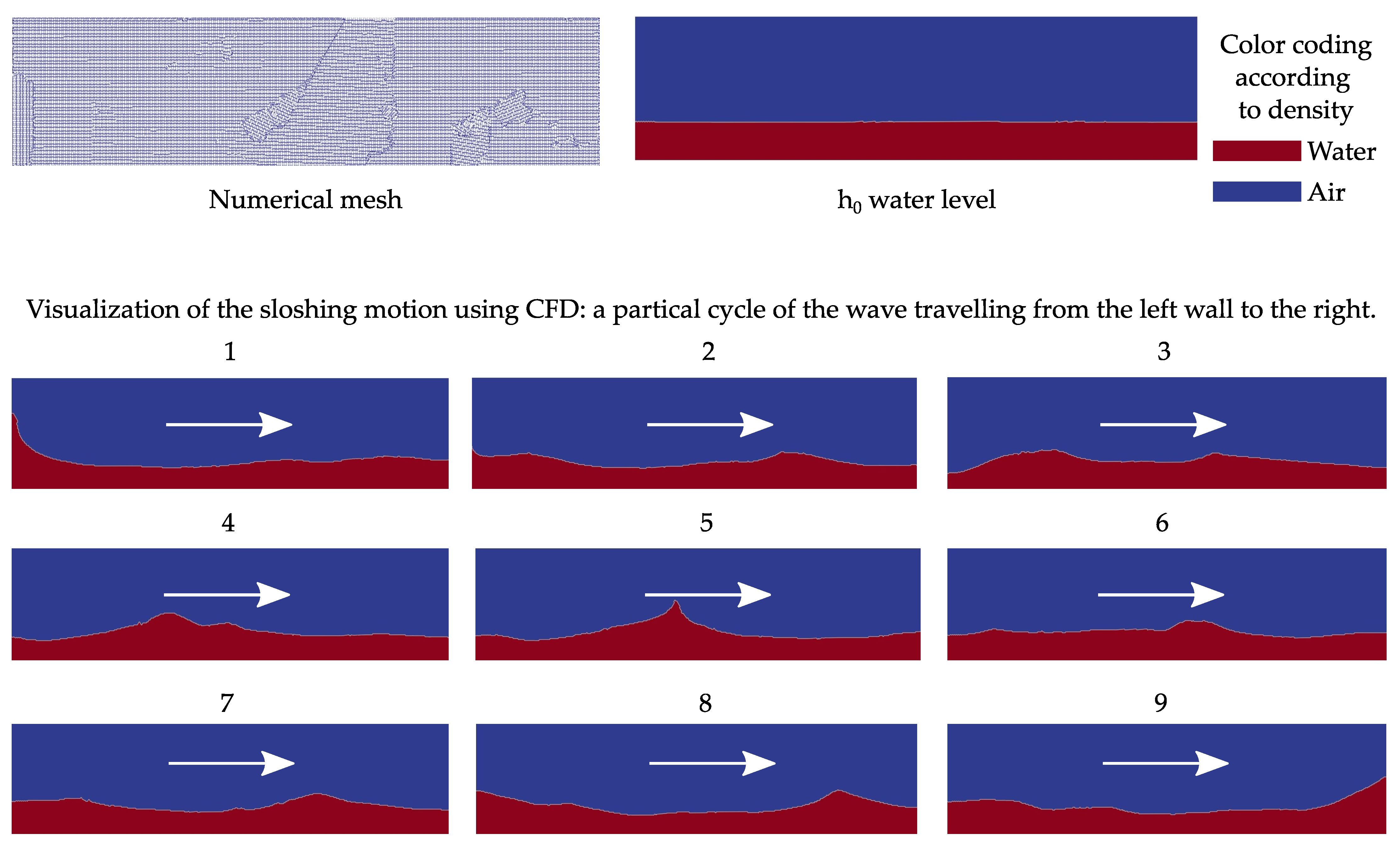
Computational methods make it possible to visualize various results. In Figure 5, we include one of these, as a selection of variables and properties can be captured. Here, we see the clear distinction between air and water based upon density (similarly possible based upon viscosity). Additionally, the velocity and pressure fields are also available to aid in various discussions and design purposes.
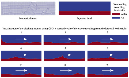
Figure 5.
Showcasing the representative setup and qualitative results for the imposed motion of mm and mm: the water surface being best identified by the border between the densities of air and water.
4. Wind Loading and Vibration Mitigation
Wind loading represents a characteristic load case for tall buildings. It is critical to ensure structural safety and occupational comfort during the design process. Due to the inherent slenderness, high-rises are prone to vibrations. This leads to the necessity to find ways to mitigate such oscillations. Added devices constitute a common way to counteract these effects, with them being either planned already in early design phases or sometimes even considered as part of retrofitting measures. In particular, passive AMDs represent a common solution to wind-induced vibrations. We choose the prototypical case of a sharp-cornered construction, the CAARC-B building. The advantage of this example is that the load conditions are thoroughly studied. Multiple references substantiate the knowledge base, as it represents a benchmark for building aerodynamics. Not only is the oncoming naturally turbulent wind described in detail, but also vortex-shedding characteristics are well-known. This cuboid shape is prone to such a phenomenon, typically resulting in a von Kármán vortex street [38]. Clear vortical structures (more dominant in the case of low-to-no incoming turbulence) are linked to nearly harmonic cross-wind excitation forces.
4.1. Structural Model
The benchmark building has the aspect ratio of its dimensions height H: depth D: width W of 6:1.5:1, with m. With a prescribed density of , the total mass results in . It is a generic structure, with the mass, stiffness and damping characteristics distributed homogeneously. Further provisions give the target modes of vibrations and respective frequencies. The first three for such a cantilever structure are as follows: weak bending at , strong bending at and torsion at . These eigenmodes are uncoupled.
The initial study aimed to use this model for base-force measurements according to the High-Frequency Force Balance (HFFB) method. The peculiarity for that method is that the fixity is flexible, but the building is rigid along its height. As a result, the mode shapes are linear. We created a model setup for Finite Element Analysis (FEA). This numerical replica was built up with elements using a formulation corresponding to the FEM. It led to a structure detailed with multiple types of elements, such as shells, trusses and beams, tuned to match the prescribed geometric and mechanical properties. This directly led to more realistic shapes of vibration, similar to those known for cantilever-type structures.
4.2. Considered Load Cases
Wind loading is numerically captured using a LES approach, typical in CFD for transient flow fields [39,40]. The respective numerical domain follows the setup as presented in [41]. There are certain particularities to this setup, depending on whether the aim is to realistically model the natural turbulence in the Atmospheric Boundary Layer (ABL) or whether the scope is to trigger strong vortex shedding. The former case implies nonzero turbulence, whereas the latter can become critical for very low (to practically zero) turbulence intensity. In Figure 6, we show the main aerodynamic considerations and definitions.

Figure 6.
Definition of the wind loading: direction and simulation domain.
4.2.1. Turbulent Wind Loading
Here, we focus on the excitation typically arising in the Atmospheric Boundary Layer (ABL). Fluctuations in the wind field occur naturally for the CAARC-B, with available provisions describing the target state. This is characterized by the (streamwise, time-averaged) mean velocity profile along the height, accompanied by the turbulence intensity, as well as the (integral) turbulence length scale for this velocity component at the top of the structure. To achieve this state, we numerical modeled the inlet by synthetic turbulence, a specific type of generated condition (using the WindGen generator [42] based on the theory by [43]). We provide our assessment, additionally including the Power Spectral Density (PSD) for the streamwise velocity component. As the velocity is directly linked to the surface pressure, the along-wind excitation force will have a similar spectrum. This scenario is thus characterized by a broad-band excitation, mostly in a streamwise (i.e., along-wind) direction.
The load mechanism is typically dominated by the oncoming flow, this being the gustiness approaching the ABL. It is acceptable to assume that the deformation state of the structure will not have a strong influence on the flow field itself. Consequently, we recorded the wind forces by CFD and applied it on the structural model, as typically carried out in Computational Structural Dynamics (CSD). Following the approach defined as One-Way Coupling (OWC), forces are transferred to the structure, but the resulting deformation state is not updated in CFD.
4.2.2. Oscillations in Smooth Flow
Fluctuations in the flow can either exist without the presence of the structure, such as the case in the previous scenario, or additional ones can arise due to a body being immersed into the flow. The CAARC-B is a bluff body that will facilitate vortex creation around it. Of particular interest is the case of a smooth flow, which triggers dominant shedding around the building. The critical situation is when the vortex shedding frequency matches one of the lower eigenmodes of the structure. We planned a setup to trigger this mechanism for the weak bending mode.
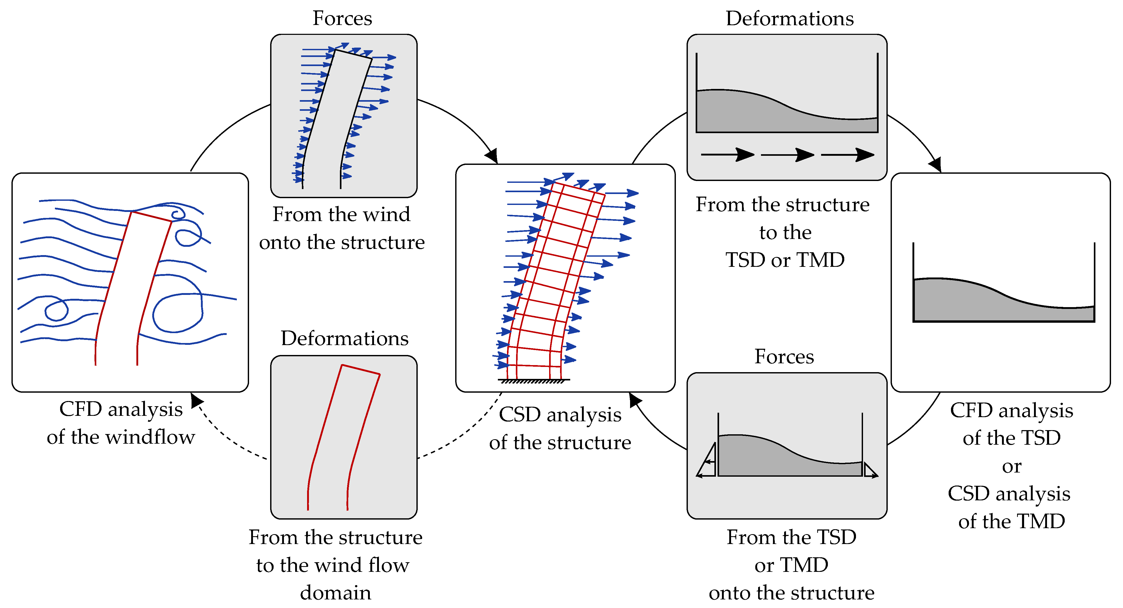
At a particular angle of attack, this occurs for a given streamwise velocity. This is described in detail by [41]. It leads to a practically constant along-wind force accompanied by a close-to-harmonic cross-wind component. If the narrow-banded excitation force [44] exactly matches the underlying structural frequency, we are led to the situation of mechanical resonance. However, in the case of (wind) flow, vortex-shedding can trigger a feedback mechanism, also called lock-in [38]. This means that not only is the exact overlap of the frequencies dangerous, but also the slight shifts might need considering, as the oscillating systems could synchronize. This leads to the necessity of the approach labeled as Two-Way Coupling (TWC). In the numerical context, this means that forces simulated by CFD trigger deformations in the CSD model, which, in turn, will require an update of the shape in the flow field.
4.2.3. Simulated Conditions
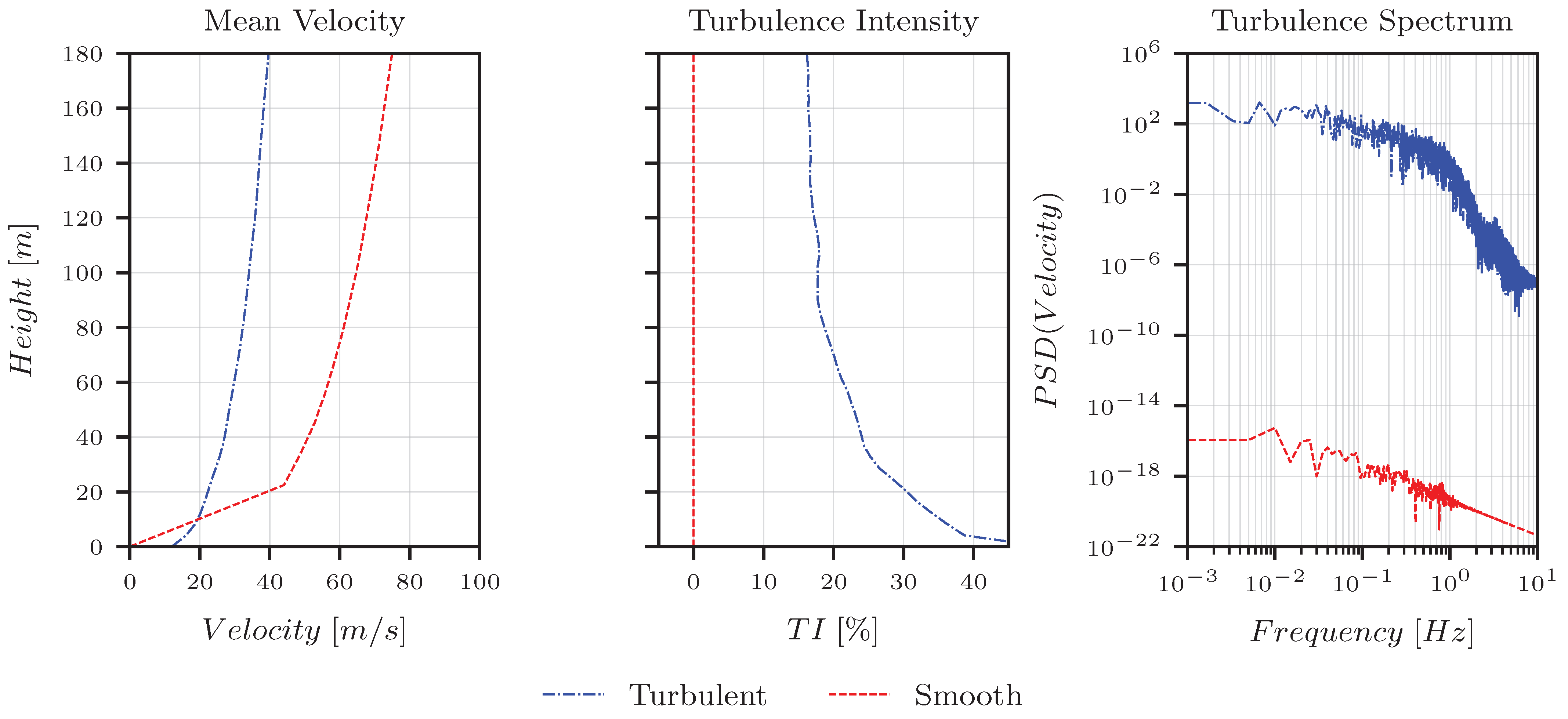
Wind flow conditions are characterized with typical metrics of the streamwise velocity component, presented in Figure 7. The turbulent flow approaches the building at a angle of attack (streamwise perpendicular to the wide face). This is defined by a lower mean magnitude at a higher turbulence intensity . The energy spectrum of this velocity contains higher energy distributed over multiple frequencies. Smooth flow (i.e., minimal to no oncoming fluctuations) is seen in the case of the angle of attack (streamwise parallel to the wide face). For this latter scenario, the along-wind velocity component has lower energy, as observed in the spectrum.
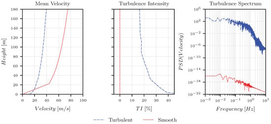
Figure 7.
The typical metrics for characterizing the flow conditions: turbulent for the angle of attack, smooth (i.e., low turbulent) for angle of attack.
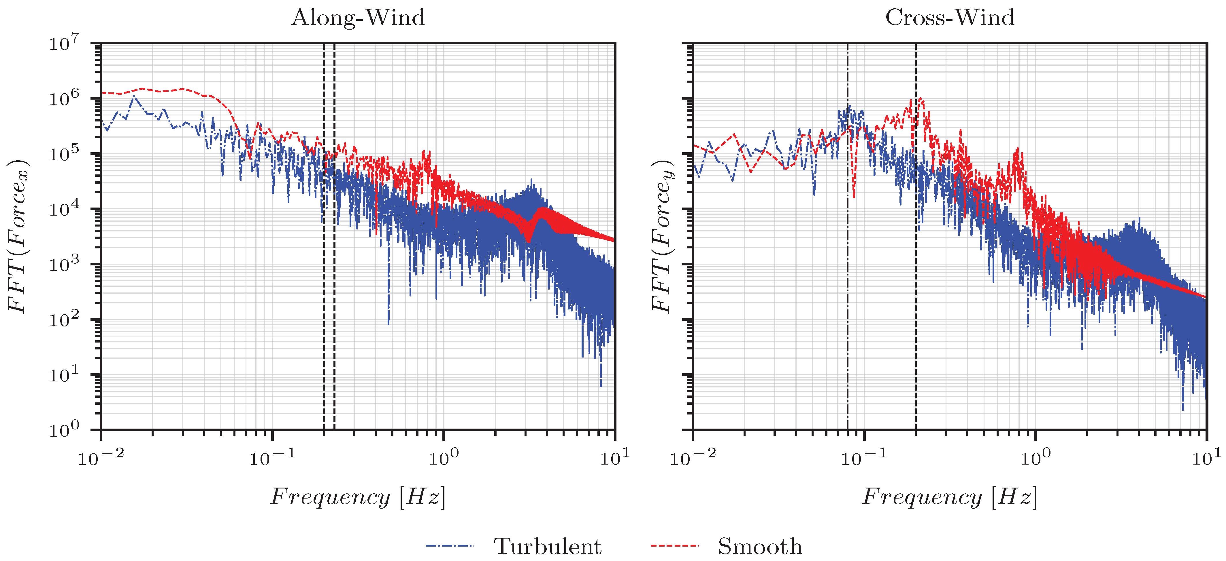
The energy content of the flow is inherent to the natural conditions of the approaching wind. The shape of the building determines the characteristics of the aerodynamic forces that arise under such conditions. These are presented in Figure 8. Along-wind, the vertical lines (dashed) represent the weak and strong bending frequencies, with Hz and Hz. We can see that there is no peak in the energy content at these values. Conversely, for the cross-wind component, the smooth flow peaks at approximately Hz (dashed), with it matching the weak bending mode. In the case of approaching turbulence, we can also observe a cross-wind peak at Hz (marked as dash-dotted). This peak is expected as, also in turbulent conditions, vortex shedding will exhibit itself. However, the mechanism overlaps with the fluctuations already present in the oncoming flow field.
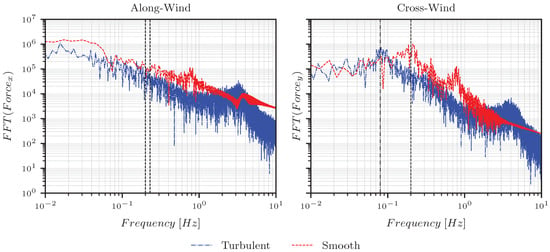
Figure 8.
Spectral assessment of the energy content in the aerodynamic forces: turbulent flow for the angle of attack, smooth in case of angle of attack.
4.3. Coupled Simulations in CWE
Wind effects on structures often imply a feedback mechanism, thus rendering arising phenomena as challenging to be investigated. This means that the force deforms the structure, whereas such changes in shape will alter the flow field, leading to a modification of the excitation itself. This is a crucial characteristic in the case of flexible constructions. Numerical methods constitute one of the viable ways to investigate such effects. The main advantage is that corresponding simulations are not affected by scaling as the digital models are created at full (i.e., real) size. Following a partitioned approach, dedicated solvers are linked to the wind flow and structure, respectively. Nonetheless, this will lead to particular requirements of corresponding computing power, alongside issues related to the accuracy, robustness and stability of the scheme. Additional details characterize the kind of coupling schemes used, OWC or TWC. This choice is problem-dependent, with potential effects being highlighted by the aerodynamic and elastic studies in [45]. Further generalizing the partitioning, numerical simulations permit the inclusion of additional components, such as AMDs, as shown in Figure 9. Whereas extending a structural model with a TMD would be straightforward by adding additional entries in the mass, damping and stiffness matrices (native to the FEM-formulation of structures), this is not a universal solution. For the particular case of a CFD model for a TSD, this submodule (or component) has to be treated in a dedicated manner. It also needs to be included in the broader computational scheme. The generalized concept follows the developments in [41,46]. This is a viable approach for investigating the efficiency of TSDs and TMDs alike, at full scale, while capturing all relevant details. It is also possible to use it for general controllers, with the applicability highlighted by [47].
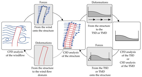
Figure 9.
Representation of the coupled wind–structure–damper simulation.
For our purpose, we set up the TMD and the TSD based on the presented structural properties and following the principles enumerated in Section 2. In Table 2, all crucial parameters are detailed for the weak and strong bending mode, respectively.

Table 2.
Setup of the interacting systems—tructure and AMDs—using the definitions based on the structure-attached coordinate system.
5. Results
This section focuses on presenting the kinematics at the top of the building. We included the time series for the two orthogonal directions, for the displacement as well as the acceleration. These are the typical quantities of interest for the design. Baseline results characterize the motion of the structure under wind loading, without any AMD.
The broad-band excitation is caused by naturally turbulent wind. For this, engineers typically consider a 10-minute time frame, as that is deemed statistically stationary and representative for relevant actions on structures [48]. The initial time phase of s (as seen in Figure 10) represents the initiation phase, with these values being discarded for the quantitative evaluation. Specific metrics are evaluated and shown in Table 3. The along-wind response is comparable, with the TMD and TSD performing similarly, at approximately relative of each other. For the cross-wind direction, the TSD performs at around worse than a TMD under these settings. Both AMDs improve the structural response by mitigating deflections up to . We mention that such devices aim to perform well for excitation forces near the natural vibration of the underlying construction. However, this load case is broad-banded, so less efficiency is to be expected.
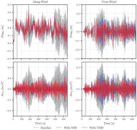
Figure 10.
Time series of the kinematics of the top point under turbulent wind loading.

Table 3.
Statistics of the kinematics of the top point under turbulent wind loading.
Time series are accompanied by a quantitative statistical evaluation. As an additional metric, we define a maximum value based upon derived quantities, instead of the sample maximum. In Equation (11), the estimate is shown using a peak factor (with an estimate provided in this magnitude by [48]) alongside the mean and standard deviation of the time series,
A dedicated discussion on the exact choice of the peak factor is out of the scope of the current study, as it serves here as an amplification factor. It is taken as the same throughout the statistical analysis, with its magnitude deemed representative. For special design cases, this term needs a more in-depth investigation. Table 3 provides a summary. Alongside the absolute values, the relative error is also displayed, being evaluated in pairs, between the TMD–baseline, TSD–baseline and TSD–TMD.
Our second scenario represents narrow-banded loading in the cross-wind direction. The dominant force arises in the smooth flow as a result of vortex shedding. Such an excitation case is more typical for the setting that is aimed to be mitigated by AMDs. Passive devices typically work well at particular frequencies. In Figure 11, we include the times series for displacements and accelerations. This is amended by the statistical evaluation in Table 4. The total time used for the evaluation is s, with the initialization being s. This choice resulted from capturing at least periods of the vortex shedding (with s for the shedding frequency Hz matching the weak bending). We can clearly see in the time series that, for the baseline case, around s are necessary to reach the stationary state of damped harmonic oscillations. To put this in context, these very specific flow conditions for a tall structure would need to be stable for min to arrive at this state, where it would imply m oscillations at a m height. Both AMDs would be able to reduce this to well under m.
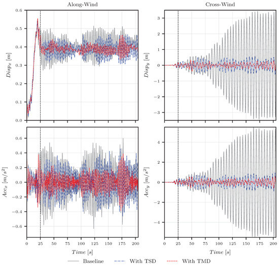
Figure 11.
Time series of the kinematics of the top point in smooth flow.

Table 4.
Statistics of the kinematics of the top point in smooth flow.
A TMD was set up using an assumption of the linear mechanical model particularly tuned to the eigenfrequencies of the building. For TSDs, this is the analogous workflow, yet the tuning process is more complicated. It needs additional considerations of the initial representative response and the amount of mitigation that is aimed to be achieved. Thus, the design is a function of the response amplitude. Altering load conditions would theoretically lead to different optima. We based our considerations on a representative amplitude of acceleration of around (0.15–0.2) m/s for the baseline structure. This value seems to be more appropriate for the broad-band load case, and sub-optimal for the narrow-banded one. A proper decision for each particular design will need to be taken, weighing in the relative importance of specific load cases.
For the particular scenario of smooth flow, both AMDs achieve a considerable improvement of close to 100% cross-wind. In the along-wind direction, the TSD performs clearly worse than the TMD. It needs to be mentioned that, for this load case, the harmonic loading around the weak axis is more critical. Still, the relative performance in this direction shows a considerable difference of 100%, in favor of the TMD.
Accompanying these qualitative and quantitative outcomes on the direct effect of AMDs on structures in wind, we provide a snapshot of representative results. Using computational methods permits analyzing all systems involved at full scale, at various levels of detail. In Figure 12, we include typical data that help to visualize: wind loading using CFD, the structural response captured with CSD and the sloshing motion enabled by CFD. This depiction complements the abstraction of the workflow shown in Figure 9.
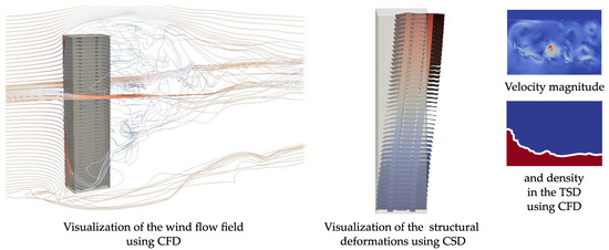
Figure 12.
Representative visual results using a computational workflow.
The complexity of the models and computational effort for the analyses are substantiated by Table 5 and Table 6. Here, we document certain characteristics related to the detailing of the numerical setup. This is best represented by the number nodes and respective variables, the key quantities for a FEM-based formulation. The total duration and amount of time steps will further influence the requirements in the case of transient simulations. The second table includes the approximate computational cost in the form of core hours. We provide it as the magnitude should be meaningful for the engineering practice, as well as to those aiming at similar studies.

Table 5.
Complexity of the numerical models.

Table 6.
Numerical effort required for assessment.
In Table 6, computed core hour values are shown, which we documented for simulations carried out on the same hardware. It can be observed that CFD simulations with turbulent wind will require more capacities because there needs to be a refinement of the mesh from the inlet to the structure to maintain approaching turbulence. Additionally, the total simulation time is typically longer. Despite a larger time step (in this particular case), the resulting effort can be two to three times higher than for the CFD simulation in the case of smooth flow. FSI approaches tend to increase the cost by a factor of at least 2 due to TWC. Including AMDs into the workflow further magnifies requirements by at least a factor of (1.5–2).
6. Conclusions and Outlook
Our work focused on modeling and numerically simulating the effect of added damping systems on structures excited by wind. In particular, we contributed a fully computational workflow that uses CFD not only to capture wind flow but also to include TSDs. This happens in a coupled manner to enable interaction at full scale. Consequently, such an approach currently represents the highest fidelity method for these kinds of assessments. Further innovation lies in developing proper algorithms, with an implementation supporting modularity and scaling on dedicated computing units. Our results support the argument for applicability in the case of similar user scenarios.
We investigated the vibration mitigation efficiency of TSDs using a two-fluid CFD approach. The results show that these can be considerably less efficient than TMDs for the load cases covered. The specific metrics are related to the displacement and acceleration at the top of the building, under wind load. In particular, the RMS and estimated maximum values of the time series are of interest. The optimal tuning was oriented towards accelerations. This baseline comparison shows that a simple passive TMD will tend to perform better than the equivalent setup of a TSD. We need to recall the challenging design process for this latter category. As this is mostly based on a linear mechanical model, more effort is needed to improve the process itself. The nonlinear behavior of the TSD should be investigated at full scale, ideally with coupling to the structure being modeled and simulated. Additionally, there is much room for improvement when considering the possibilities of sloping bottoms, rounding corners and including screens. One specific configuration of vertical slat screens that we do consider, and its effect, are included in our results. Further numerical optimization would potentially lead to improvements in the performance of TSDs. Additionally, we explored recent numerical advances in finding an appropriate model for the mechanical effects of the considered AMDs. The sloshing motion is realistically simulated by the two-fluid CFD approach. The validation studies of a rectangular container under prescribed motion are well in-line with the experimental reference. This ensures that the effect of sloshing is correctly captured, as substantiated by the time histories and hysteresis curves. The combination of CFD and numerical optimization is a viable way to investigate the effects of TSDs, as well as to find improved designs.
The chosen load cases relate to two representative scenarios, both describing various facets of wind loading on tall structures. Atmospheric turbulence is modeled by a generated synthetic wind, whereas the other scenario aims to trigger strong vortex shedding. Yet again, CFD-based methods are able to properly model such flow phenomena, which contribute to the realistic loading of constructions. The loading itself is set up based on referenced work. Furthermore, the structure is modeled by a detailed numerical replica, including all structural details and resulting in a particular mass, stiffness and damping distribution in space. It is defined at its full size.
Our numerical workflow and framework permits capturing the interaction between the excitation source and the considered structure, as well as the AMDs. This leads to an integrated process where all effects can be simulated at the proper scale and necessary resolution. The current contribution showcased its usability by including AMDs that were tuned for the two orthogonal directions separately, modeled one-dimensional (for the TMD) and two-dimensional (for the TSD). The total damping effect was yielded from superposing reactions. Future work will focus on validating this assumption using three-dimensional models. This shall also enable their usability in structures with coupled bending and torsion.
Author Contributions
Conceptualization, M.P., K.-U.B. and F.W.; methodology, M.P. and A.R.; software, M.P. and A.R.; validation, A.R. and M.P.; formal analysis, M.P., A.R. and F.W.; investigation, A.R. and M.P.; resources, M.P., K.-U.B. and F.W.; data curation, M.P. and A.R.; writing—original draft preparation, A.R. and M.P.; writing—review and editing, M.P., F.W. and A.R.; visualization, A.R. and M.P.; project administration, M.P., K.-U.B. and F.W. All authors have read and agreed to the published version of the manuscript.
Funding
This research received no external funding.
Institutional Review Board Statement
Not applicable.
Informed Consent Statement
Not applicable.
Data Availability Statement
The data presented in this study are available on request from the corresponding author.
Acknowledgments
The authors gratefully acknowledge the Gauss Centre for Supercomputing e.V. (www.gauss-centre.eu) (accessed on 29 May 2022) for funding this project by providing computing time on the GCS Supercomputer SuperMUC-NG at Leibniz Supercomputing Centre (www.lrz.de) (accessed on 29 May 2022). The authors additionally remark the support of Maurer SE, Maurer Engineering GmbH and Maurer Switzerland GmbH.
Conflicts of Interest
The authors declare no conflict of interest.
References
- Wardlaw, R.L.; Moss, G.F. A Standard Tall Building Model for the Comparison of Simulated Natural Wind in Wind Tunnels. CAARC CC 662m Tech 1970, 25. [Google Scholar]
- Melbourne, W.H. Comparison of measurements on the CAARC standard tall building model in simulated model wind flows. J. Wind Eng. Ind. Aerodyn. 1980, 6, 73–88. [Google Scholar] [CrossRef]
- Benchmark Buildings for an International HFFB Comparison. The Study as Proposed by the International Association for Wind Engineering (IAWE). Available online: https://www.iawe.org/committees/HFBB-spec.pdf (accessed on 29 May 2022).
- Holmes, J.; Tse, K.T. International high-frequency force balance benchmark study. Wind Struct. 2014, 18, 457–471. [Google Scholar] [CrossRef]
- Wang, W.; Kamath, A.; Martin, T.; Pákozdi, C.; Bihs, H. A Comparison of Different Wave Modelling Techniques in an Open-Source Hydrodynamic Framework. J. Mar. Sci. Eng. 2020, 8, 526. [Google Scholar] [CrossRef]
- Li, Z.; Deng, G.; Queutey, P.; Bouscasse, B.; Ducrozet, G.; Gentaz, L.; Le Touzé, D.; Ferrant, P. Comparison of wave modeling methods in CFD solvers for ocean engineering applications. Ocean Eng. 2019, 188, 106237. [Google Scholar] [CrossRef]
- Godderidge, B.; Turnock, S.; Tan, M.; Earl, C. An investigation of multiphase CFD modelling of a lateral sloshing tank. Comput. Fluids 2009, 38, 183–193. [Google Scholar] [CrossRef]
- Hwang, S.Y.; Lee, J.H. The Numerical Investigation of Structural Strength Assessment of LNG CCS by Sloshing Impacts Based on Multiphase Fluid Model. Appl. Sci. 2021, 11, 7414. [Google Scholar] [CrossRef]
- Cotela, J.; Oñate, E.; Rossi, R. Applications of Turbulence Modeling in Civil Engineering; Monograph CIMNE: Barcelona, Spain, 2016; Available online: https://www.scipedia.com/public/Cotela_2016 (accessed on 29 May 2022).
- Heil, M.; Hazel, A.L.; Boyle, J. Solvers for large-displacement fluid–structure interaction problems: Segregated versus monolithic approaches. Comput. Mech. 2008, 43, 91–101. [Google Scholar] [CrossRef]
- Degroote, J.; Haelterman, R.; Annerel, S.; Bruggeman, P.; Vierendeels, J. Performance of partitioned procedures in fluid–structure interaction. Comput. Struct. 2010, 88, 446–457. [Google Scholar] [CrossRef] [Green Version]
- Mok, D.P.; Wall, W.A. Partitioned analysis schemes for the transient interaction of incompressible flows and nonlinear flexible structures. In Trends in Computational Structural Mechanics; CIMNE: Barcelona, Spain, 2001; pp. 688–698. [Google Scholar]
- Dettmer, W.G.; Perić, D. A new staggered scheme for fluid–structure interaction. Int. J. Numer. Methods Eng. 2012, 93, 1–22. [Google Scholar] [CrossRef]
- The Kratos Multiphysics Open-Source Project. Available online: https://github.com/KratosMultiphysics/Kratos (accessed on 29 May 2022).
- Dadvand, P.; Rossi, R.; Gil, M.; Martorell, X.; Cotela, J.; Juanpere, E.; Idelsohn, S.; Oñate, E. Migration of a generic multi-physics framework to HPC environments. Comput. Fluids 2013, 80, 301–309. [Google Scholar] [CrossRef] [Green Version]
- Lamb, H. Hydrodynamics; University Press: Cambridge, MA, USA, 1924. [Google Scholar]
- Graham, E.; Rodriguez, A. The Characteristics of Fuel Motion Which Affect Airplane Dynamics. J. Appl. Mech. 1952, 19, 381–388. [Google Scholar] [CrossRef]
- Masó, M.; de Pouplana, I.; Oñate, E. A FIC-FEM procedure for the shallow water equations over partially wet domains. Comput. Methods Appl. Mech. Eng. 2022, 389, 114362. [Google Scholar] [CrossRef]
- Cremonesi, M.; Franci, A.; Idelsohn, S.; Oñate, E. A State of the Art Review of the Particle Finite Element Method (PFEM). Arch. Comput. Methods Eng. 2020, 27, 1709–1735. [Google Scholar] [CrossRef]
- Iaconeta, I.; Oñate, E.; Larese, A. Discrete-Continuum Hybrid Modelling of Flowing and Static Regimes; Monograph CIMNE: Barcelona, Spain, 2019; Available online: https://www.scipedia.com/public/Iaconeta_et_al_2020a (accessed on 29 May 2022).
- Riedl, A.M. Numerical Modeling and Simulation of Coupled TLD-Structure Response under Time History Loading. Master’s Thesis, Technical University of Munich, Munich, Germany, 2021. [Google Scholar]
- Ferziger, J.; Peric, M.; Street, R. Numerische Strömungsmechanik; Springer Vieweg: Berlin, Germany, 2020. [Google Scholar]
- von Wenczowski, S. Two-Fluid Finite Element Formulation for Flood Simulation in Mountain Terrain. Master’s Thesis, Technical University of Munich, Munich, Germany, 2019. [Google Scholar]
- Love, J.; Tait, M.; Toopchi-Nezhad, H. A hybrid structural control system using a tuned liquid damper to reduce the wind induced motion of a base isolated structure. Eng. Struct. 2011, 33, 738–746. [Google Scholar] [CrossRef]
- Tait, M. Modelling and preliminary design of a structure-TLD system. Eng. Struct. 2008, 30, 2644–2655. [Google Scholar] [CrossRef]
- Petersen, C.; Werkle, H. Dynamik der Baukonstruktionen; Springer Vieweg: Wiesbaden, Germany, 2017. [Google Scholar] [CrossRef]
- Hamelin, J. The Effect of Screen Geometry on the Performance of a Tuned Liquid Damper. Master’s Thesis, McMaster University, Hamilton, ON, Canada, 2007. [Google Scholar]
- Cassolato, R. The Performance of a Tuned Liquid Damper Equipped with Inclined and Oscillating Damping Screens. Master’s Thesis, McMaster University, Hamilton, ON, Canada, 2007. [Google Scholar]
- Tait, M. The Performance of 1-D and 2-D Tuned Liquid Dampers. Ph.D. Thesis, University of Western Ontario, London, ON, Canada, 2004. [Google Scholar]
- Tait, M.; Isyumov, N.; El Damatty, A. Effectiveness of a 2D TLD and its numerical modeling. J. Struct. Eng. 2007, 133, 251–263. [Google Scholar] [CrossRef]
- Tait, M.; El Damatty, A.; Isyumov, N. An investigation of tuned liquid dampers equipped with damping screens under 2D excitation. Earthq. Eng. Struct. Dyn. 2005, 34, 719–735. [Google Scholar] [CrossRef]
- Baines, W.; Peterson, E. An investigation of flow through screens. Trans. Am. Soc. Mech. Eng. 1951, 73. [Google Scholar]
- Weisbach, J. Die Experimental-Hydraulik; JG Engelhardt: Freiberg, Germany, 1855. [Google Scholar]
- Gardarsson, S.; Yeh, H.; Reed, D. Behavior of sloped-bottom tuned liquid dampers. J. Eng. Mech. 2001, 127, 266–271. [Google Scholar] [CrossRef]
- Krabbenhøft, J. Shallow Water Tuned Liquid Dampers. Ph.D. Thesis, Department of Civil Engineering, Technical University of Denmark, Lyngby, Denmark, 2011. Available online: https://backend.orbit.dtu.dk/ws/portalfiles/portal/6470255/PhD_Thesis_Krabbenhoft2010.pdf (accessed on 29 May 2022).
- Sun, L.; Fujino, Y.; Pacheco, B.; Isobe, M. Nonlinear Waves and Dynamic Pressures in Rectangular Tuned Liquid Damper (TLD) Simulation and Experimental Verification. Doboku Gakkai Ronbunshu 1989, 1989, 81–92. [Google Scholar] [CrossRef] [Green Version]
- Sun, L.; Fujino, Y. A semi-analytical model for tuned liquid damper (TLD) with wave breaking. J. Fluids Struct. 1994, 8, 471–488. [Google Scholar] [CrossRef]
- Hucho, W.H. Aerodynamik der Stumpfen Körper, 2nd ed.; Vieweg+Teubner: Wiesbaden, Germany, 2011. [Google Scholar]
- Bitsuamlak, G.; Simiu, E. CFD’s potential applications: A wind engineering perspective. In Proceedings of the The Fifth International Symposium on Computational Wind Engineering (CWE2010), Chapel Hill, NC, USA, 23–27 May 2010. [Google Scholar]
- Blocken, B. 50 years of Computational Wind Engineering: Past, present and future. J. Wind Eng. Ind. Aerodyn. 2014, 129, 69–102. [Google Scholar] [CrossRef]
- Péntek, M.; Winterstein, A.; Vogl, M.; Kupás, P.; Bletzinger, K.U.; Wüchner, R. A multiply-partitioned methodology for fully-coupled computational wind-structure interaction simulation considering the inclusion of arbitrary added mass dampers. J. Wind Eng. Ind. Aerodyn. 2018, 177, 117–135. [Google Scholar] [CrossRef]
- Andre, M. WindGen: A Synthetic Wind Simulation Library. Available online: https://github.com/msandre/WindGen (accessed on 29 May 2022).
- Mann, J. Wind field simulation. Probabilistic Eng. Mech. 1998, 13, 269–282. [Google Scholar] [CrossRef]
- Holmes, J. Wind Loading of Structures, 3rd ed.; CRC Press: Boca Raton, FL, USA, 2015. [Google Scholar]
- Andre, M.; Péntek, M.; Bletzinger, K.U.; Wüchner, R. Aeroelastic simulation of the wind-excited torsional vibration of a parabolic trough solar collector. J. Wind Eng. Ind. Aerodyn. 2017, 165, 67–78. [Google Scholar] [CrossRef]
- Uekermann, B.; Gatzhammer, B.; Mehl, M. Coupling algorithms for partitioned multi-physics simulations. In Informatik 2014; Plödereder, E., Grunske, L., Schneider, E., Ull, D., Eds.; Gesellschaft für Informatik e.V.: Bonn, Germany, 2014; pp. 113–124. [Google Scholar]
- Winterstein, A. Modeling and Simulation of Wind-Structure Interaction of Slender Civil Engineering Structures Including Vibration Mitigation Systems. Ph.D. Thesis, Technical University of Munich, Munich, Germany, 2020. Available online: https://mediatum.ub.tum.de/1542819 (accessed on 29 May 2022).
- Tamura, Y.; Kareem, A. Advanced Structural Wind Engineering; Springer: Tokyo, Japan, 2013. [Google Scholar] [CrossRef]
Publisher’s Note: MDPI stays neutral with regard to jurisdictional claims in published maps and institutional affiliations. |
© 2022 by the authors. Licensee MDPI, Basel, Switzerland. This article is an open access article distributed under the terms and conditions of the Creative Commons Attribution (CC BY) license (https://creativecommons.org/licenses/by/4.0/).


