Development of a Multi-Sensor Concept for Real-Time Temperature Measurement at the Cutting Insert of a Single-Lip Deep Hole Drilling Tool

Abstract

The mechanical energy resulting from cutting processes is turned almost completely in thermal energy, which encourages thermal procedures, such as diffusion, leading to higher wear in the cutting tool and thus to higher temperatures. Furthermore, high temperatures influence the properties of the marginal zones in the workpiece. In this presented work, the in-process temperature of a cutting insert during single-lip deep hole drilling (SLD) is investigated. Therefore, a sensor-integrated tool with resistance temperature detectors (RTD) placed beneath the cutting insert is developed. First, the thermal properties of the cutting insert are adjusted to fit the assembled tool. Afterwards, a CEL-Simulation is obtained to examine the temperature distribution at the cutting edge of the SLD-tool. The temperatures calculated by simulation can be compared to the in-process temperatures of the sensor integrated tool. Because of the usage of a cooling lubricant, simulated temperatures can be varied with a factor to fit the experimentally measured temperature curves. The highest temperature during the process appears at the outer edge of the cutting insert. By knowing the thermal properties, the maximum process temperatures for the deep hole drilling operation are to be calculated. The results represent a contribution to an interdisciplinary research project “Surface Conditioning in Machining Processes” (SPP 2086) of the German Research Foundation (DFG).

1. Introduction

Drilling is one of the most used processes in cutting technology, whereas using twist drills is the most common drilling method. Despite the advantages of twist drilling tools, such as low-cost and self centering, some applications have extra requirements with respect to surface quality or length-to-diameter ratio of the bore holes. Deep hole drilling is a drilling process, allowing boreholes with large l/D ratios and a particularly high surface quality. The production of deep bore holes via single-lip deep hole drilling tools utilizes asymmetrical single-edged tool designs. The asymmetrical single-edged drilling tool requires special guidance because of a resultant force coming from the process cutting forces. The guidance outside of the workpiece consists of a drill bush and, depending on the tool length, additional steady state rests. While drilling, the guide pads of the tool, which have a slightly larger effective diameter than the cutting edge, plastifies the wall of the bore hole. That interaction leads to high surface qualities and compressive residual stresses in the subsurface through forming interactions between the tool and workpiece [1,2]. The main problem producing deep bore holes is a reliable chip removal. Therefore, a cooling lubricant is fed under high pressure through the shaft of the drilling tool. The aim of the cooling lubricant is, on the one hand, cooling down the process and, on the other hand, the chip removal from the chip formation zone. High process temperatures can also affect the marginal zones of the bore hole wall [3]. Oezkaya also simulates the chip removal process from the effective area of the cutting edge of a SLD tool. No sufficient cooling lubricant can be found at the outer edge of the cutting edge [4].

The temperature in the cutting zones has a significant influence on the deep hole drilling process [5]. In order to determine the temperature directly at the cutting edge, a concept was developed in this work that can be used to derive determination equations from experimental temperature measurement data and simulation results that predict the temperature directly in the cutting zone. These equations can be used for real-time control in the future. Among other things, a sensory tool was used for the temperature measurements, with three PTC sensors integrated here under the cutting insert [6]. In order to investigate the temperature in a two-dimensional state, orthogonal cuts were performed presenting experimental and simulational chip formation, frictional impacts and the resulting temperatures [7,8]. To study the SLD process, several investigations were carried out. Via Lagrangian simulation, thermographic camera and PTC resistance sensors, the thermal as-is state was examined [9,10]. In addition, the influence of the thermomechanical condition on the subsurface during deep drilling was considered. A thermocouple was used to determine the temperatures on the workpiece side at various process parameters. Coupled Eulerian–Lagrangian (CEL) simulations were carried out to compare the feed forces and the residual stress state in the subsurface [11]. Further investigations studying the thermomechanical impact of SLD on the surface integrity concentrates in temperature measurements with thermocouples and a pyrometer and various cooling lubricant strategies [12,13]. Based on this, a temperature determination of the tool cutting edge during the deep drilling process is to be made possible.

2. Materials and Methods

2.1. Determination of Thermal Properties

The main problem determining the in-process temperature in drilling tools is the inaccessibility of the impact zone of the tool. That is why only indirect temperature measurements are possible. The used tool is a SLD tool with a diameter of D = 18 mm and a length of l = 700 mm with a cutting insert and screwed guiding pads. The temperature propagation in the cutting insert is to be measured. Figure 1 shows the drill head with the PT1000 resistance sensors S1 to S3, placed beneath the cutting insert of the SLD tool. A load-free installation of the sensors is a condition for obtaining proper temperature values. Pressure applied to the sensors during cutting process leads to a deviation of the measured values. PT1000 sensors have the advantage of a fast response characteristic and small installation space specifications. The circuit board equipped with the sensors was placed in a slightly deeper pocket under the cutting edge. The sensors were then completely covered with 2C epoxy resin and cured. This setup avoids pressure-related measurement inaccuracies and isolates the electric measuring equipment from the cooling lubricant. A Seria rotarX slip ring from B-COMMAND GmbH (Hamburg, Germany) was used for data transmission. The cables passing through the cooling channel are connected to the slip ring and thus led the sensor data to the measuring computer.

Embedding the temperature sensors and assembling the cutting insert changes the heat transfer characteristics from the cutting edge to the sensors. With a heat transfer simulation, the thermal quantities of conduction, specific heat and the heat transfer coefficient due to convection were adjusted in a preliminary test. In this way, the heat transfer properties of the tool were identified in order to enable a recalculation of the applied temperature at the cutting edge. The cutting insert was implemented in the heat transfer simulation and discretized with 4-node linear heat transfer tetrahedral (DC3D4) elements. For the reverse engineering experiment, the air mass flow of a hot air soldering gun was set to a volumetric flow rate of $\dot{V}$ = 60 L/min. The temperature of the soldering gun $T_{\mathrm{heat}}$ = 300 °C was checked with the test of a 935 temperature measuring device at a working distance of 2 mm. The air flow was then directed at the same working distance to the outer surface of the cutting edge. For the heat transfer simulation representing the preliminary test, a defined convection was applied to the cutting insert. A temperature of $T_{\mathrm{airflow}}$ = 200 °C was measured with the thermocouple at the working distance. Thus, the heat transfer coefficient due to free convection $\alpha$ can be determined approximately via the analytical equation.

$$v=\frac{\dot{V}}{A}=\frac{\dot{V}}{\pi ·r^2}=141.5\frac{\mathrm{m}}{\mathrm{s}},$$

(1)

$$\alpha =12·\sqrt{v}+2=144.75\frac{\mathrm{W}}{{\mathrm{m}}^2\mathrm{K}},$$

(2)

In addition, the surface area at which the airflow is impinging the cutting edge was determined via the shear layer, which is caused by the expansion of the airflow after exiting the nozzle. Via a defined heat flow onto the calculated surface, the cutting insert is heated according to Figure 2. With a diffusion angle of $\Theta$ = 10°, at which the air flow velocity attenuates to 1%, the working distance of 2 mm and a nozzle diameter of 2.6 mm the impact area results in a radius of 1.617 mm with T_airflow. A heat radiation from the cutting insert was applied to the free surfaces with a factor of 0.9.

The heat transfer simulation uses the material parameters of tungsten carbide with a carbide content of 15%. The set material parameters can be taken from

Table 1. Material parameters of tungsten carbide adapted from [10].

Density $\mathit{\rho }$/ kg/m${}^3$	Young’s Modulus E/ MPa	Poissonsratio $\mathsf{\mu }$/ -	Thermal Expansion $\mathit{\xi }$/ $\mathsf{\mu }$m/mK	Conductivity k/ W/mK	Specific Heat ${\mathit{c}}_{\mathit{p}}$/ J/kgK
15,700	524,000	0.23	6.3	82.24	579.45

.

With these parameters, first a heating simulation is performed. In the simulation, the tool is heated to a certain temperature level coming from the experimental results of the heat transfer. The thermal state of the tool is used to transfer the temperatures at the node points to a subsequent cooling simulation, where the tool is cooled down to room temperature in a certain time.

2.2. CEL Simulation of the SLD Process

For the simulation of the drilling process, the CEL method was used to calculate the problem. This simulation method has already been successfully used for machining simulations [8,11], mostly an orthogonal cutting process, and offers many advantages compared to an explicit Lagrangian simulation when dealing with problems with large deformations. The material 42CrMo4+QT (AISI 4140) was used for the investigations. This is a quenched and tempered alloyed stainless steel with high strength and high toughness. The material is mostly used for highly stressed components with high toughness requirements. The temperature-dependent thermal properties describing the workpiece material behavior at different temperatures are listed in

Table 2. Material parameters of 42CrMo4 adapted from [10].

Young’s Modulus E/ MPa	Thermal Expansion $\mathit{\xi }$/ $\mathsf{\mu }$m/mK	Conductivity k/ W/mK	Specific Heat ${\mathit{c}}_{\mathit{e}}$/ J/kgK	Temperature T/ K
217,000	10.8	-	291.24	173
213,000	11.7	-	354.03	273
212,000	11.9	41.7	361.89	293
207,000	12.5	43.4	389.36	373
199,000	13.0	43.2	418.41	473
192,000	13.6	41.4	445.88	573
184,000	14.1	39.1	479.64	673
175,000	14.5	36.7	531.45	773
164,000	14.9	34.1	610.73	873
69,000	14.9	34.1	610.73	1773

. These are of particular importance in deep drilling processes since the heat in a borehole propagates into the material in all directions. The inelastic heat fraction can be used in thermomechanical problems to determine which fraction of the inelastic energy is converted into heat. By default, a value of 0.9 is assumed.

For the plastic material behavior, the so called Johnson–Cook (JC) model was used, which is widely applied for machining simulations. With the parameters A, B, C, m, n and the material parameter ${\dot{ϵ}}_0$ for the strain rate and the room temperature, as well as the melting temperature, the following equation is obtained:

$$\sigma =[A+B·{ϵ}^n][1+C·\frac{\dot{ϵ}}{{\dot{ϵ}}_0}][1-{\left(\frac{T-T_{room}}{T_{melt}-T_{room}}\right)}^m],$$

(3)

The values for the calculation of the plastic material behavior are presented in

Table 3. Johnson–Cook parameters of 42CrMo4 adapted from [10].

A/MPa	B/MPa	C/ -	n/-	m/-	T${}_{\mathit{melt}}$/K	T${}_{\mathit{room}}$/K
595	580	0.023	0.133	1.03	1793	300

.

To consider the damage of the material, the JC damage model was implemented, which can be described with the values in

Table 4. Johnson–Cook damage parameters of 42CrMo4 adapted from [10].

${\mathit{d}}_1$/-	${\mathit{d}}_2$/-	${\mathit{d}}_3$/-	${\mathit{d}}_4$/-	${\mathit{d}}_5$/-	${\mathit{T}}_{\mathit{melt}}$/K	${\mathit{T}}_{\mathit{transition}}$/K	${\dot{\mathit{ϵ}}}_0$/1/s
011	0.04	−0.02	1	0.12	1793	300	1

.

For an optimization of the large computation times for three-dimensional problems, the density of the materials was increased by a manual mass scaling (MS) to such an extent that an acceptable stable time increment results. The maximum time increment $dt$ depends on the characteristic element length L and the acoustic wave speed $c_d$. Here the density $\delta$ occurs in the denominator and provides a small propagation velocity, which results in larger time increments [14]

$$dt=\frac{L}{c_d};c_d=\sqrt{\frac{E}{\rho }};\rho =\frac{m}{V},$$

(4)

Due to the relation of the density with the specific heat capacity, even the specific heat capacity has to be adjusted. With the CEL approach, increasing the density changes the right-hand term of equation:

$$k{\nabla }^{2}T=\xi \lambda T_{0}tr\left(\dot{E}\right)+\rho c_p\dot{T},$$

(5)

the thermal time constant. Here, $\lambda$ and $\mu$ represent the Lamé coefficients, and $T_0$ the reference temperature. This effect can be compensated if the specific heat capacity $c_p$ is reduced by the same factor that the density $\rho$ is increased with. The mechanical behavior of the system can be described with Navier’s equation for thermoelasticity with the displacement vector u:

$$\mu {\nabla }^{2}u+(\lambda +\mu )\nabla tr\left(E\right)-\xi \lambda \nabla T=\rho \frac{\partial u}{\partial t^2}.$$

(6)

Since the right-hand side of the equation is increased as the density is increased, there is also an increase in the maximum stable time increment [15].

During machining, forces and temperatures are strongly influenced by friction, which requires an accurate friction modeling. Different modeling approaches are distinguished. The used Coulomb friction can be implemented as a constant value in the simulation. The set friction values between tool and workpiece are decisive for the resulting process temperatures. With a Coulomb friction value of $\mu$ = 0.6, which can be taken from the data sheet for the coating of the cutting insert (FIRE coating, Gühring KG), a process heat transfers a certain amount of the kinetic energy into heat, which is distributed in different fractions to the workpiece and the tool. To build up a CEL simulation in Abaqus 2020, Dassault Systémes SE (Vélizy-Villacoublay, France), three bodies are needed. These different bodies are shown in Figure 3. The Eulerian section, representing the entire region of the cutting process where material can be found, uses 8-node thermally coupled linear Eulerian brick elements (EC3D8RT). This material is calculated by a volume fraction of a Lagrangian body placed inside the Euler body, that should not be discretized. Thus, a material filling state is specified in all elements of the Euler body. In addition, the tool is transferred to the simulation as deformable part with a rigid constraint. The discretization of the tool with 4-node thermally coupled tetrahedral, linear displacement and temperature dependent (C3D4T) elements was applied. The material was assigned to each of these bodies via a section. The material models described above were applied for this purpose. In addition, the ambient temperatures were defined and the movements of the tool were set via boundary conditions. Here, the feed motion was executed via the Euler body. On the bottom of the Euler body, the material filling is automatically updated, which allows the workpiece to be machined at very shallow depths. The tool executes the rotary movement of the drill via a reference point. The remaining degrees of freedom are fixed. The advantage of the CEL simulation is the realistic representation of feed and cutting speed with simultaneously acceptable calculation times. Thus, the cutting speed is first set to $v_c$ = 80 m/min and the feed rate f = 0.05 mm/rev. These represent standard process parameters in deep hole drilling processes of 42CrMo4 [2]. The main goal of the simulation is to obtain the temperature distribution at the cutting edge for a stable process point.

2.3. Experimental Study

For the experimental investigation of the temperature during the drilling process, a two-level full factorial experimental design was created with the software Minitab^®19.2020.1, Minitab, LLC (State College, PA, USA) using an effective area model with the recommended default settings. The selection of the process parameters was based on the standard VDI 3208 for deep drilling with SLD under variation of the cutting speed $v_c$ and the feed f [2]. For interpretation, the results can be plotted at the star points in three dimensions in an effective area plot. The process parameters of the experimental design are shown in

Table 5. Experimental design.

Nr.	Cutting Speed ${\mathit{v}}_{\mathit{c}}$/m/min	Feed f/mm/rev
1	59.82	0.02750
2	77.50	0.02750
3	90.00	0.04500
4	77.50	0.00275
5	95.18	0.02750
6	65.00	0.01000
7	65.00	0.04500
8	90.00	0.01000
9	77.50	0.05225

.

The experiments were carried out on the deep drilling machine MÖ-TM-HF-16-2-S from Walter Möck GmbH (Sonnenbühl, Germany). The experimental setup is shown in Figure 4. Parallel to the temperatures, the feed force and the cutting torque were measured using a Type 9125A11 rotational dynamometer of the Kistler Group. The deep hole drilling machine uses a pneumatically extendable drill bush inserted into the workpiece clamping to guide the tool during the spot drilling process. The NC program used, is executed using the drilling oil r.rhenus R-OiL DD 10 from Rhenus SE & Co. KG with a pressure of p = 20 bar, which equals a flow rate $\dot{Q}$ of 22 L/min. The workpieces used, made of 42CrMo4+QT in the quenched and tempered state, are l = 100 mm long, have a diameter of D = 25 mm and are quenched and tempered at the factory. The workpieces are clamped in a way to ensure that they are flush with the drill bush and can be drilled completely through.

Incoming signals from the resistance sensors enter the measuring card PXIe-6358 from National Instruments AG (Austin, TX, USA). The temperature is calculated as a function of the resistance. With T as temperature in °C, $R_{RDT}$ as resistance of the resistance temperature detector (RTD) as a function of the temperature T, $R_0$ as the resistance of the RTD at 0 °C and the constants A = 3.9083 × 10${}^{-3}$ and B = −5.775 × 10${}^{-7}$, the formula to calculate the temperature results in [6]

$$T\left(R_{RTD}\right)=\frac{-A\pm \sqrt{A^2-4B(1-\frac{R_{RTD}}{R_0}})}{2B}.$$

(7)

To ensure that the cutting insert can be considered to be new, a measurement was carried out with the CompactCobot Vd from Alicona Imaging GmbH (Raaba, Austria) after each drilling operation. Here, the cutting edge radius on the outer main cutting edge in particular was used as a criterion for the condition of the cutting edge. In the case of breakouts or a cutting edge radius larger than 40 $\mathsf{\mu }$m, the insert was replaced.

2.4. Analytical Model

For a comparison of the results obtained with the sensory tool, an experiment was conducted where the temperature is measured on the workpiece side. Therefore, a thermocouple type K with an electrically insulated measuring tip with a diameter of 1 mm was inserted into the workpiece. The principle sketch in Figure 5 shows the positioning of the thermocouple. The thermocouple was inserted in a 50 mm deep hole, where the radial position was set exactly to the position of the outer cutting edge of the deep hole drilling tool. For better heat transfer, thermal paste was added to the tip of the thermocouple. With the use of superglue, the thermocouple was fixed in such way that it would not be pressed out by the cooling lubricant pressure when reaching the measuring channel. The experimental setup remains mostly unchanged. Merely a non-sensory but otherwise identical SLD-tool was exchanged for the experiments. Boundary conditions, such as the process parameters from the experimental design, also remain unchanged.

The temperature at the cutting edge cannot be measured directly at the affected point in experiments. Thus, an analytical model is created to perform a back-calculation to the actual temperature. For the calculation of the temperature distribution, a differentiation can be made between the start of the drilling process and the stable drilling process. Since the start of the drilling process only represents a short period of the entire process, the following evaluation refers to the stable drilling process. The temperature distribution is to be approximated via exponential functions defining the temperature at certain nodes, divided into different areas of the cutting edge. In a subsequent heat transfer simulation, analytical fields are used to apply the temperature with the corresponding temperature distribution via boundary condition to the cutting edge. The analytical fields defined by $T_i\left(y\right)$, $T_a\left(y\right)$, $T_f\left(z\right)$ containing the e-functions describing the temperature as a function of the coordinates y and z along the cutting edge. These boundary conditions can be seen in Figure 6, and are able to vary by a factor k that shifts the function linearly to other temperature levels.

3. Results

3.1. Thermal Parameters of the Sensor Integrated Tool

Heating with the help of the hot air soldering station causes a large-area heat input of the mold cutting edge, resulting in a uniform heating of the various temperature sensors. The temperature curves shown in Figure 7 are as follows. When the heat is applied at about the 25th second, all three sensors are almost similarly heated for 60 s. Afterwards, the tool is left to cool down to room temperature.

To optimize the thermal parameters, the heat transfer coefficient was adjusted in order to maintain the temperature distribution in the cutting insert but also to match the sensor temperatures measured in the experiment. The change of the heat transfer coefficient is only made in preparation for the cooling simulation and is further not considered. This results in the heating curve shown in Figure 8a. With a heat transfer coefficient of $\alpha$ = 572.3 W/m${}^2$K, the tool is heated to the corresponding temperature. The linear behavior of the T1-3opt simulation curves is due to the neglected convection. The heat is stored in the tool and only dissipated by a small amount of heat radiation on the outer surfaces of the cutting insert. To eliminate the influence of the working distance or the temperature control of the soldering station in the optimization step, the cooling curve is considered in more detail. Subsequently, the heated cutting tool is cooled to room temperature. For the cooling simulation, the temperature evolution at the cutting edge can be read via a predefined field as thermal boundary conditions, or the generated result file can be accessed by the model. With the resulting temperature curves, an optimization of the thermal conduction, the heat transfer coefficient due to convection and the specific heat capacity can be performed. The optimized parameters in

Table 6. Thermal parameters obtained by optimization from the cooling step.

Specific Heat ${\mathit{c}}_{\mathit{e}}$/J/kgK	Conductivity k/W/mK	Heat Transfer Coefficient $\mathit{\alpha }$/W/mm${}^2$ K
436	106.1	313.8

can be found as results from the cooling simulation.

As shown in Figure 8b, the temperature curves in the simulation fit relatively well with the experimentally determined temperatures. The parameters determined in this way are quite close to the literature values given in Table 1, except for the heat transfer coefficient, which is given a value of $\alpha$ = 22 W/m${}^2$K in the literature [16]. The cutting insert therefore releases the thermal energy more quickly to the environment.

3.2. Temperature Distribution from CEL-Simulation

With the simulation described above, the temperature distribution at the cutting edge is examined. An orthogonal cut was used to find out the necessary fineness of the mesh required for the workpiece over the depth of cut. Values frequently used in the literature represent an orthogonal cut that has at least four nodal points above the height of the infeed in order to obtain a sufficiently accurate result of the cutting simulation. The number of elements was varied over the feed in 4 and 10 elements. The result is that a nice chip formation occurs with 10 elements over the infeed as can be seen in Figure 9a. The rake angle of the tool is 0° and does not vary, regardless of whether considering the real process or the orthogonal cut, with a wedge angle of 75°. The 2D cutting process cannot feature the differing angles of the cutting insert, with a wedge angle varying between 75° and 83°. For simplicity of the examination in a 2D cut, there is also no chip groove given at the tool. Figure 9b shows the difference of the temperature evolution with respect to the number of elements, which are in contact with the tool. The temperature differences are observed at a similar level for 4 elements as for 10 elements. A number of 10 elements over the infeed only has a small impact on the resulting temperatures in the workpiece. In addition, the effect of MS was considered. In general, a lower heating rate of tool and workpiece material can be observed with increasing mass scaling. The resulting absolute temperatures with a MS factor of 10${}^5$ are only slightly influenced by the number of elements in the depth of the cut.

The influences on the temperatures shown are noticeable, but the settings have a very significant effect on the calculation times. In addition, such temperature differences do not have a large effect on the cutting process, also because the temperatures are still far from the melting temperature of the material. The effect of a lower heating rate with increasing mass scaling is negligible. The drilling process runs for several seconds to minutes, where a constant temperature is considered. The advantage of the CEL-simulation method is the realistic representation of feed and cutting speed with simultaneously acceptable calculation times. Thus, the cutting speed is set to $v_c$ = 80 m/min and die feed to f = 0.05 mm/rev. The resulting temperatures are shown in Figure 10 at different times. Due to the mesh fineness of four elements above the infeed, no ideal chip formation occurs. It looks similar to a tough friability of the workpiece material.

The highest temperature develops in the outer cutting edge of the cutting insert. This can be deduced from the relative velocity, which is the highest at this point.

After a simulation time of $t_{sim}$ = 0.5 s, the temperature distribution of the cutting insert is exported and used as a reference for the temperature at the cutting edge and presented in the form of exponential equations. The heat transfer from the cutting edge to the sensor positions is a transient heat conduction process in which a time-dependent temperature field is established. It can be seen that after the temperature is applied to the cutting edge, a temperature rise is calculated at sensor position S2 after a time of 0.5 s. After operational time of about 1.7 s, the temperature increase for sensors S1 and S3 can be detected.

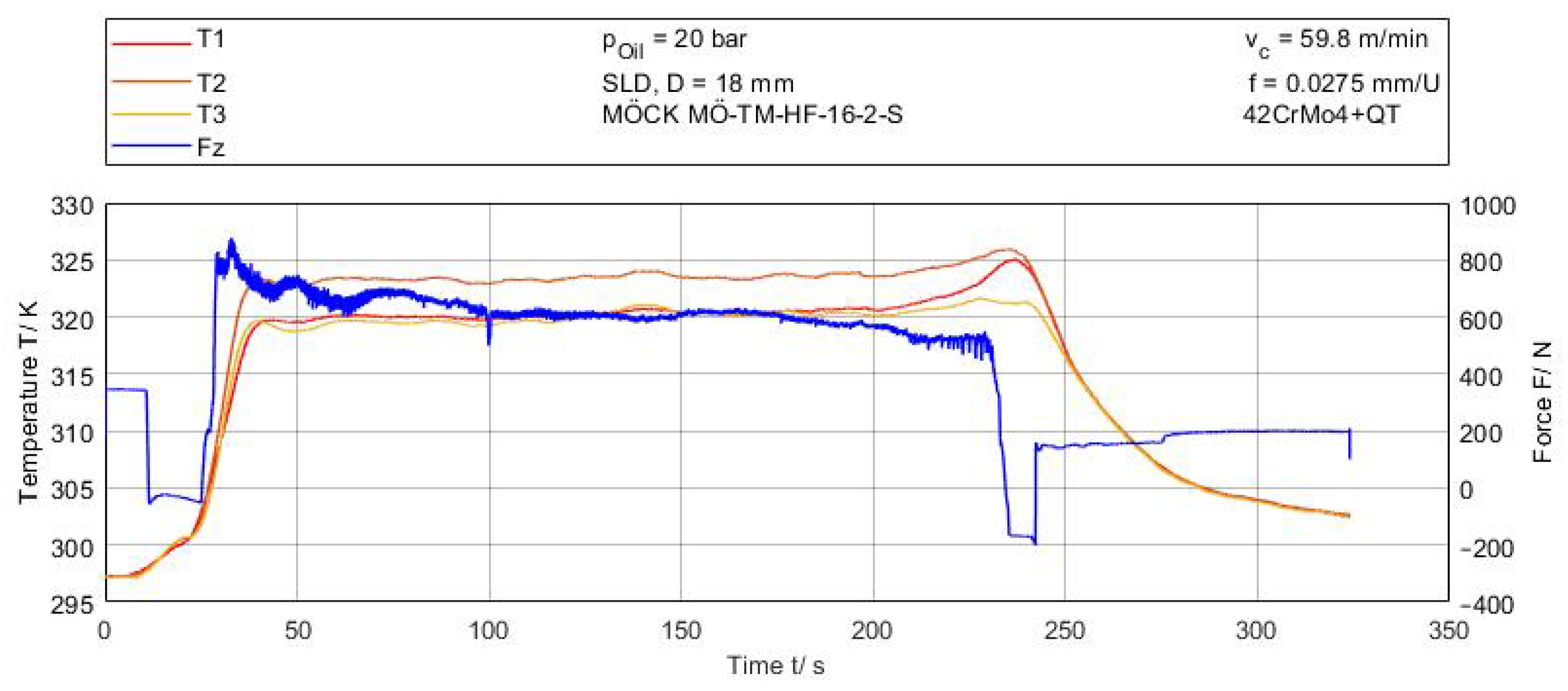
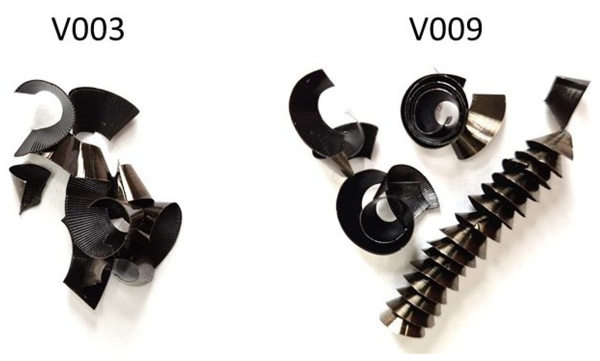
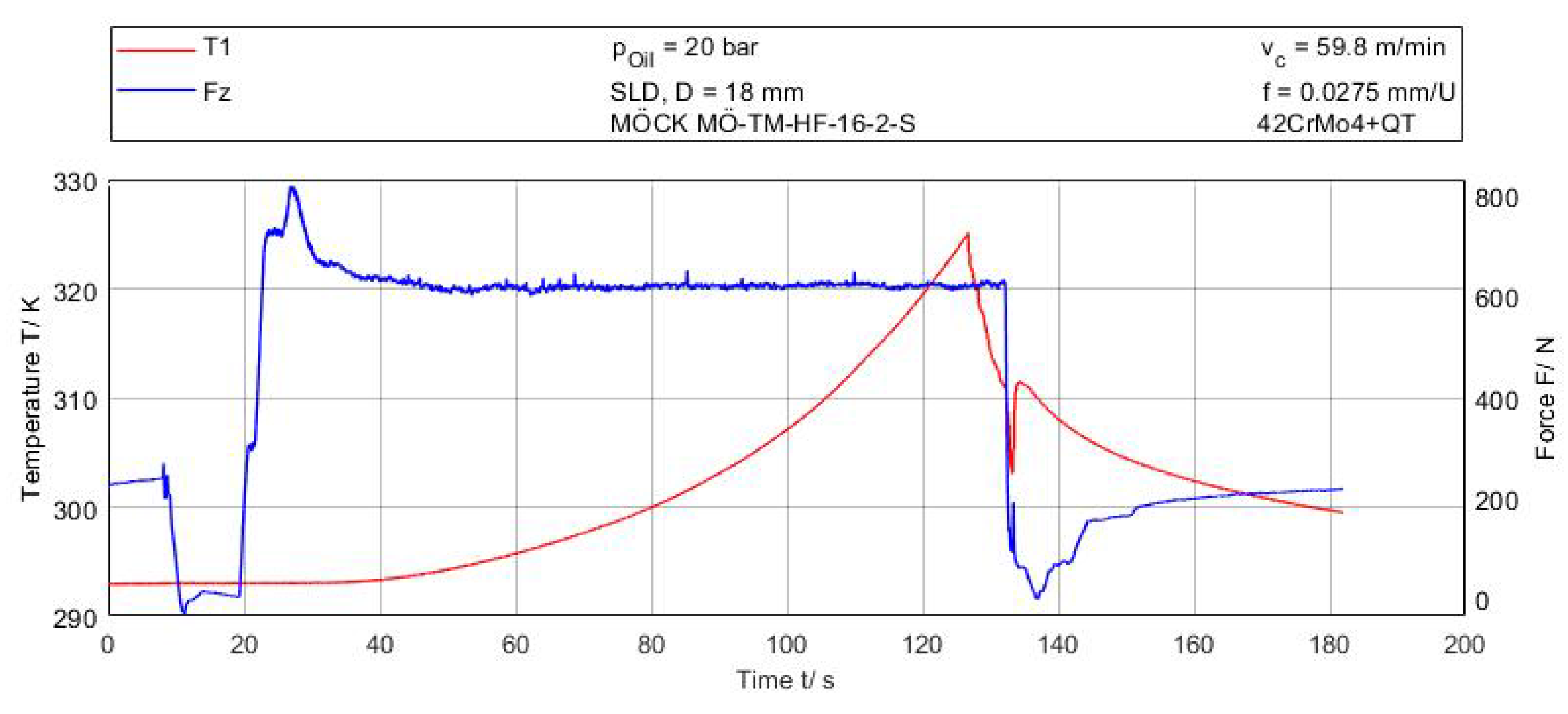
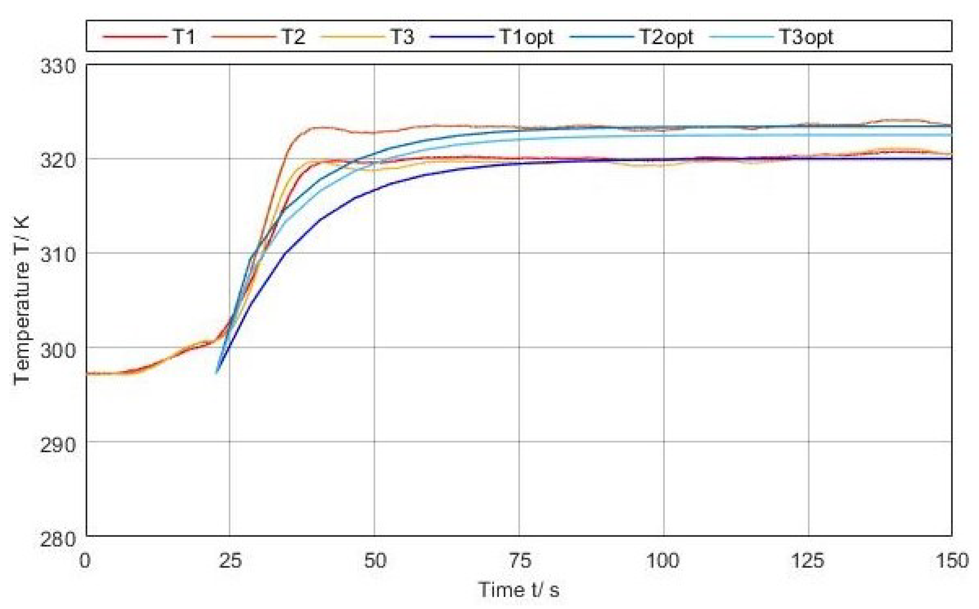
3.3. Experimental Temperature Measurement

The drilling tests are described exemplary on the basis of test $V001$ from the experimental design table, shown in Figure 11. It can be seen that the feed force initially drops since a force opposite to the drilling direction prevails due to the cooling lubricant pressure. Afterwards, a constant force prevails on the tool until it hits the workpiece and the feed force increases. The temperature rise starts at approximately t = 22.5 s with the start of the drilling process. Prior to this, there is a slight temperature increase of $dT$∼ 3 K due to the supply of the drilling oil. Subsequently, the temperature rises within approximately t = 22 s to a constant value of $T_1$ = $T_3$ = 320 K and $T_2$ = 323.5 K, respectively. As the drill-head begins to exit the workpiece, the temperature rises further. Most noticeable is the temperature rise $T_3$ of S3. The sensor S3 is placed with an offset to the rear on the outside of the cutting edge. The drilling oil conveyed through the shank is no longer transported back over the cutting insert due to the absence of the bore ground, but sprays straight out of the tool into the surrounding area. Thus, the cooling effect at the effective point is reduced, while the outer cutting edge oriented in the drilling direction is still engaged. The temperatures at sensors S1 and S3 also undergo a slight temperature increase. This can be explained by the additional heat conducted from the outside of the cutting edge. The more distant the temperature sensor position is, the smaller the temperature rise.

From the effective area diagram in Figure 12, it can be seen that the feed has the most significant effect on the measured temperature. Here, the constant temperature of the sensor S2 during the process was taken into account, since this sensor is the nearest to the effective spot and thus has the highest temperature. The effect of the cutting speed does not provide a clear preview of the course of the temperature. According to this, the temperature is mainly dependent on the feed per revolution. This increases the contact between the chip and the rake face. A greater amount of heat can be transferred into the tool. Whether the contact length increases or longer chips are formed is to be determined by examining the chips. A comparison with the feed force shows a similar behavior of the force and the temperature. The feed force increases as the feed increases. Here, the cutting speed has no particular influence as well.

With an average temperature of T = 328–332 K, the tool in test V003 remains significantly cooler than with T = 340–348 K in V009 although they are produced with the same feeding speed. Accordingly, the same amount of material is machined in the same time. This is also shown by the chip formation. The corresponding chip shapes are shown in Figure 13. The chips obtained in test V003 have an ideally short shape for a safe removal from the effective area. Thus, the heat is quickly taken out of the processing zone. Some of the chips from test V009 roll up considerably. As a result, they tend to remain longer at the effective point, which indicates that more heat can be transferred to the die. In addition, this can lead to a chip hold-up, as a result of which further chips remain in the effective zone.

A process-related advantageous chip shape is therefore also to be preferred for temperature-related reasons. A tool that is colder during the process is not worn as much and therefore has a longer lifetime. The tests were carried out at the same feed rate $v_f$. This results in a difference in the cutting speed $v_c$ and therefore also in the feed f. In addition, the slope of the temperature curve in the area of the warm-up at the beginning of the drilling process was examined. Sensor S2 was also considered, since it is located closest to the point of highest temperature of the cutting edge and thus reacts most directly to the heat transfer by thermal conduction. For this purpose, the effective area diagram shown in Figure 14 was created. Except for one outlier at $v_c$ = 59.82 mm/min and f = 0.0275 mm/rev, the heating rate increases with increasing feed and increasing rotational speed. With a higher feed, more material is machined per revolution. Due to a larger contact area and more energy needed for the formation of the chip, this results in a greater amount of generated and absorbed heat by the tool and chip.

With the approach of temperature measurement via a thermocouple, the absolute temperature of the outer egde of the cutting insert is to be measured. The slow reaction time of the thermocouple is to be relativized by the fact that the thermocouple measures the temperature from the start of the process and so it can gradually heat up with the workpiece, as is shown in Figure 15. In order to measure the temperature as close as possible to the effective point, the thermocouple is machined along with the cutting edge. By the time the thermocouple gets hit by the tool, the temperature either falls, because the thermocouple is pressed out by the cooling lubricant, or the sensor no longer supplies data, as the connection between the two materials is machined.

Based on the process parameters and the sampling rate of the temperature, the maximum occurring distance s between thermocouple and cutting edge can be calculated. This prevails when the cutting edge is slightly less than one time step from the sampling distance of the thermocouple before it is cut. With a set sampling rate of 10 kHz and due to the inertia of the thermocouple, the sensor values are sampled more frequently than new values are written from the sensor. New measured temperature values can be obtained every $t_{delay}$ = 0.16 s. With

$$s=n\times t_{delay}\times f.$$

(8)

the maximum distance where the last temperature is written at is 0.003 mm < s < 0.19 mm. For the investigation of the temperature at the different process parameters from the experimental design, it was also possible to generate an effective area diagram. The effective area diagram from Figure 16 shows, in principle, the same behavior as the temperature measured via the resistance sensors. The measured temperature increases with increasing feed rate. Increasing the cutting speed also leads to an increase in temperature. Here, the impact of the feed rate is not as high as with the sensoric SLD-tool, while the cutting speed has a higher influence on the height of the temperature.

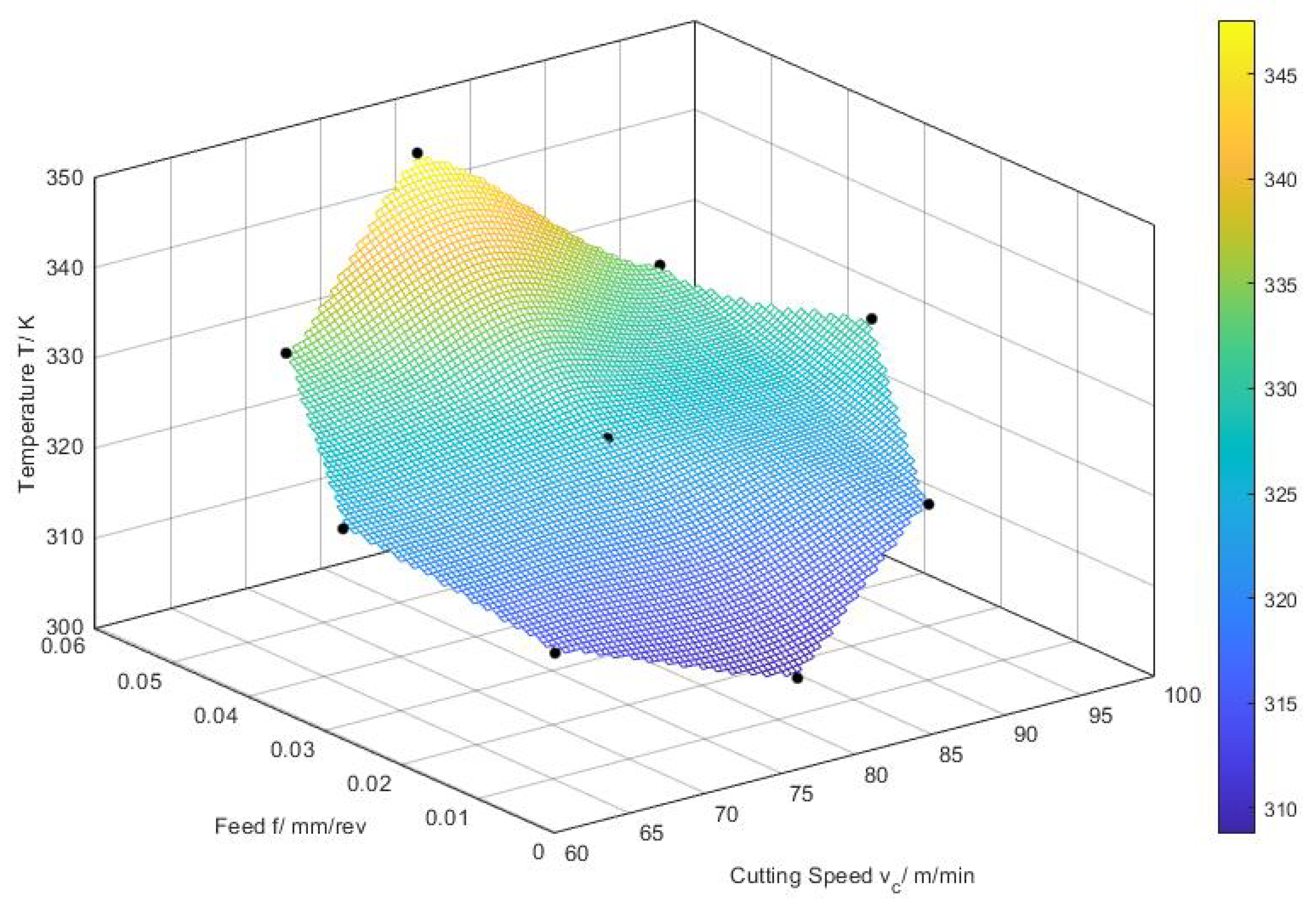
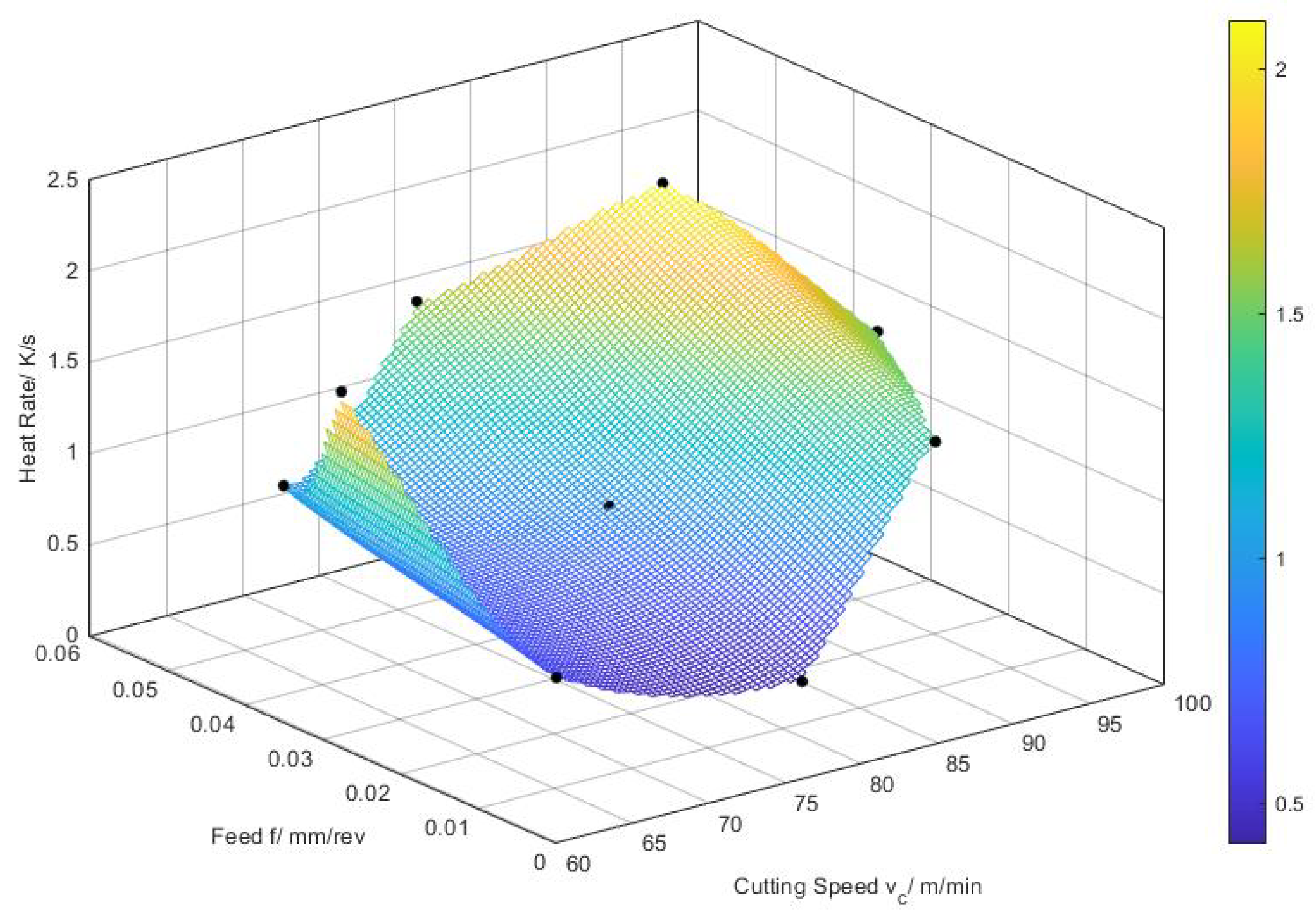
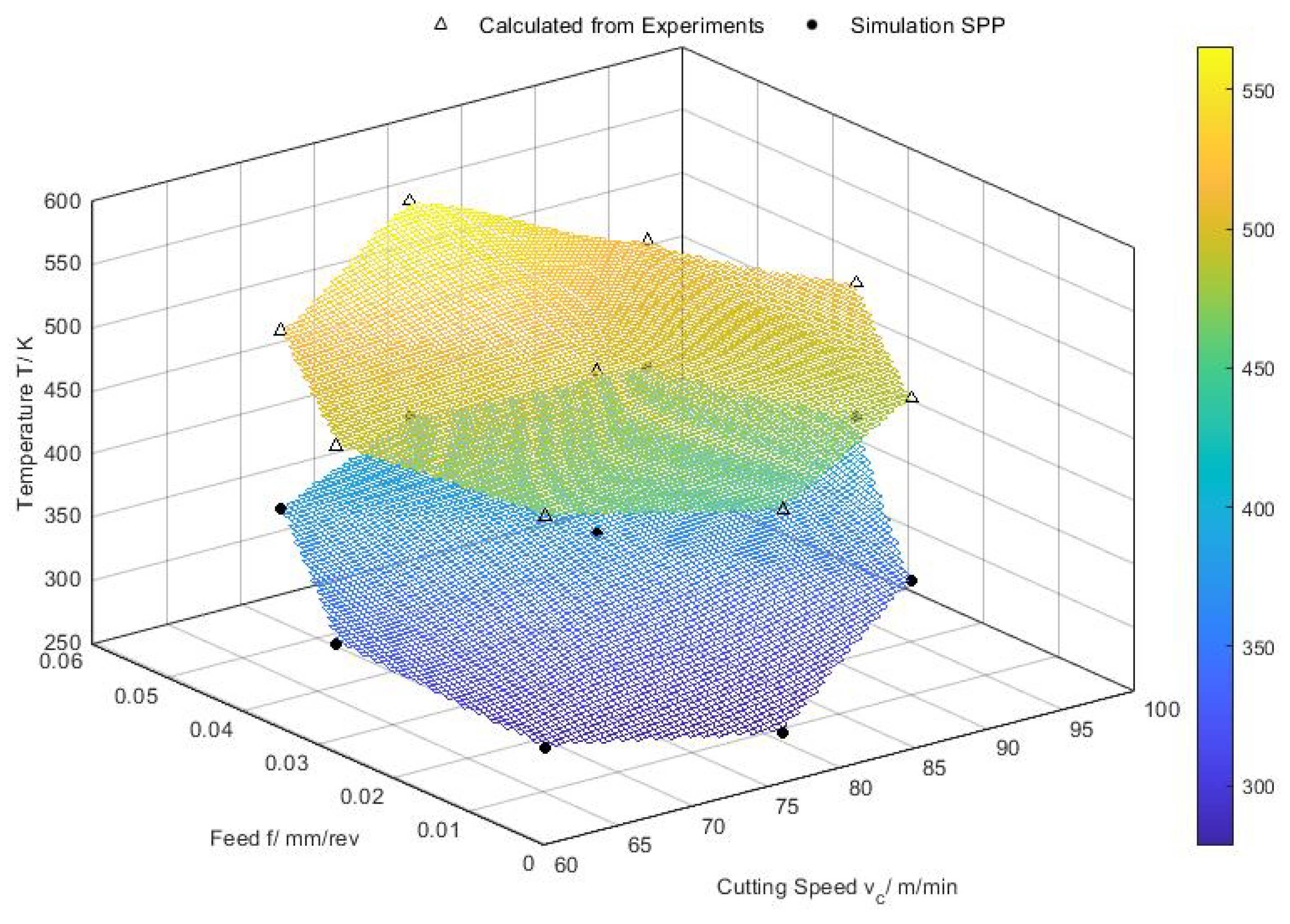
3.4. Calculation of Actual Tool Temperatures

The temperature distribution at the cutting edge can be differentiated between the spot drilling and the drilling process. Since the spot drilling process only represents a short period of the entire drilling process, the following evaluation is related to the constant temperatures during the drilling process. The CEL simulation was carried out with a cutting speed $v_c$ = 80 m/min and a feed f = 0.05 mm/rev. After a simulation time of $t_{sim}$ = 0.5 s, the temperature distribution of the cutting edge was exported. In addition, the geometrical information of the corresponding nodes was read out. Thus, a function can be determined over the cutting edge as a function of the coordinates. The cutting insert is divided into three sections. The first section $T_i$ extends from the tool pivot point to the first cutting edge shoulder. The second section $T_a$ extends further to the cutting edge corner, and the third section $T_f$ represents the outer flank. From the simulation, the following exponential functions are obtained for the sections of the cutting insert:

$$T_i\left(y\right)=1+0.0468e^{0.760y},[0<y<4.81];$$

(9)

$$T_a\left(y\right)=1+0.{305}^{0.281y},[4.81<y<8.83];$$

(10)

$$T_f\left(z\right)=1+31.690e^{0.887z},[2.39<z<10.63];$$

(11)

For test V001, the optimization via Isight results in a factor of k = 89.65. The temperature curves determined by measurement are close to the simulatively calculated temperature curves, as can be seen in Figure 17. Only the start time for the simulated temperature increase has to be offset, since a slight temperature increase in the real drilling process already occurs before the drill affects the workpiece. Therefore, the maximum temperature at the outer edge of the cutting edge is of particular importance since this can influence the properties of the bore hole wall in the form of introduced residual stresses, for example. The function of the second section of the cutting insert results in a temperature of $T_a(Y=8.86)$ = 418 K and the function of the third section results in a temperature of $T_f(Z=2.2)$ = 493.3 K.

The factor k can be represented by a linear influence of the applied temperature to the temperatures at the sensor positions. Thus, the temperatures at the sensors can be calculated in Kelvin by the linear equations as a function of factor k:

$$T_{S1}\left(k\right)=1.778k+160.57;$$

(12)

$$T_{S2}\left(k\right)=2.041k+140.42;$$

(13)

$$T_{S3}\left(k\right)=1.955k+147.28;$$

(14)

From the heat transfer simulation, a temperature increase at sensor position S2 can be determined with a time offset of 0.5 s after the temperature is applied to the cutting edge. The sensors S1 and S3 experience a temperature increase after about 1.7 s.

4. Discussion

From the determination of the temperatures at the outer edge of the cutting insert, a maximum temperature using drilling oil of between 450 K and 570 K is obtained, depending on the process parameters. The temperatures of the tool were investigated with a thermographic camera in a previous work, where no cooling lubricant was used. The highest spot of the temperature in the pictures of the thermografic camera are also at the outer edge of the cutting insert [10]. Compared to measurements of the temperature using a thermographic camera, the temperatures at that spot differ by an amount of about 400 K to 500 K. The difference in the achieved temperatures is mainly due to the use of cooling lubricant. The thermographic measuring method cannot be used in SLD processes with the usage of cooling lubricant, due to the influence of external disturbing factors, such as the exiting cooling lubricant covering the desired measuring area. Therefore, higher temperatures can be measured with the thermographic measuring system.

The use of a cooling lubricant has a significant influence on the temperature of the tool. A steady flow of cooling lubricant changes the frictional conditions and does not produce as much heat at the cutting edge. In addition, hot chips are transported away from the cutting area and there is less heat transfer into the tool. The exact consideration of these factors is very difficult to implement in simulations. The heat transfer from the cutting edge can be taken into account via the factor of natural convection. Different values are given here for different ambient media. The use of the drilling oil “r.rhenus R-OiL DD 10” resembles the properties of mineral oil with an ester content of 5%. From this, the thermal properties closest to the material properties viscosity and density are derived. Thus, the heat transfer coefficient for free thermal convection can be set to a value of $\alpha$ = 108.7 W/m²K for a temperature of 40 °C [17]. The convection that results from the process can also be calculated indirectly from a drilling test that was carried out. During the process, cooling lubricant is fed through the tool at a pressure of p = 20 bar, which corresponds to a flow rate of $\dot{q}$ = 6.1 L/min. Using the model of the temperature distribution at the cutting edge from Section 3.4, the cutting edge is heated to the process temperature. After drilling through the workpiece, the temperature drops because the cutting edge is no longer engaged and is additionally cooled by the fed cooling lubricant through the cooling channel. From this cooling curve, an analysis of the convection after the drilling process can be carried out. Varying the convection heat transfer coefficient results in a value of $\alpha$ = 139.3 W/m${}^2$K for the free convection. In order to be able to determine the convection heat transfer coefficient during the process, the drill must be stopped on the inside of the workpiece. In this way, the coefficient can be determined flow-specifically in further work.

Table 7. Comparison of the thermal convection with literature data.

Heat Transfer Coefficient $\mathit{\alpha }$/W/m${}^2$K	Literature	Optimization
free in air ${\alpha }_{\mathit{air-free}}$	22 [16]	139.3–313.8
air pressure of p = 6 bar ${\alpha }_{ai\mathit{r-}6bar}$	294 [16]	-
free in MQL ${\alpha }_{MQL}$	200–300 [17]	-
drilling oil ${\alpha }_{oil}$	-	further work
emulsion ${\alpha }_{emu}$	5230 [16]	-

presents different values for thermal convection taken from the literature and from the optimization simulations. As the heat transfer coefficient is not a property of the fluid, but is dependent on the fluid properties, the geometry of the probe and the material properties of the probe, a direct comparison is difficult. Kurgin et al. use a thermographic analysis of hollow aluminum cylinders in reaming experiments. With a specific heat capacity of 896 J/kgK, aluminum has a better ability to store heat compared to tungsten carbide. The heat may be kept longer in the material resulting in lower heat transfer coefficients. Because of a higher specific heat and higher thermal conductivity of water in contrast to oil, water based coolants lead to enhanced heat transfer coefficients [16].

No literature values are available for thermal convection for processes using drilling oil under a certain pressure. That is a huge problem in simulations. At the moment, cutting simulations are mostly carried out for dry cutting processes or with an estimated value for the convection heat transfer coefficient of the temperature. In future work, the influence of the drilling oil on the temperature can be considered in more detail.

Neglecting the cooling lubricant in the CEL simulation leads to inaccuracies of the absolute temperature but also of the temperature distribution. A reasonable coupling of the 3D cutting simulation with a fluid simulation representing the cooling lubricant supply is currently not yet reasonable, or merely possible with very high computing power. By neglecting the cooling lubricant, the absolute temperatures of the cutting insert are shifted towards higher temperatures. With the linear adjustment in the back calculation covered in Section 3.4, it may occur that the minimum temperatures decrease below the ambient temperature when looking at the nodes of the center axis of the drill. Here, the assumption must be made that the temperature cannot fall beneath the ambient temperature, but if it does, the calculated temperature has to be set to the ambient temperature. The CEL simulation also features the issue that an engagement of the complete cutting edge leads to convergence problems. The machined material is shifted unfavorably along the bore wall, causing unrealistic temperatures. Accordingly, the simulation time that influences the engagement height of the tool is adjusted to avoid convergence problems and "smearing" of the workpiece material. This leads to deviations in the temperature distribution between the simulation and drilling process. However, the final comparison of the measured temperatures at the sensor positions T1-3 with the corresponding temperatures T1-3opt shows no significant delta, as can be seen in Figure 17. Because the simulation mainly focuses on investigating the temperature distribution with realistic process parameters, there is no particularly nice chip formation to be seen, referred to in Figure 10. The material is removed from the simulation after exiting the Euler room, which represents the chip removal by the drilling oil. The heat conduction from the chip to the tool and corresponding friction conditions are changed. Since the temperature distribution was determined at the nodes of the cutting edge, the effect is negligible considering only the temperatures at the cutting edge for further investigation. Accordingly, not only the methodical procedure is justified, but also the determined analytical equations for the presented process.

A further investigation looking at the correlation between subsurface properties and the thermo-mechanical condition shows a variation of the process parameters in a CEL simulation according to the design of experiments used above. It was shown that the general behavior of the simulation can be correctly approximated in terms of feed force and drilling torque. Figure 18 shows a comparison between the temperature of the calculated CEL simulations and the temperatures determined by the calculation of the temperature at the outer edge of the cutting insert form the sensoriy SLD tool. The general height of the temperature has a delta of $\delta T$ about 100–180 K. Here too, the temperatures of the CEL simulations have a higher gradient [11].

Further investigations can use the equations obtained to calculate a controlling equation that can be used to keep the temperature constant during the process by varying the feed and cutting speed. In this way, the influence of the process temperature with regard to wear and process forces can be considered in more detail and the tool life of deep hole drilling tools can be increased. In addition, by measuring the temperature in the process, a tool wear prediction could be made in order to be able to keep the quality of the bore holes constant. In order to transfer the methodology to tools with other geometries, the presented work can be used as a flow chart. After determining the thermal properties by a defined heat source and setting up a simulation to obtain the analytical temperature distribution at the cutting edge, drilling tests can be performed to determine the temperatures at the respective resistance sensors. By back calculation with the analytical temperature distribution, the temperature at the cutting edge can be concluded.

References

1. Biermann, D.; Bleicher, F.; Heisel, U.; Klocke, F.; Möhring, H.C.; Shih, A. Deep hole drilling. CIRP Ann. 2018, 67, 673–694. [Google Scholar] [CrossRef]
2. Verein Deutscher Ingenieure. VDI 3208: Tiefbohren mit Einlippenbohrern; Verein Deutscher Ingenieure: Düsseldorf, Germany, 2014. [Google Scholar]
3. Wittkop, S. Einlippentiefbohren Nichtrostender Stähle; Schriftenreihe des ISF; Vulkan-Verl.: Essen, Germany, 2007; Volume 40. [Google Scholar]
4. Oezkaya, E.; Baumann, A.; Michel, S.; Schnabel, D.; Eberhard, P.; Biermann, D. Cutting fluid behavior under consideration of chip formation during micro single-lip deep hole drilling of Inconel 718. Int. J. Model. Simul. 2022, 1–15. [Google Scholar] [CrossRef]
5. Davies, M.; Ueda, T.; M’Saoubi, R.; Mullany, B.; Cooke, A. On The Measurement of Temperature in Material Removal Processes. CIRP Ann. 2007, 56, 581–604. [Google Scholar] [CrossRef]
6. Wegert, R.; Alhamede, M.A.; Guski, V.; Schmauder, S.; Möhring, H.C. Sensor-Integrated Tool for Self-Optimizing Single-Lip Deep Hole Drilling. Int. J. Autom. Technol. 2022, 16, 126–137. [Google Scholar] [CrossRef]
7. Möhring, H.C.; Kushner, V.; Storchak, M.; Stehle, T. Temperature calculation in cutting zones. CIRP Ann. 2018, 67, 61–64. [Google Scholar] [CrossRef]
8. Menze, C.; Wegert, R.; Reeber, T.; Erhardt, F.; Moehring, H.C.; Stegmann, J. Numerical methods for the simulation of segmented chips and experimental validation in machining of Ti-6al-4v. MM Sci. J. 2021, 2021, 5052–5060. [Google Scholar] [CrossRef]
9. Wegert, R.; Guski, V.; Möhring, H.C.; Schmauder, S. Determination of thermo-mechanical quantities with a sensor-integrated tool for single lip deep hole drilling. Procedia Manuf. 2020, 52, 73–78. [Google Scholar] [CrossRef]
10. Fandiño, D.; Guski, V.; Wegert, R.; Möhring, H.C.; Schmauder, S. Simulation Study on Single-Lip Deep Hole Drilling Using Design of Experiments. J. Manuf. Mater. Process. 2021, 5, 44. [Google Scholar] [CrossRef]
11. Guski, V.; Wegert, R.; Schmauder, S.; Möhring, H.C. Correlation between subsurface properties, the thermo-mechanical process conditions and machining parameters using the CEL simulation method. Procedia CIRP 2022, 108, 100–105. [Google Scholar] [CrossRef]
12. Nickel, J.; Baak, N.; Volke, P.; Walther, F.; Biermann, D. Thermomechanical Impact of the Single-Lip Deep Hole Drilling on the Surface Integrity on the Example of Steel Components. J. Manuf. Mater. Process. 2021, 5, 120. [Google Scholar] [CrossRef]
13. Nickel, J.; Baak, N.; Walther, F.; Biermann, D. Investigation of the thermomechanical loads on the bore surface during single-lip deep hole drilling of steel components. Procedia CIRP 2022, 108, 805–810. [Google Scholar] [CrossRef]
14. Schermann, T.; Marsolek, J.; Schmidt, C.; Fleischer, J. Aspects of the simulation of a cutting process with ABAQUS/Explicit including the interaction between the cutting process and the dynamic behavior of the dynamic behavior of the machine tool. In Proceedings of the 9th CIRP International Workshop on Modeling of Machining Operations, Bled, Slovenia, 11–12 May 2006. [Google Scholar]
15. Hammelmüller, F.; Zehetner, C. Increasing numerical efficiency in coupled Eulerian-Lagrangian metal forming simulations. In Proceedings of the XIII International Conference on Computational Plasticity. Fundamentals and Applications, COMPLAS XIII, Barcelona, Spain, 1–3 September 2015. [Google Scholar]
16. Kurgin, S.; Dasch, J.; Simon, D.; Barber, G.; Zou, Q. Evaluation of the convective heat transfer coefficient for minimum quantity lubrication (MQL). Ind. Lubr. Tribol. 2012, 64, 376–386. [Google Scholar] [CrossRef]
17. Nadolny, Z.; Dombek, G. Thermal properties of mixtures of mineral oil and natural ester in terms of their application in the transformer. E3S Web Conf. 2017, 19, 01040. [Google Scholar] [CrossRef] [Green Version]
Figure 1. PT1000 temperature sensors S1–3 attached to SLD tool.
Applsci 12 07095 g001
Figure 2. Heat transfer simulation in the cutting insert for determining the heat transfer properties.
Applsci 12 07095 g002
Figure 3. CEL simulation model setup.
Applsci 12 07095 g003
Figure 4. Experimental setup.
Applsci 12 07095 g004
Figure 5. Schematic of the experimental setup for measuring the temperatures in the process zone using a thermocouple.
Applsci 12 07095 g005
Figure 6. Analytical functions describing the temperature distribution on the edge of the cutting insert.
Applsci 12 07095 g006
Figure 7. Temperature evolution of the hot air soldering station experiment.
Applsci 12 07095 g007
Figure 8. (a) Temperature evolution of the heating process, (b) Temperature evolution of the cooling process.
Applsci 12 07095 g008
Figure 9. (a) Orthogonal cut using CEL-method, t s i m = 0.0015 s, v c = 80 m/min, a p = 0.05 mm, mass scale MS = 0 (b) Temperatures of the orthogonal cut with a difference in mesh fineness and mass scaling.
Applsci 12 07095 g009
Figure 10. CEL simulation results, v c = 80 m/min, a p = 0.05 mm, mass scale MS = 10 5 , temperature T /K.
Applsci 12 07095 g010
Figure 11. Temperature T and force F evolution of drilling test V001.
Applsci 12 07095 g011
Figure 12. Effective area diagram of the temperature measured with S2.
Applsci 12 07095 g012
Figure 13. Chip formation of V003 and V009.
Applsci 12 07095 g013
Figure 14. Effective area diagram of the heat rate of S2.
Applsci 12 07095 g014
Figure 15. Temperature measurement via thermocouple V001.
Applsci 12 07095 g015
Figure 16. Effective area diagram of the temperature determined via thermocouple.
Applsci 12 07095 g016
Figure 17. Comparison of the temperature curve V001 of experiment and optimization.
Applsci 12 07095 g017
Figure 18. Comparison of the temperature on the outer edge of the cutting insert.
Applsci 12 07095 g018