Abstract
Light field (LF) cameras can record multi-view images from a single scene, and these images can provide spatial and angular information to improve the performance of image super-resolution (SR). However, it is a challenge to incorporate distinctive information from different LF views. At the same time, due to the inherent resolution of the image sensor, high spatial and angular resolution are trade-off problems. In this paper, we propose a progressive multi-scale fusion network (PMFN) to improve the LFSR performance. Specifically, a progressive feature fusion block (PFFB) based on an encoder-and-decoder structure is designed to implicitly align disparities and integrate complementary information between complementary views. The core module of the PFFB is a dual-branch multi-scale fusion module (DMFM), which can integrate the information from a reference view and auxiliary views to produce a fusion feature. Each DMFM consists of two parallel branches, which have different receptive fields to fuse hierarchical features from complementary views. Three DMFMs with a dense connection are used in the PFFB, which can fully exploit multi-level features to improve the SR performance. Experimental results on both synthetic and real-world datasets demonstrate that the proposed model achieves state-of-the-art performance among existing methods. Moreover, quantitative results show that our method can also generate faithful details.
1. Introduction
Light field (LF) cameras are able to record the spatial and angular information of a scene. This camera technology has been successfully used in many applications, such as VR [1,2], 3D reconstruction [3,4], and saliency detection [5,6]. However, the resolution limitation of camera sensors inhibits the development of LF imaging technology. The higher the angular resolution required of the LF, the lower the spatial resolution obtained for each view. Consequently, LF super-resolution (LFSR) algorithms are widely investigated to retrieve high-resolution (HR) information from low-resolution (LR) images.
Compared with the single image SR (SISR) [7,8], LFSR achieves SR images by using angular and spatial information from different LF views. Based on the complex geometrical structure of LF images, some traditional methods based on disparities have been proposed [9,10]. However, the performance of these methods relies on the accuracy of disparity estimation, and their computational costs are very high. Although optimisation-based methods are constantly researched, obtaining accurate disparities from LR sub-aperture images (SAIs) is still challenging.
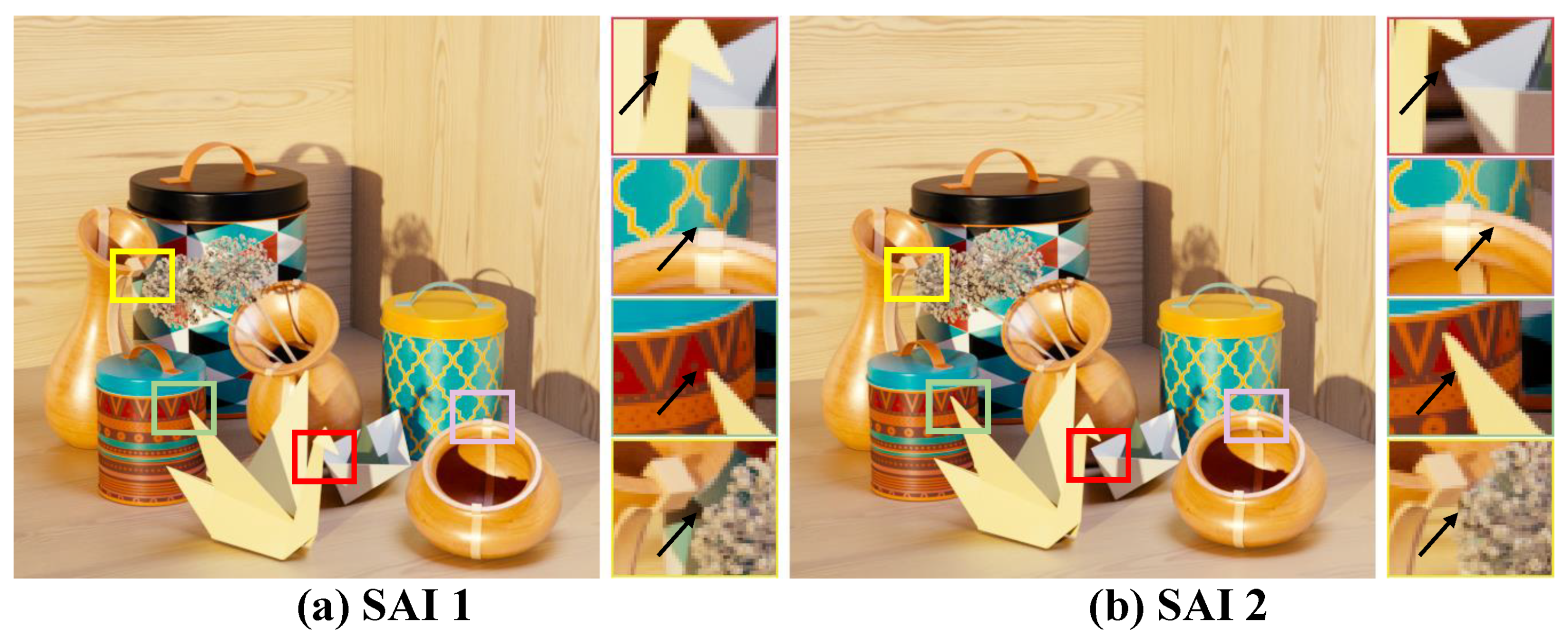
With the development of deep learning, a straightforward way is fine-tuning the network parameters of SISR. However, these methods can hardly preserve the complex 4D structure of LF. Recently, learning-based methods [11,12,13,14,15,16] are utilised to effectively integrate the spatial and angular information, and improve the SR reconstruction. The work in [11] could reconstruct the final high-resolution (HR) SAIs, which simply used the stacked horizontal and vertical directional views. After the structure of the proposed residual network, Zhang et al. [12] proposed the resLFs, which could extract complementary information by stacking the SAIs in four directions. Recently, Jin et al. [13] proposed an all-to-one (ATO) model to generate SR LF images, which combined the reference view and surrounding auxiliary views via combinatorial geometry embedding. Moreover, Wang et al. [14] utilised a different convolution to extract spatial and angular information for LFSR. More recently, Mo et al. [15] designed a view and channel attention to fuse hierarchical features and distillate valid information, which could reconstruct HR LF images. Wang et al. [16] proposed a deformable convolutional network to address the problem of disparities among LF images. Although most of these networks can incorporate spatial and angular information to achieve high accuracy for LF reconstruction, the disparities among different SAIs are still under-investigated. Furthermore, due to the occlusions and non-Lambertian reflections in LF, an image from one view may contain distinctive details compared with images from other views, as shown in Figure 1. The structures of all-to-all networks are not well utilised informative information from auxiliary views for further performance improvement. Consequently, there are two problems existing in LFSR methods, which align the disparities among LF views and supplement the sufficient complementary information.

Figure 1.
Comparison of image content in different SAIs. The location of the two (a) SAI1 and (b) SAI2 are and of the HCI_new named “Origami”. The area indicated by the black arrow shows that the different views contain distinctive information near occlusion edges.
In order to handle these issues, we propose a progressive multi-scale fusion network, PMFN, which has an encoder-and-decoder structure with a progressive multi-scale convolution. Our method is designed to fully use the complementary information from all auxiliary images and implicitly address the problem of disparities among the reference view and auxiliary views. Specifically, we propose a progressive feature fusion block (PFFB) with three dual-branch multi-scale fusion modules (DMFMs). Each DMFM has a dual-branch structure. The two branches of DMFB interact with the extraction feature with different receptive fields, respectively. Then, we concatenate the output features of these two branches with informative information. The PFFB is mainly constructed from three DMFMs. These DMFMs adopt a dense skip connection to strengthen the long-term information from previous DMFMs. Furthermore, this connection can fully exploit hierarchical features and fuse complementary information from auxiliary views. Among these DMFMs, a collect-and-distribute strategy is designed to aggregate informative features from prior DMFMs, and distribute them to the next DMFM. Finally, a feature enhancement block (FEB) is designed to obtain robust SR features. The experimental results on real-world and synthetic datasets demonstrate that our PMFN achieves both higher quantitative and better qualitative performance compared with the state-of-the-art methods. The main contributions of this paper are listed as follows:
- We design the DMFM using a dual-branch structure to implicitly cover the influence of disparities and incorporate informative information from auxiliary views.
- The core PFFB of our network is mainly constructed by three DMFMs with a dense connection. This block can fully exploit multi-level features and the multi-scale fusion information can be preserved among complementary views. It is demonstrated that complementary features are effectively fused by this block to improve SR performance.
- The performance of our PMFN has achieved improvements compared with the state-of-the-art methods developed in recent years.
The rest of this paper is organised into the following sections. Section 2 introduces a brief overview of the related work. Section 3 mainly describes the architecture of our PMFN. In Section 4, we provide extensive analysis, comparative experiments and ablation studies by using synthetic and real-world datasets. Finally, Section 5 summarises the conclusion of this paper.
2. Related Work
In this section, we first review the existing SISR algorithms. Then, some LFSR algorithms are briefly introduced.
2.1. Single Image Super-Resolution
The process of SR is an ill-posed inverse problem, which can reconstruct an HR image. Due to the advantage of deep learning, we briefly review several significant works using deep learning for this task. Among them, Dong et al. [17,18] proposed a seminal network called SRCNN to achieve SISR by utilizing the powerful representation capability of CNN. Compared with the shallow architecture of SRCNN, Kim et al. [8] proposed a residual learning network named VDSR, which mainly learned the high-frequency residual information. Lim et al. [19] proposed an enhanced deep SR network (EDSR), which contained the local and global residual connection. Recently, many SR networks with attention mechanisms had superior performance. Dai et al. [20] proposed a second-order attention network (SAN), which applied the trainable second-order attention module to capture spatial information. To improve the performance of remote-sensing images, Wang et al. [21] proposed a contextual transformation network (CTN), which had a lightweight convolution layer to extract and enrich features. These methods have achieved promising performance in SISR reconstruction. It is noted that the SISR can be applied directly to SR for each SAIs. However, the performance of LFSR is hindered because of the deficient use of complementary information from different views.
2.2. Light Field Super-Resolution
Learning-based methods have greatly improved the performance of LFSR compared to traditional methods. Yoon et al. [22] proposed the LFCNN, which was the first application of deep learning to the LFSR. Inspired by the recurrent convolutional neural network, Wang et al. [11] proposed the LFNet and stacked generalisation technique to synthesise the final SAIs. In this structure, only the structure of horizontal and vertical directional views was used to improve LFSR. Inspired by residual networks, Zhang et al. [12] proposed a residual network (resLF) to extract complementary details from four directions of auxiliary views. The sub-pixel information from auxiliary views was stacked to extract the internal geometric structure relations. In order to maximise the number of auxiliary views, Jin et al. [13] proposed an all-to-one model (ATO) to generate SR LF images via combinatorial geometry embedding. In this structure, the complementary information of each SAIs can be used. Moreover, some effective methods directly calculate angular and spatial dimensions to extract cross-view information. Wang et al. [14] proposed an LF-InterNet to extract and incorporate spatial and angular information. Furthermore, Mo et al. [15] proposed a dense dual-attention network (DDAN) containing a view and channel attention to fuse hierarchical features and distillate valid information. The above methods do not fully deal with the disparity issue among different SAIs. Wang et al. [16] proposed a deformable convolution to incorporate angular information due to disparities among LF images. To fully utilise all angular information, Zhang et al. [23] proposed a multiple epipolar geometry network (MEG-Net), which used multi-direction epipolar images to reconstruct all views images. With the development of Transformer, Wang et al. [24] proposed a detail-preserving Transformer (DPT) to recover the details of LF images by leveraging gradient maps of light field to guide the sequence learning. However, the structures of these methods are all-to-all models, whose complementary information is not well utilised for further performance improvement.
3. Progressive Multi-Scale Fusion Network
Following most existing LFSR methods [13,14,15,16], we only use the Y-channel images as input, which are obtained by converting the RGB-channel images into the YCbCr-channel images, and keeping the Y-channel. Ignoring the channel dimension, the 4D LF can be denoted as , where U, V are angular dimensions, and H, W are spatial dimensions. The process of the LFSR can be described as generating an HR image from an LR image with a spatial resolution of choosing from the angular resolution of . The reconstructed LF images are , where is the upsampling scale. In this section, we introduce our PMFN in detail.
3.1. Overview
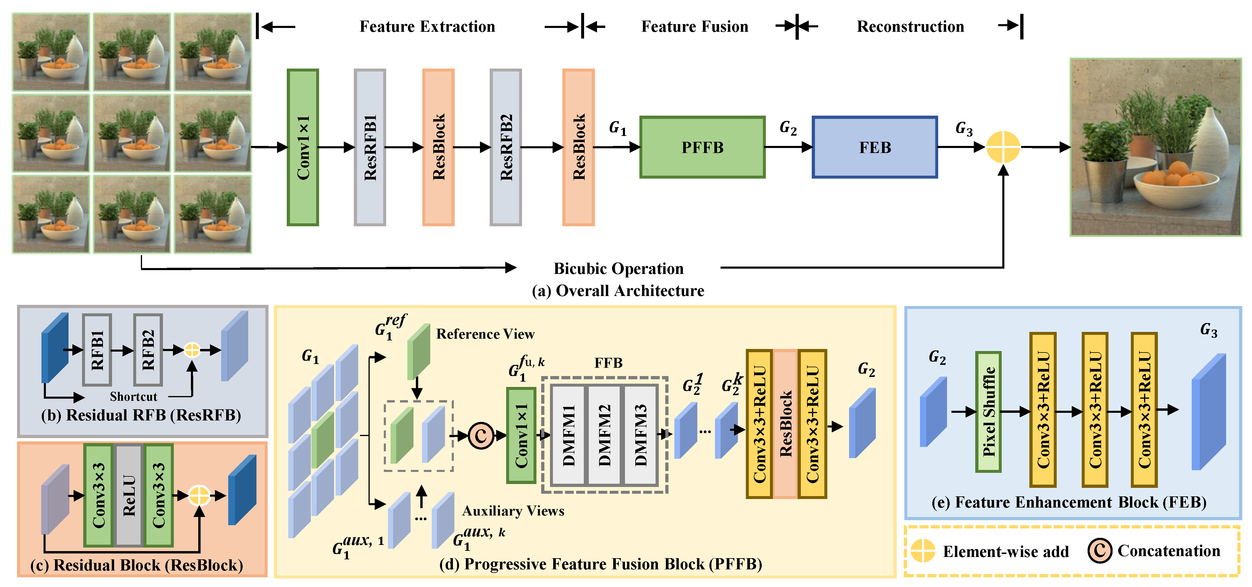
Our PMFN network is shown in Figure 2, which is designed as an all-to-one structure. This network consists of three parts: feature extraction (), feature fusion (), and reconstruction (). Specifically, the residual receptive field block (ResRFB) is designed to extract the shallow features of each SAI, which consists of two RFBs. Given as input, the is first fed to a convolution to generate the initial features. These features are processed by the ResRFB and residual block (ResBlock), respectively. In this part, the shallow features () are extracted by the , which can be expressed by the following,
where represents the shallow features, C is the feature depth, and is the number of SAIs. We divide the into a two part reference-view feature and several auxiliary-view features, which can be expressed as and . Specifically, is arbitrarily selected from and are composed of the remaining features of . The number of is 1 and the number of is . Then, the combined with each of is put into the PFFB, respectively. Notably, the key component of our network is the (PFFB). Through this component, the fusion feature () is generated, connected with informative features of different auxiliary views, i.e.,
where denotes the connection operation, and represents the final fusion feature. After generating the , the feature enhancement block (FEB) is used to bridge the gap between the obtained reference view and the given HR reference view. Then, the residual map () is fine-tuned. This block is very useful to obtain more distillation of valid information and promote more HR reconstruction. The architecture of the FEB is shown in Figure 2e. Finally, the adds a coarse HR image processed by the bicubic interpolation () to generate an HR image (). This process can be simply expressed as
where denotes the residual map, and is an LR reference image, respectively. For other auxiliary views (), they will share the same weights of this network and be combined with different processed by the bicubic interpolation. Eventually, all the HR SAIs are generated, hence the .

Figure 2.
Architecture of the proposed PMFN. The overall network composes of three parts: feature extraction, feature fusion, and reconstruction. The input of our network is LR SAIs. The reference view is randomly selected from these SAIs, and the remaining images are auxiliary view images. The output is an SR reference-view image.
In summary, our all-to-one structure can capture the absent information in the Ref image through other Aux images, which is shown in Figure 3. Moreover, the all-to-all structure can not find unique information from individual views in that the average error over all views is used to optimise during the process of training network [13]. Thus each view in our structure can directly and efficiently incorporate the information from all views.

Figure 3.
Illustration of supplementing complementary information. Here, a () is used as an example. We choose the reference view (), and remaining views are used as auxiliary views. For better comprehension, complementary information from different auxiliary views is visually represented as stars with different colours. Note that the information is added to the blue box in Ref image. The result are shown in the zoomed-in region.
3.2. Residual Receptive Field Block (ResRFB)
Extracting and using discriminative features with rich context information is meaningful to reconstructing HR images with more details. Inspired by [25], we propose the ResRFB to enlarge the receptive field and extract hierarchical features from each LF SAIs. As shown in Figure 4, the RFB consists of the convolutions of different kernel parameters and the dilated convolutions of different dilated rates, which can imitate the human receptive field and increase the diversity of convolution. In the feature extraction part, two RFBs are used with a residual connection. Compared with the atrous spatial pyramid pooling (ASPP) used in [15,16], this block has superior discriminative representation and robustness.

Figure 4.
Architecture of RFB. This block is the basic component of ResRFB.
As shown in Figure 2a, we first put the SAIs into a convolution to extract the initial features. Then, these features are fed into cascaded ResRFBs and ResBlocks, whose structures are shown in Figure 2b,c. The ResRFB is constructed from two identical RFBs and applied with the shortcut design, whose parameter is set to . For each RFB, it has two branches to obtain the hierarchical features, as illustrated in Figure 4. Then, a ReLU activation is used after each ResRFB. For each ResBlock, it consists of two convolutions and a ReLU activation. In summary, multi-scale features of are extracted by using these blocks. The effectiveness of ResRFB is discussed in Section 4.4.
3.3. Progressive Feature Fusion Block (PFFB)
After the feature extraction, the purpose of the PFFB is to implicitly align the disparities between the reference-view and auxiliary-view features. Moreover, this block can effectively exploit the complementary information among LF views. Here, we propose a structure of encoder and decoder, which embeds a progressive receptive field. Figure 2d shows that the basic and core component is the feature-fusion block (FFB), which contains three DMFMs. With this structure, it can map the pairs of features from the reference view and auxiliary views to higher dimensions for fusion by the encoder, and the receptive fields with different scales are suitable for extracting distinctive information from feature maps with different sizes. In this paper, we take t-th DMFMs to perform complementary information fusion. Without loss of generality, the determination of the number of DMFMs is demonstrated in Section 4.4.
As shown in Figure 2d, the reference-view feature is stacked respectively with the auxiliary-view features to construct the feature pairs, and these pairs are first concatenated and fused by a convolution layer in succession. The output of this convolution is . Here, we use t-th DMFMs to generate a fusion feature, which can bring great benefits to implicit feature alignment and feature fusion. The details of the FFB are shown in Figure 5. Specifically, each DMFM has a dual-branch structure mainly consisting of the encoder and decoder convolutions to execute upscaling and downscaling operations. In each branch, we insert two convolutions with different receptive fields in front of the encoder and decoder convolutions to capture the multi-scale information. Then, we concatenate these two branches to obtain the informative high-level feature, . This feature can be specifically expressed as
where represents the operation of our first DMFB, , and the output feature is .
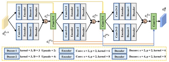
Figure 5.
Architecture of the three DMFMs in the FFB. Specifically, the encoder-and-decoder structure consists of a convolution and a deconvolution. The yellow lines are the input of , the orange lines are the input of , and the blue line is the input of . The structural parameters with different upsampling factors ( and ) are shown in the yellow dotted box.
In our PMFN, three DMFMs are used with a dense connection to fully exploit multi-level features and preserve important information. For the second DMFM, we concatenate and as input and feed them into a convolution to process features. That is,
where is a convolution. Similarly, we can obtain the output of the second DMFM, which is
where denotes the second DMFM. Due to the structure of dense connections, the input of the third DMFM consists of three parts: , , and . We use a convolution to process these features and feed the output into the third DMFM, which can be denoted by
where is a convolution. Finally, we collect the features of different levels from the output of each DMFM and fuse them together by using a convolution. The output of the FFB is , defined as
where is a convolution. The remaining feature pairs, which are constructed by the reference view and each auxiliary view, are produced in the same way, expressed as . To generate the reference feature with other auxiliary views information, we cascade the convolution with a ReLU and a ResBlock, i.e.,
where and denote the convolutions with a ReLU, and is the ResBlock consisting of two convolutions and a ReLU.
As a result, this PFFB can not only supplement complementary-view informative information but also implicitly handles disparities among complementary views. This block is beneficial to improve the fusion ability on complementary views. The effectiveness of the structure of the PFFB is demonstrated in Section 4.4.
3.4. Feature Enhancement Block (FEB)
After generating the fused feature with different auxiliary-view information, this FEB is designed to bridge the gap between the obtained reference view and the given HR reference view. The residual map is fine-tuned by using our FEB. As shown in Figure 2e, the is first proceeded by the pixel shuffle block to generate the coarse feature, which has the same size as . Then, we feed the coarse feature into three cascaded convolutions with a ReLU to refine the HR residual map . That is,
where have the same structure and denote the convolution closely connected to the ReLU. The role of the last is to squeeze the number of the feature channels to 1. Then, the final SR reference image is generated by adding the output of the bicubic operation. This block is very useful to obtain more distillation of valid information and promote more HR reconstruction.
4. Experiments
In this section, we conduct a series of experiments in order to demonstrate the performance of the proposed PMFN. First, we introduce the details of the datasets and the experimental setup. Then, we compare our PMFN to several state-of-the-art SISR and LFSR methods. Finally, we go through the ablation study to investigate the significance of each component in our network.
4.1. Datasets
In this work, we conducted experiments on both synthetic and real-world datasets. It is more meaningful for LF algorithms to adapt to different datasets with different scenes. As listed in Table 1, HCInew [26], HCIold [27], EPFL [28], INRIA [29], and STFgantry [30] are the six public LF datasets we use, each having different characteristics. STFgantry has the largest LF disparity, including the most distinctive information between two adjacent views compared with other datasets. EPFL, INRIA, and STFgantry are captured by the Lytro Illum cameras, consisting of real-world scenes. Each dataset is divided into the training and testing parts. Specifically, 144 LF images were used for training and 23 LF images were used for testing our method. The original SAIs of LF for these datasets have an angular resolution of .

Table 1.
Public LF datasets used in our experiments.
4.2. Settings and Implementation Details
To generate the LR LF images, the bicubic downsampling method is used to generate LR patches, with and downsampling factors. Our PMFN sets the channel number of features to 64. The patch size is set to . The resolutions of the angular and spatial are and , respectively. These LF images are randomly processed by flipping the images horizontally or vertically and rotating them 90 degrees. Our network adopts the L1 Loss function and Adam optimiser (, ). The initial learning rate was set to 1 × 10 and decreased by a factor of 0.5 every 250 epochs. The total training steps are set at 400 epochs. We trained our network with NVIDIA RTX 2080 TI GPU, and this model is based on the PyTorch framework.
4.3. Comparison to the State of the Art
We compare the results of the PMFN with recent state-of-the-art single image SR (SISR) and LFSR methods, which are VDSR [8], EDSR [19], GB [31], resLF [12], LFSSR [32], LF-ATO [13], LF-InterNet [14], LF-DFNet [14], MEG-Net [23], and DPT [24]. The bicubic method is the baseline of comparison. The VDSR and EDSR are the typical methods for SISR. The GB is the traditional method for LFSR. The resLF, LFSSR, LF-ATO, LF-InterNet, LF-DFNet, MEG-Net, and DPT are the LFSR methods by using deep learning. The learning-based methods have been retrained on the same training datasets for consistency. Meanwhile, we used peak signal-to-noise ratio (PSNR) and structural similarity (SSIM) to evaluate the quantitative performance.
4.3.1. Quantitative Results
As shown in Table 2, the quantitative results have a LF views for SR and SR. These results show that our approach is comparable with the state-of-the-art SR methods. We also notice that our network achieves the best performance on EPFL, INRIA, and STFgantry datasets. The best results are shown in red and the second results are shown in blue. In Table 2, the value of PSNR (SSIM) of our PMFN far exceeds that of EDSR in STFgantry, which differs by 3.73 dB (0.011) in terms of PSNR (SSIM) for SR. That is because these SISR methods ignore the complementary information existing in other views, which limits the performance of SR. Compared with the traditional LFSR method (GB), our method has 3.97 dB (0.041) higher in terms of PSNR (SSIM) for SR. Our method is based on deep CNNs to achieve better performance compared with GB, which benefits from the representation learning capability of CNN. The average PSNR (SSIM) results of all testing scenes for LF-DFNet, MEG-Net, DPT, and our method are 31.32 dB (0.934), 31.72 dB (0.937), 31.56 dB (0.940), and 31.97 dB (0.940) for the task, respectively. Note that it can be observed that our PMFN has the best generalisation among all datasets. The performance of our network is mediocre in HCInew and HCIold. That is because our network implicitly addresses the influence of disparities by using multiple receptive fields to capture the corresponding pixels, which is not suitable for disparities in the middle. In summary, our method can incorporate complementary information among different views, especially in small and large disparity datasets (EPFL, INRIA, and STFgantry).
Table 2.
PSNR/SSIM values achieved by different methods for and SR, the best results are in red and the second best results are in blue.
4.3.2. Qualitative Results
Figure 6 is the qualitative results for and SR. Compared with the state-of-the-art SISR and LFSR methods, it can be seen that our model effectively generates not only faithful details but fewer artefacts. Specifically, we achieve better performance of stairway in scene INRIA_Sculpture visual quality for SR. We also notice that our approach is able to recover challenging scenes due to the occlusions and complex scenes, such as STFgantry_Cards for SR. In general, our method can effectively reconstruct LF images.
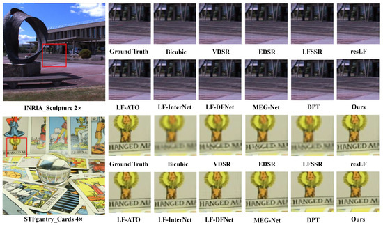
Figure 6.
Visual comparisons of different methods on and reconstruction.
4.3.3. Parameters and FLOPs
In Table 3, we compare the number of parameters (Param.), FLOPs, and the average of PSNR and SSIM (Avg. PSNR/SSIM) between our PMFN and other LFSR methods on testing datasets for 4× upscaling. Note that our method consumes little computational efficiency but achieves the best results compared with SISR and LFSR methods, especially for the reference view. Furthermore, our PMFN has fewer parameters and better performance than DPT [24]. In summary, our method has a good performance not only on the performance of the model but also on the scores of PSNR and SSIM.
Table 3.
The comparative results in terms of the number of parameters, FLOPSs, and average PSNR/SSIM on testing sets for LF image SR methods. FLOPs are calculated on 5 × 5 × 32 × 32 input features.
4.4. Ablation Study
We conducted extensive comparative experiments to verify the contributions of different components in our PMFN, including the ResRFB for feature extraction, the FFB for feature fusion and the FEB for reconstruction. As shown in Figure 7, they are visual results with different variants. It is demonstrated that our designed network can achieve the best SR performance. Meanwhile, we investigate the performance of different numbers of DMFM and the influence of the connection mode in our FFB.
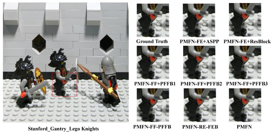
Figure 7.
Visual results of different variants of our network on “Stanford_Gantry_Lego Knights” for visual SR.
PMFN-FE w/o ResRFB: The ResRFB is used to extract multi-scale initial features in feature extraction. We investigated the benefit of this block through these two experiments (PMFN-FE + ASPP and PMFN-FE + ResBlock). In order to ensure the parameters of these networks are similar, we introduce two blocks (ASPP and ResBlock) to replace the part of ResRFB to extract the features. As shown in Table 4, the value of the average PSNR is decreased by 0.18 and 0.32 for SR in EPFL, HCInew, HCIold, INRIA, and STFgantry datasets, respectively. Compared with ResBlock and ASPP, our ResRFB has progressive receptive fields, which are beneficial to extract hierarchical features.
Table 4.
PSNR/SSIM values achieved by PMFN and its variants for SR.
Number of DMFMs: This component is the key to our network to achieve feature fusion. Table 5 shows the computational efficiency and quality of the reconstruction affected by different amounts of our DMFMs. It can be observed that the accuracy consistently improves as the number of DMFMs increases. However, the computational efficiency continues to decline and the performance is not significant. It can be observed that the values of PSNR are very similar when the number of DMFMs is between three and five. In this paper, we decided to set three DMFMs to achieve a meaningful trade-off between computational efficiency and the quality of reconstruction.
Table 5.
The comparative results of different number of DMFMs on the EPFL for LFSR.
Structure of FFB: We compare the SR performance with different architectures of PFFB. As shown in Figure 8, it demonstrates the different structures based on DMFM. We adopt three DMFMs to investigate the effectiveness of our structure. Compared with the FFB, the structure of the FFB1 is only three cascaded DMFMs, there is no other way to achieve connection. This variant suffers a decrease of 0.48 dB as compared to PMFN. The FFB2 removes the branches of the input feature, which suffers a decrease of 0.16 dB as compared to PMFN. These two demonstrate the effectiveness of dense connection in PMFN. Although the FFB3 and FFB have the same structure, the FFB3 removes the progressive multi-scale convolution. This result suffers a decrease of 0.42 dB as compared to PMFN. Moreover, we remove our FFB in the variant of the PMFN-FF - FFB to investigate this contribution. This result suffers the worst decrease of 0.79 dB in all variants. Our three DFFMs with dense connections can achieve better performance. That is because both low-level and high-level features are beneficial to the SR performance, and progressive multi-scale design can improve feature representation and enlarge the receptive fields.

Figure 8.
Different structures of the FFB. FFB1 uses a straight forward connection, FFB2 uses a dense connection without introducing input features, FFB3 uses a dense connection without multi-scale features, and FFB is the structure used in our network.
Structure of FEB: The FEB is used in our PMFN for high-frequency details reconstruction. To demonstrate its effectiveness, we remove the middle two cascaded convolutions with a ReLU and only preserve the last convolution. The result (PMFN-FF-FEB) is lower than PMFN (0.05 dB). That is because the high-frequency features of HR images have been further fine-tuned.
Number of angular resolution: We also analyse the performance of our PMFN in different SAIs. We used , and SAIs in both synthetic (STFgantry) and real-world (HCInew) datasets. As shown in Table 6, the values of PSNR and SSIM can be improved as the number of angular resolutions increases. That is because more complementary information is fused into the reference view with angular resolution increases. In this paper, all results compared with state-of-the-art are obtained with SAIs, because these SAIs are enough to investigate the efficiency of our method.
Table 6.
Comparative results of different angular resolutions on the STFgantry and HCInew using our PMFN for and LFSR.
5. Conclusions
In this paper, we propose an all-to-one network PMFN for LFSR. To make full use of complementary information between the reference view and auxiliary views, we design a PFFB with three densely connected DMFMs. This block can implicitly deal with disparities among different views. Additionally, in this block, low-level and high-level features are incorporated to improve the SR performance. Moreover, we design an FEB to further refine the HR residual map to improve the SR reference view. Experimental results have demonstrated the superiority of our PMFN over other state-of-the-art methods.
In future work, an adaptive receptive field network can be investigated to improve the accuracy of generated texture details. This network should adapt to different disparities, and have generalization in synthetic and real-world datasets.
Author Contributions
Conceptualization, W.Z.; methodology, W.Z., W.K., H.S. and Z.X.; writing—original draft preparation, W.Z.; writing—review and editing, W.Z., W.K., H.S. and Z.X.; Funding acquisition, W.K., H.S. and Z.X. All authors have read and agreed to the published version of the manuscript.
Funding
This study was partially supported by the National Key R&D Program of China (2018YFB2101100), the National Natural Science Foundation of China (61872025), the Science and Technology Development Fund, Macau SAR (0001/2018/AFJ) and the Open Fund of the State Key Laboratory of Software Development Environment (SKLSDE-2021ZX-03).
Institutional Review Board Statement
Not applicable.
Informed Consent Statement
Not applicable.
Data Availability Statement
Not applicable.
Conflicts of Interest
The authors declare no conflict of interest.
References
- Huang, F.; Chen, K.; Wetzstein, G. The light field stereoscope. ACM Trans. Graph. 2015, 34, 1–12. [Google Scholar]
- Yu, J. A light-field journey to virtual reality. IEEE MultiMedia 2017, 24, 104–112. [Google Scholar] [CrossRef]
- Kim, C.; Zimmer, H.; Pritch, Y.; Sorkine-Hornung, A.; Gross, M.H. Scene reconstruction from high spatio-angular resolution light fields. ACM Trans. Graph. 2013, 32, 73. [Google Scholar] [CrossRef]
- Zhu, H.; Wang, Q.; Yu, J. Occlusion-model guided antiocclusion depth estimation in light field. IEEE J. Sel. Top. Signal Process. 2017, 11, 965–978. [Google Scholar] [CrossRef] [Green Version]
- Piao, Y.; Li, X.; Zhang, M.; Yu, J.; Lu, H. Saliency detection via depth-induced cellular automata on light field. IEEE Trans. Image Process. 2019, 29, 1879–1889. [Google Scholar] [CrossRef] [PubMed]
- Zhang, M.; Li, J.; Wei, J.; Piao, Y.; Lu, H.; Wallach, H.; Larochelle, H.; Beygelzimer, A.; d’Alche Buc, F.; Fox, E. Memory-oriented Decoder for Light Field Salient Object Detection. In Proceedings of the NeurIPS, Vancouver, BC, Canada, 8–14 December 2019; pp. 896–906. [Google Scholar]
- Zhang, Y.; Li, K.; Li, K.; Wang, L.; Zhong, B.; Fu, Y. Image super-resolution using very deep residual channel attention networks. In Proceedings of the European Conference on Computer Vision (ECCV), Munich, Germany, 8–14 September 2018; pp. 286–301. [Google Scholar]
- Kim, J.; Kwon Lee, J.; Mu Lee, K. Accurate image super-resolution using very deep convolutional networks. In Proceedings of the IEEE Conference on Computer Vision and Pattern Recognition, Las Vegas, NV, USA, 27–30 June 2016; pp. 1646–1654. [Google Scholar]
- Wanner, S.; Goldluecke, B. Variational light field analysis for disparity estimation and super-resolution. IEEE Trans. Pattern Anal. Mach. Intell. 2013, 36, 606–619. [Google Scholar] [CrossRef] [PubMed]
- Farrugia, R.A.; Galea, C.; Guillemot, C. Super resolution of light field images using linear subspace projection of patch-volumes. IEEE J. Sel. Top. Signal Process. 2017, 11, 1058–1071. [Google Scholar] [CrossRef] [Green Version]
- Wang, Y.; Liu, F.; Zhang, K.; Hou, G.; Sun, Z.; Tan, T. LFNet: A novel bidirectional recurrent convolutional neural network for light-field image super-resolution. IEEE Trans. Image Process. 2018, 27, 4274–4286. [Google Scholar] [CrossRef] [PubMed]
- Zhang, S.; Lin, Y.; Sheng, H. Residual networks for light field image super-resolution. In Proceedings of the IEEE/CVF Conference on Computer Vision and Pattern Recognition, Long Beach, CA, USA, 15–20 June 2019; pp. 11046–11055. [Google Scholar]
- Jin, J.; Hou, J.; Chen, J.; Kwong, S. Light field spatial super-resolution via deep combinatorial geometry embedding and structural consistency regularization. In Proceedings of the IEEE/CVF Conference on Computer Vision and Pattern Recognition, Seattle, WA, USA, 13–19 June 2020; pp. 2260–2269. [Google Scholar]
- Wang, Y.; Wang, L.; Yang, J.; An, W.; Yu, J.; Guo, Y. Spatial-angular interaction for light field image super-resolution. In Proceedings of the European Conference on Computer Vision, Glasgow, UK, 23–28 August 2020; Springer: Berlin/Heidelberg, Germany, 2020; pp. 290–308. [Google Scholar]
- Mo, Y.; Wang, Y.; Xiao, C.; Yang, J.; An, W. Dense Dual-Attention Network for Light Field Image Super-Resolution. IEEE Trans. Circuits Syst. Video Technol. 2021, 32, 4431–4443. [Google Scholar] [CrossRef]
- Wang, Y.; Yang, J.; Wang, L.; Ying, X.; Wu, T.; An, W.; Guo, Y. Light field image super-resolution using deformable convolution. IEEE Trans. Image Process. 2020, 30, 1057–1071. [Google Scholar] [CrossRef] [PubMed]
- Dong, C.; Loy, C.C.; He, K.; Tang, X. Learning a deep convolutional network for image super-resolution. In Proceedings of the European Conference on Computer Vision, Zurich, Switzerland, 6–12 September 2014; Springer: Berlin/Heidelberg, Germany, 2014; pp. 184–199. [Google Scholar]
- Dong, C.; Loy, C.C.; He, K.; Tang, X. Image super-resolution using deep convolutional networks. IEEE Trans. Pattern Anal. Mach. Intell. 2015, 38, 295–307. [Google Scholar] [CrossRef] [PubMed] [Green Version]
- Lim, B.; Son, S.; Kim, H.; Nah, S.; Mu Lee, K. Enhanced deep residual networks for single image super-resolution. In Proceedings of the IEEE Conference on Computer Vision and Pattern Recognition Workshops, Honolulu, HI, USA, 21–26 July 2017; pp. 136–144. [Google Scholar]
- Dai, T.; Cai, J.; Zhang, Y.; Xia, S.T.; Zhang, L. Second-order attention network for single image super-resolution. In Proceedings of the IEEE/CVF Conference on Computer Vision and Pattern Recognition, Long Beach, CA, USA, 15–20 June 2019; pp. 11065–11074. [Google Scholar]
- Wang, S.; Zhou, T.; Lu, Y.; Di, H. Contextual Transformation Network for Lightweight Remote-Sensing Image Super-Resolution. IEEE Trans. Geosci. Remote Sens. 2021, 60, 1–13. [Google Scholar] [CrossRef]
- Yoon, Y.; Jeon, H.G.; Yoo, D.; Lee, J.Y.; So Kweon, I. Learning a deep convolutional network for light-field image super-resolution. In Proceedings of the IEEE International Conference on Computer Vision Workshops, Santiago, Chile, 7–13 December 2015; pp. 24–32. [Google Scholar]
- Zhang, S.; Chang, S.; Lin, Y. End-to-end light field spatial super-resolution network using multiple epipolar geometry. IEEE Trans. Image Process. 2021, 30, 5956–5968. [Google Scholar] [CrossRef] [PubMed]
- Wang, S.; Zhou, T.; Lu, Y.; Di, H. Detail preserving transformer for light field image super-resolution. In Proceedings of the AAAI Conference on Artificial Intelligence, Virtual, 22 February–1 March 2022. [Google Scholar]
- Liu, S.; Huang, D. Receptive field block net for accurate and fast object detection. In Proceedings of the European Conference on Computer Vision (ECCV), Munich, Germany, 8–14 September 2018; pp. 385–400. [Google Scholar]
- Honauer, K.; Johannsen, O.; Kondermann, D.; Goldluecke, B. A dataset and evaluation methodology for depth estimation on 4d light fields. In Proceedings of the Asian Conference on Computer Vision, Taipei, Taiwan, 20–24 November 2016; Springer: Berlin/Heidelberg, Germany, 2016; pp. 19–34. [Google Scholar]
- Wanner, S.; Meister, S.; Goldluecke, B. Datasets and benchmarks for densely sampled 4D light fields. In Proceedings of the Vision, Modeling and Visualization (VMV 2013), Lugano, Switzerland, 11–13 September 2013; Volume 13, pp. 225–226. [Google Scholar]
- Rerabek, M.; Ebrahimi, T. New light field image dataset. In Proceedings of the 8th International Conference on Quality of Multimedia Experience (QoMEX), Lisbon, Portugal, 6–8 June 2016. [Google Scholar]
- Le Pendu, M.; Jiang, X.; Guillemot, C. Light field inpainting propagation via low rank matrix completion. IEEE Trans. Image Process. 2018, 27, 1981–1993. [Google Scholar] [CrossRef] [PubMed] [Green Version]
- Vaish, V.; Adams, A. The (New) Stanford Light Field Archive; Computer Graphics Laboratory, Stanford University: Stanford, CA, USA, 2008; Volume 6. [Google Scholar]
- Rossi, M.; Frossard, P. Geometry-consistent light field super-resolution via graph-based regularization. IEEE Trans. Image Process. 2018, 27, 4207–4218. [Google Scholar] [CrossRef] [PubMed] [Green Version]
- Yeung, H.W.F.; Hou, J.; Chen, X.; Chen, J.; Chen, Z.; Chung, Y.Y. Light field spatial super-resolution using deep efficient spatial-angular separable convolution. IEEE Trans. Image Process. 2018, 28, 2319–2330. [Google Scholar] [CrossRef] [PubMed]


Publisher’s Note: MDPI stays neutral with regard to jurisdictional claims in published maps and institutional affiliations. |
© 2022 by the authors. Licensee MDPI, Basel, Switzerland. This article is an open access article distributed under the terms and conditions of the Creative Commons Attribution (CC BY) license (https://creativecommons.org/licenses/by/4.0/).