Numerical Analysis on Self-Propulsion of a Waterjet-Propelled Ship with Different Propulsion Models

Abstract

The hydrodynamics of the waterjet-propelled ship is a challenging issue due to the sophistication of waterjet system geometry as well as waterjet–hull interaction. In current study, three different propulsion models, namely, multiple reference frame (MRF) model, sliding mesh model and body-force model, are utilized to simulate the self-propulsion of a waterjet-propelled ship model. A body-force model based on a User-Defined Function (UDF) on the ANSYS Fluent platform is proposed. The computational cost, wave pattern, jet stream surface, and self-propelled hull resistance of the MRF model and body-force model are compared. Comprehensive comparisons of the internal ingested flow field of the control volume are made, especially at the capture area and nozzle section, with the two different models. In addition, the resistance increment fraction and jet system thrust deduction fraction with the two different models are investigated. Lastly, the flow field with the steady MRF model, the body-force model (RANS) and the transient sliding mesh model (URANS) are compared.

1. Introduction

Currently, waterjet propulsion has attracted much interest attributed to its advantages of shallow draft, lower noise, less vibration, etc., compared with conventional screw propellers. Consequently, the accurate prediction and in-depth analysis of the hydrodynamics for a waterjet-propelled ship have become the concern of researchers. The main research methods adopted in the field of waterjet propulsion include theoretical analysis, experimental measurement and numerical simulation.

In the early 1990s, a series of colloquiums [1,2,3,4,5,6,7,8,9] on the waterjet propulsion system and waterjet–hull interaction were launched by the ITTC Specialist Committee. The 23rd ITTC Specialist Committee on the validation of waterjet test procedures formulated a model testing procedure for waterjet propulsion. Figure 1 shows the ITTC control volume standard locations for the waterjet flow, where station 1a for inflow capture area is situated one pump diameter in front of the inlet tangency point, station 3 is located just ahead of the pump, and station 6 is at the nozzle discharge.

In the past, the interaction between propeller and hull for ships with conventional screw propellers has been widely studied in previous researches, while for waterjet-propelled ships, the waterjet system is embedded in the hull, so the interaction between waterjet and hull is still a challenging problem. Coop [10] studied the waterjet–hull interaction effects, measured the thrust deduction, and established an analytical propulsion model to include the waterjet momentum forces. Van Terwisga [11] investigated the waterjet–hull interaction comprehensively with theoretical analysis, experimental measurement and numerical simulation. Bulten [12] performed experimental and numerical investigations, and found an obvious deviation between the force yielded by integrating the axial force component and the thrust obtained by the simplified momentum balance equation.

Computational Fluid Dynamics (CFD) techniques make it more effective and efficient to investigate the waterjet–hull interaction, especially in recent years. Delaney et al. [13] analyzed the waterjet pump characteristics for a Joint High Speed Sealift (JHSS) hull by RANS computations, and mentioned the momentum non-uniformity factor. Kandasamy et al. [14] derived an integral force/moment waterjet model to predict the ship local flow variables by CFDSHIP-IOWA solver. Takai et al. [15] applied the unsteady Reynolds-Averaged Navier–Stokes (URANS) CFDSHIP-IOWA solver to simulate the flow field of a bare hull and the self-propelled conditions. Eslamdoost et al. [16] presented a fast and robust method, called the pressure jump method, to simulate the waterjet–hull interaction with potential flow theory. The main parameters affecting the waterjet–hull interaction were also determined in his doctoral thesis [17]. Furthermore, Eslamdoost et al. [18] employed numerical simulations to study the relation between net thrust and gross thrust. They used CFD to address the large variation of water thrust deduction with Froude number [19]. The impact on the external flow field could further affect the momentum velocity coefficient, which was an important evaluation index of the waterjet–hull interaction [20]. Liu and Chen [21] found that the non-uniform inflow reduced the external characteristics of the waterjet pump and led to the huge fluctuation of energy performance with time. Guo et al. [22] adjusted the impeller rotational speed to balance the horizontal force of the waterjet-propelled trimaran, and then determined the self-propulsion point. Ji et al. [23] studied the effect of improving the blade tip size in pump-jet propulsor through CFD numerical simulation. Jiang and Ding [24] studied the hull–waterjet interaction of a planning trimaran, including analysis of thrust deduction and interaction efficiency. They also conducted detailed investigations on the respective effect of waterjet suction and jet action on hull resistance with Froude Number, as well as the effect of hull displacement on the hydrodynamics for the same planning trimaran [25,26]. Gong et al. [27] investigated the stabilizer fin’s influence on the flow fields of a waterjet-propelled ship, including the boundary layer distribution around the hull and the momentum velocity coefficient at station 1a.

For ships with conventional propellers, there have been many studies on propeller rotation models in recent years, mainly including the discretized propeller model and the body-force model based on the open water curve of propeller [28,29,30,31,32,33]. However, for a waterjet propulsion system with complex geometric structure, it is necessary to consider the comprehensive effect of the flow channel, impeller and guide vane in the momentum control volume, not just the open water curve of the impeller. Two common methods for the numerical simulation of pump system are the real pump geometric model and body-force model [34]. The real pump geometric model mainly includes steady MRF model and transient sliding mesh model. In the current study, three different propulsion models, multiple reference frame (MRF) model, sliding mesh model and body-force model are used in the computations. A body-force model based on a User-Defined Function on the Fluent platform is proposed, which also takes into account the tip clearance size of the impeller. In contrast with the actual pump geometric model, this study comprehensively analyzes computational cost, external flow field, and internal ingested flow field of the control volume with the body-force model, especially at the capture area and nozzle section. Moreover, the resistance increment fraction and jet system thrust deduction fraction with the two different models are studied. Lastly, the differences between the steady MRF and body-force models (RANS) and transient sliding mesh model (URANS) are explored.

This paper is organized as follows: The numerical model of the current study is explained in Section 2, including the ship geometry, governing equations, grid system, and the three different propulsion models. The numerical simulation and analysis of bare hull resistance and self-propulsion are presented in Section 3, and Section 4 concludes the current study comprehensively.

2. Numerical Model

2.1. Hull and Waterjet Geometry

A medium-speed mono-hull ship with two waterjet systems is applied for the numerical study, and Figure 2 exhibits the hull and waterjet geometry at the model scale. The numbers of impeller blades and guide vanes are 5 and 9, respectively. The scale ratio of this model ship is 15, and the main parameters of the hull and waterjet models are presented in

Table 1. Main parameters of the hull and waterjet models.

Parameter	Particulars	Value
1. Hull model:
Length between perpendiculars	Lpp (m)	6.467
Breadth	B (m)	0.813
Molded depth	D (m)	0.387
Draft	T (m)	0.241
Displacement	Δ (t)	0.579
Wetted surface	Sw (m2)	5.453
2. Waterjet model
Diameter of pump inflow plane	Dpump-inflow (mm)	180.00
Diameter of impeller	Dimpeller (mm)	179.64
Width of tip clearance	δtip (mm)	0.18
Diameter of nozzle	Dnozzle (mm)	108.00

.

2.2. Governing Equations and Turbulence Model

The numerical simulations are performed with the platform of the commercial software ANSYS Fluent. The governing equations are the Reynolds-averaged Navier–Stokes (RANS) equations including the mass and momentum conservation equations of incompressible fluid:

$$\frac{\partial {\overline{u}}_i}{\partial x_i}=0,$$

(1)

$$\frac{\partial {\overline{u}}_i}{\partial t}+{\overline{u}}_j\frac{\partial {\overline{u}}_i}{\partial x_j}=-\frac{1}{\rho }\frac{\partial \overline{p}}{\partial x_i}+\nu \frac{\partial }{\partial x_j}\left(\frac{\partial {\overline{u}}_i}{\partial x_j}+\frac{\partial {\overline{u}}_j}{\partial x_i}\right)+\frac{\partial {\tau }_{ij}^R}{\partial x_j}+f_i,$$

(2)

where $\rho$, $\overline{p}$, $\upsilon$ and $f_i$ denote the fluid density, mean pressure, kinematic viscosity coefficient and body force, respectively. ${\overline{u}}_i$ and ${\overline{u}}_j$ are the mean values of velocity components, and ${\tau }_{ij}^R=-\overline{u_i^{\prime }{u}_j^{\prime }}$ is the Reynolds-stress tensor, which represents the transfer of momentum by turbulent fluctuations and can be calculated by the turbulent transport equations. In this study, the SST k-ω turbulence model [35] is used to solve the turbulence effect. The RANS equations and the turbulent transport equations are discretized through second-order upwind schemes. The pressure-based solver SIMPLE is used as the pressure-velocity coupling algorithm, and the gradient is discretized using Least Squares Cell based scheme. The transient terms are discretized using second-order implicit time discretization. The physical time step for each rotational speed is maintained at 1° per step, and there are 20 inner iterations in each time step. The volume of fluid (VOF) method [36] is applied to capture the free surface. The hull draft is kept constant, and the trim angle is fixed at 0° to simplify the calculation and to accelerate numerical convergence.

2.3. Grid System and Boundary Conditions

Considering the symmetry of the geometry and flow, half of the model composed of a half hull and a waterjet system is used for self-propulsion simulations, and the bare hull simulations are accomplished via a half hull. Figure 3 shows the computational domain and boundary conditions. With respect to the computational coordinate system, a Cartesian Earth-fixed coordinate system O-XYZ is used and defined as follows: the origin O is on the symmetry plane (y = 0) of the ship located at the intersection of the calm waterline and midship section in the longitudinal direction; the positive directions of the X/Y/Z axis are the directions from the stern to the bow, mid-ship to the port side and bottom of the ship to its deck, respectively. Body-fitted O-type grids are generated around the hull geometry, and mesh refinement strategies are applied near the hull and the gas–liquid interface areas, which is consistent in either bare hull or self-propulsion simulations in particular. Figure 4 exhibits the computational grid system of the waterjet-propelled ship model. For self-propulsion simulations, the computational domain is divided into static and rotational regions, separated by interface boundaries. The mesh of waterjet system is shown in Figure 5, and the mesh refinement is implemented for the tip clearance between impeller blade and impeller shroud.

The velocity inlet is located ahead of the bow, with a distance of L_pp. Additionally, the pressure outlet is situated 3L_pp behind the stern to completely develop the wake field. To avoid wave reflection, the damping length is set to 0.5L_pp. The side, top, and bottom are far-field boundary conditions, the mid-ship section is a symmetry boundary condition, and all solid surfaces are no-slip wall boundaries.

2.4. Multiple Reference Frame Model and Sliding Mesh Model

The multiple reference frame (MRF) model is a steady-state approximation, in which every grid zone can be assigned different rotational and translational speeds. The local reference frame transformation is executed at the interfaces between zones, so that the flow information can be transferred between the adjacent zones. Additionally, an additional correction term for the local reference frame transformation is applied on all surfaces (including the interfaces and wall surfaces) where rotation or translation is modelled. The MRF approach cannot account for the relative motion of a moving zone with respect to adjacent zones, and the mesh remains unchanged during calculations. Therefore, if strong rotor-stator interaction is considered, it is more appropriate to use the transient sliding mesh model instead of the steady MRF model. However, the flow field computed by the steady MRF model can be used as an initial condition for a transient sliding mesh model.

In the sliding mesh model, the multiple zones are connected by non-conformal interfaces. The non-conformal interface is updated with the grid motion. A particular concern is that the mesh motion must be specified so that regions can remain in contact with each other. For dynamic meshes, the integral form of the conservation equation for a general scalar φ on an arbitrary control volume V [37] can be written as

$$\frac{d}{dt}{\displaystyle \underset{V}{\int }\rho \varphi dV}+{\displaystyle \underset{\partial V}{\int }\rho \varphi (\overrightarrow{u}-{\overrightarrow{u}}_g)\cdot d\overrightarrow{A}}={\displaystyle \underset{\partial V}{\int }\Gamma \nabla \varphi \cdot d\overrightarrow{A}}+{\displaystyle \underset{V}{\int }{S}_{\varphi }dV},$$

(3)

where $\rho$ is the fluid density, $\overrightarrow{u}$ is the flow velocity vector, ${\overrightarrow{u}}_g$ is the mesh velocity, Γ is the diffusion coefficient, and $S_{\phi }$ is the source term of φ. Here, $\partial V$ is used to represent the boundary of V.

Since the mesh motion in the sliding mesh model is rigid, all cells retain the original shape and volume. In order to satisfy the space conservation law [38], the volume time derivative of V is computed from the following:

$$\frac{dV}{dt}={\displaystyle \underset{\partial V}{\int }{\overrightarrow{u}}_g\cdot d\overrightarrow{A}}={\displaystyle \sum _j^{n_f}{\overrightarrow{u}}_{g,j}\cdot d\overrightarrow{A}}=0.$$

(4)

Using a first-order backward difference formula, the time derivative term in Equation (3) can be written as follows:

$$\frac{d}{dt}{\displaystyle \underset{V}{\int }\rho \varphi dV}=\frac{\left. [{\left(\rho \varphi \right)}^{n+1}-{\left(\rho \varphi \right)}^n\right]V}{\mathsf{\Delta }t}.$$

(5)

2.5. Body-Force Model

Figure 6 presents the simplified geometry applied in the body-force model, in which the impeller and guide vane blades are removed from the original waterjet system geometry, while the waterjet shaft and hub are required to remain in the simulation. The absence of a hub will result in an increase in cross section, which can decrease flow momentum and induce a recirculation zone.

In the body-force model, the flow head is increased by applying a uniform axial body-force to the volume surrounding the impeller. Ideally, its initial value is set equal to the axial force acting on the impeller and the guide vanes computed from the MRF model. However, the axial force is unknown a priori. Thus, the value of body-force is initially set as the bare hull resistance. Then, for a self-propelled ship, this value has to be adjusted repeatedly to achieve resistance/thrust balance. It should be noted that the axial body-force in self-propulsion must be equal to the resistance of the entire ship (including hull, ducting channel, shaft, hub, etc.).

The axial body-force per unit volume, $B_a$, is defined as follows [34]:

$$B_a=\frac{R_T}{{\nabla }_B}$$

(6)

where R_T is the accumulated resistance of the waterjet–hull system, and ${\nabla }_B$ is the volume of the region subjected to body-force.

The body-force model program is based on a User-Defined Function (UDF) on the ANSYS Fluent platform. At the same time, considering the impeller tip clearance size in the actual pump geometric model, the volume ${\nabla }_B$ of the region subjected to body-force can be defined. The body-force model UDF algorithm consists of the following steps.

Step 1: Determine whether the X coordinate of element A (x, y, z) falls between that of the front and rear end faces of the impeller. (x₁ ≤ x ≤ x₂);

Step 2: Judge whether the element A₁ (x, y, z) obtained in Step 1 falls between the impeller hub radius and impeller radius. (R = sqrt((y − y₀) * (y − y₀) + (z − z₀) * (z − z₀)), R₁ ≤ R ≤ R₂);

Step 3: Apply the axial body-force per unit volume $B_a$ to element A₂ (x, y, z) obtained in Step 2 (source = −$B_a$).

Here, y₀ and z₀ denote the Y and Z coordinates of the impeller axis, respectively. R₁ and R₂ are the impeller hub radius and impeller radius, respectively. R₂ can be modified easily and directly in the body force UDF code to fit different impeller tip clearance sizes, which reduces the meshing workload of the body-force model corresponding to the actual pump geometric model.

3. Results and Discussions

3.1. Resistance Calculations of Bare Hull

In this section, the bare hull without waterjet is simulated, in which the inlet and outlet ducts are covered, and the bare hull resistance in calm water are calculated. Four levels of grid resolution (a coarse grid of 2.40 million points, a medium grid of 4.83 million points, a fine grid of 7.22 million points, and the finest grid of 9.62 million points) are used for the grid independence study at Fr = 0.3.

According to the least squares root method proposed by Eça and Hoekstra [39], a mesh independence study for the non-uniform refinement ratio is conducted. The non-uniform refinement ratio is defined as follows:

$$\frac{h_i}{h_1}=\frac{\sqrt[3]{N_1}}{\sqrt[3]{N_i}}$$

(7)

where $N_i$ and $h_i$ are the total grid number and the typical mesh size for mesh index $i$, respectively. Additionally, $N_1$ and $h_1$ correspond to the finest mesh. The convergence fit curve of bare hull resistance R_m is shown in Figure 7, and the results of grid uncertainty analysis are listed in

Table 2. Results of grid uncertainty analysis.

Case	Grid Number	Calculated Result S	Experimental Data D	Relative Error E	RG
S1	9.62 M	98.54	95.05	3.67%	−0.26 (OC)
S2	7.22 M	98.48		3.61%
S3	4.83 M	98.71		3.85%
S4	2.40 M	99.76		4.96%

. The convergence ratio of the numerical can be obtained as follows:

$$R_G=\frac{{\epsilon }_{21}}{{\epsilon }_{32}}=\frac{S_2-S_1}{S_3-S_2}$$

(8)

As the convergence ratio $R_G$ is −0.26, showing oscillatory convergence (OC), the grid uncertainty is calculated by using the maximum value $S_U$ and the minimum value $S_L$ of the oscillation based on the numerical calculation result:

$$U_G=\left|\frac{1}{2}(S_U-S_L)\right|$$

(9)

The grid uncertainty is calculated as 0.12%D by taking the fine grid result 98.48 N as the minimum value and the medium grid result 98.71 N as the maximum. Considering the computational accuracy and cost, the fine grid of 7.22 million points is selected for the simulations.

The bare hull resistance is calculated in a speed range of 0.167 ≤ Fr ≤ 0.542. The model towing tests for calm water resistance were conducted in towing tank of Science and Technology on Water Jet Propulsion Laboratory, Marine Design and Research Institute of China, whose tank dimensions is 280 m × 10 m × 5 m and maximum carriage speed is 9 m/s. The results of numerical simulation and model test of bare hull are shown in Figure 8 and

Table 3. Bare hull resistance R_m (N).

Fr	Calculated Result	Experimental Data D	Relative Error E (%D)
0.167	25.66	25.51	0.60
0.234	53.63	56.66	−5.36
0.300	98.48	95.05	3.61
0.334	123.70	120.80	2.41
0.367	145.03	145.27	−0.16
0.400	172.15	180.75	−4.76
0.467	234.56	268.60	−12.67
0.500	269.00	301.54	−10.79
0.517	286.83	315.58	−9.11
0.534	303.44	327.92	−7.47
0.542	309.52	335.20	−7.66

. It can be seen that the relative error between numerical and experimental results of bare hull resistance becomes larger with the increase in the ship’s speed, which reaches 7.66% at Fr = 0.542 (design speed). Jiang and Ding [24] found that with the speed growth, the spray resistance became larger, its proportion to total resistance was also growing, and there was obvious water spray around the hull at high speeds in the model test. However, the VOF method cannot accurately capture the fluid spray in the numerical simulation, leading to relatively large differences between the numerical and experimental resistances.

3.2. Computations of Self-Propulsion

Three different approaches are applied to simulate the waterjet-propelled ship model. The impeller rotation is considered in the steady MRF model, and the thrust is computed by integrating the forces acting on the waterjet. The self-propulsion point is obtained by modifying the impeller rotational speed until the horizontal force is balanced. 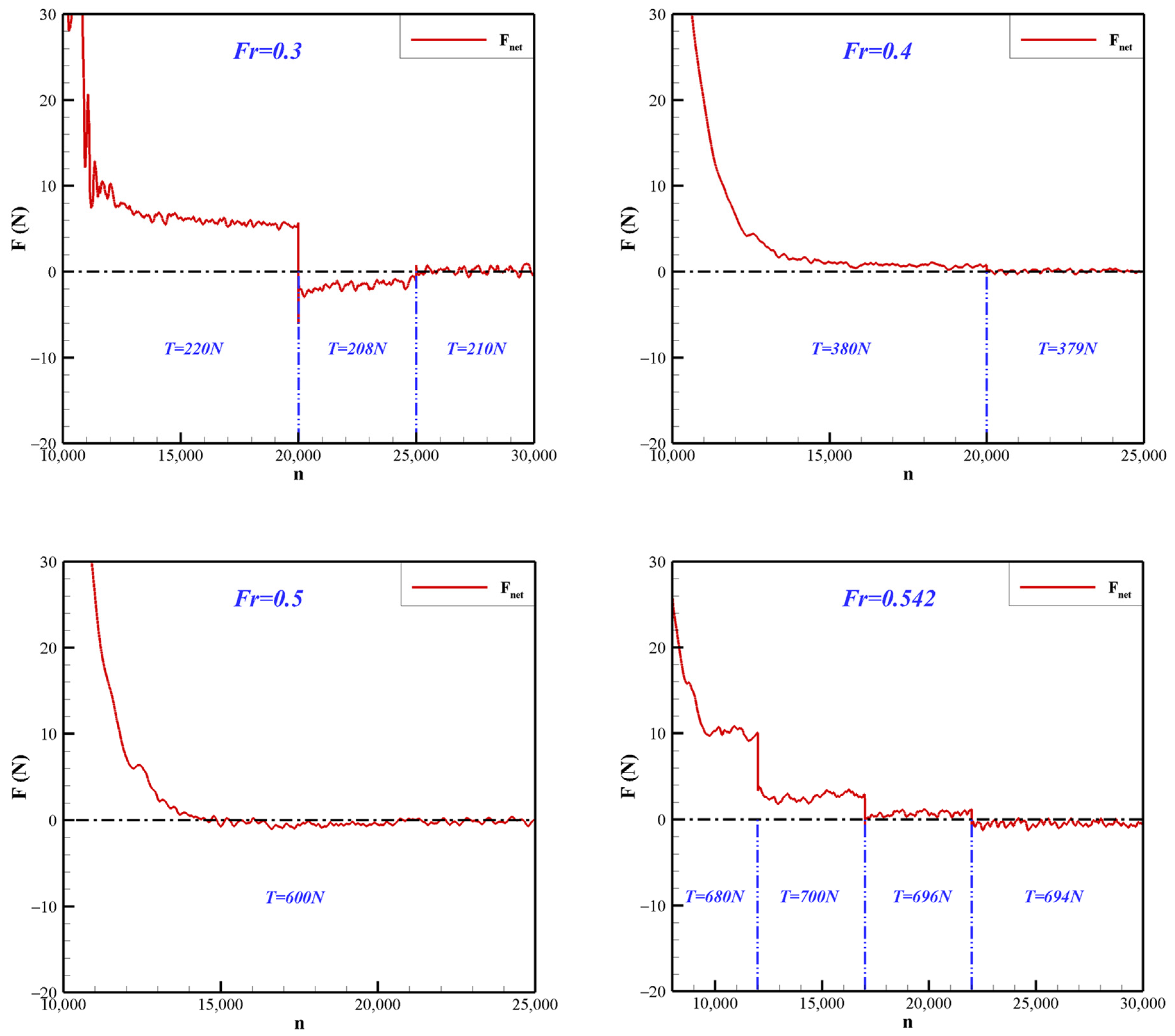To simplify the geometry as much as possible, the impeller and guide vane blades are removed from the body force model, as shown in Figure 6. The initial value of the axial body-force is set equal to the axial force acting on the impeller and the guide vanes computed from the MRF model. Then, for a self-propelled ship, this value has to be adjusted repeatedly to achieve resistance/thrust balance. The self-propulsion is calculated at Fr = 0.3, 0.4, 0.5, 0.542. When the net force of waterjet-propelled ship converges to zero (resistance/thrust balance) in the MRF model, the sliding mesh model is triggered. The time step in the sliding mesh method corresponds to 1° rotation of the impeller. The three methods have the same mesh number in hull region, about 7.22 million. As for the waterjet system, the mesh number in body-force model is about 1.49 million, far smaller than 5.28 million in the MRF and sliding mesh models.

3.2.1. Convergence History and Computational Cost

Figure 9 presents the convergence history of the horizontal force with respect to the impeller rotational speed under different Fr number. When the computation with the MRF model converges, the net force F_net of waterjet-propelled ship (including hull, impeller blades, guide vanes, ducting channel, shaft, hub, etc.) is close to zero. Figure 10 shows the convergence history of the net force F_net of waterjet-propelled ship with the body-force model.

The CPUs used in the present CFD simulations are two 32-core AMD processors at 2.50 GHz. The MRF model and body-force model require about 2.35 hours and 1.68 hours of computational time per 1000 iterations, respectively. Compared with the MRF model, the body-force model can reduce the number of grids by about 30%, and save about 28% in computational time.

3.2.2. External Flow Field

Figure 11 shows the wave patterns of the waterjet-propelled ship with the MRF model and body-force model. It can be seen that the wave patterns with the two different models are almost the same, except for a little difference near the nozzle outlet.

Table 4. Hull resistance of the bare hull (BH), MRF model and body-force model (BFM).

Fr	BH RH (N)	MRF RHM (N)	BFM RHB (N)	Relative Error E (= $\frac{{\mathit{R}}_{\mathit{H}\mathit{B}}-{\mathit{R}}_{\mathit{H}\mathit{M}}}{{\mathit{R}}_{\mathit{H}\mathit{M}}}$)
0.300	98.48	107.94	107.26	−0.63%
0.400	172.15	183.13	183.03	−0.05%
0.500	269.00	278.94	277.66	−0.46%
0.542	309.52	316.72	316.52	−0.06%

lists the hull resistance of the bare hull, MRF model and body-force model. It reveals that the self-propelled hull resistances are larger than the bare hull resistances, and that the relative errors of self-propelled hull resistance with the MRF model and body-force model are less than 0.7%.

Figure 12 shows the jet stream with the MRF model and body-force model under Fr = 0.542 (design speed). Ideally, the counteracting torque caused by the guide vanes should be as large as the impeller torque with an opposite direction to cancel out the swirl in the flow induced by the impeller. However, at this design speed, the torques acting on the impeller and guide vanes are −13.11 N·m and 11.06 N·m, respectively. As a result, the jet surface with the MRF model is not smooth in Figure 12. In contrast, the body-force model predicts a smooth jet surface, which is attributed to a swirl-free jet flow of the body-force model.

3.2.3. Internal Ingested Flow of the Control Volume

Figure 13 displays streamlines tracked upstream from the waterjet pump, which intersects with the incoming boundary layer at station 1a. After that, a program is developed using the MATLAB language to obtain the shape and flow variables of the capture area. Figure 14 exhibits the velocity distributions in the capture area with the MRF model and body-force model at Fr = 0.542, showing the accordance of the axial velocity distribution and the geometry of the capture area obtained by the two models. Figure 15 shows the velocity profiles of the boundary layer at waterjet centerline of the bare hull and the waterjet self-propelled ship using the MRF model and body-force model. The axial velocity at the waterjet centerline of the self-propelled ship is larger than that of the bare hull, due to the suction of the waterjet system. The velocity profiles of the boundary layer at the waterjet centerline of the self-propelled ship with the MRF model and body-force model exhibit little difference.

Similar to the effective wake field on a propeller, the effective wake fraction $w$ is calculated to study the effect of the waterjet suction on the hull distorted flow at station 1a:

$$1-w=\frac{{\displaystyle \underset{A_1}{\iint }{U}_{x}dA}}{{\displaystyle \underset{A_1}{\iint }{U}_{0}dA}}$$

(10)

where $U_0$ is the ship velocity, $A_1$ is the capture area, and $U_x$ is the axial velocity of $A_1$.

The momentum velocity coefficient $C_m$ is defined to quantitatively describe the influence of the hull on the ingested flow as follows:

$$C_m=\frac{1}{U_0}\frac{{\displaystyle \underset{A_1}{\iint }{U}_x^{2}dA}}{{\displaystyle \underset{A_1}{\iint }{U}_{x}dA}}$$

(11)

where $A_1$ is the capture area, $U_x$ is the axial velocity of $A_1$, and $U_0$ is the ship velocity.

The effective wake fraction $w$ and momentum velocity coefficient $C_m$ of the capture area with the MRF model and body-force model are summarized in

Table 5. Calculation $(1-w$ ) and $C_m$ of the capture area with the MRF model and body-force model.

Fr	MRF $$\left(1-{\mathit{w}}_{\mathit{M}}\right)$$	BFM $$\left(1-{\mathit{w}}_{\mathit{B}}\right)$$	$$\begin{gathered} (1-\mathit{w})\mathbf{Error} \\ (=\frac{\left(1-{\mathit{w}}_{\mathit{B}}\right)-\left(1-{\mathit{w}}_{\mathit{M}}\right)}{1-{\mathit{w}}_{\mathit{M}}}) \end{gathered}$$	MRF $${\mathit{C}}_{\mathit{m}\mathit{M}}$$	BFM $${\mathit{C}}_{\mathit{m}\mathit{B}}$$	$$\begin{gathered} {\mathit{C}}_{\mathit{m}} \mathbf{Error} \\ (=\frac{{\mathit{C}}_{\mathit{m}\mathit{B}}-{\mathit{C}}_{\mathit{m}\mathit{M}}}{{\mathit{C}}_{\mathit{m}\mathit{M}}}) \end{gathered}$$
0.300	0.8467	0.8465	−0.02%	0.8711	0.8710	−0.01%
0.400	0.8521	0.8511	−0.12%	0.8768	0.8763	−0.06%
0.500	0.8569	0.8543	−0.30%	0.8817	0.8794	−0.26%
0.542	0.8555	0.8512	−0.50%	0.8808	0.8762	−0.52%

. It shows that the non-uniformity of the capture area with the body-force model is slightly smaller than that with the MRF model. With the increase in speed, the result error between the two models becomes larger, but the relative errors are less than 0.6%.

Figure 16 compares the non-dimensional axial velocity distribution with the MRF model and body-force model at station 3. In general, the velocity distributions with the two models on the inflow plane are similar. The high-speed flow is distributed near the bottom dead center, and the velocity in the lower half disk is higher than that in the upper half disk.

Figure 17 exhibits the non-dimensional axial velocity distribution on the nozzle section with the MRF model and body-force model. The value ${\beta }_{M6}$ is a momentum non-uniformity factor [13], related to the experimental procedure for determining momentum at station 6:

$${\beta }_{M6}=\frac{1}{A_6{\overline{U}}_6^2}{\displaystyle \int U{U}_{x}d{A}_6}$$

(12)

where ${\overline{U}}_6$ is the average velocity of the nozzle section. ${\beta }_{M6}$ is unity for uniform flow, and it deviates from unity as the flow field varies.

Table 6. Results of $NVR$, $Q_J$ and ${\beta }_{M6}$ at station 6 with the MRF model and body-force model (BFM).

Fr	MRF $$\mathit{N}\mathit{V}{\mathit{R}}_{\mathit{M}}$$	BFM $$\mathit{N}\mathit{V}{\mathit{R}}_{\mathit{B}}$$	$$\mathit{N}\mathit{V}\mathit{R}$$ Error	MRF $${\mathit{Q}}_{\mathit{J}\mathit{M}}({\mathbf{m}}^3/\mathbf{s})$$	BFM $${\mathit{Q}}_{\mathit{J}\mathit{B}}({\mathbf{m}}^3/\mathbf{s})$$	$${\mathit{Q}}_{\mathit{J}}$$ Error	MRF $${\mathit{\beta }}_{\mathit{M}6\mathit{M}}$$	BFM $${\mathit{\beta }}_{\mathit{M}6\mathit{B}}$$	$${\mathit{\beta }}_{\mathit{M}6}$$ Error
0.300	1.4823	1.4682	−0.95%	0.0323	0.0322	−0.31%	1.0115	1.0074	−0.41%
0.400	1.4932	1.4831	−0.68%	0.0434	0.0432	−0.46%	1.0114	1.0093	−0.21%
0.500	1.5122	1.4950	−1.14%	0.0549	0.0545	−0.73%	1.0118	1.0082	−0.36%
0.542	1.4973	1.4863	−0.73%	0.0589	0.0587	−0.34%	1.0116	1.0083	−0.33%

lists the results of nozzle velocity ratio NVR ($NVR={\overline{U}}_6/U_0$), flow rate of waterjet $Q_J$ and momentum non-uniformity factor ${\beta }_{M6}$ at station 6 with the MRF model and body-force model. Compared with the MRF model, the momentum non-uniformity factor at station 6 with the body-force model is slightly smaller, due to the simplification of the impeller and guide vanes. At the self-propulsion point, the nozzle velocity ratio and flow rate of waterjet with the body-force model are also slightly smaller. Additionally, the relative errors of the three variables with the two models are less than 1.2%.

Figure 18 presents the detailed flow characteristics at longitudinal section inside the waterjet with the MRF model and body-force model under Fr = 0.542 (design speed). The axial velocity distribution ahead the pump inflow plane and behind the nozzle section with the two models are similar. However, there is a significant difference in the axial velocity distribution between station 3 and station 6, because the impeller and guide vanes are removed in the body-force model.

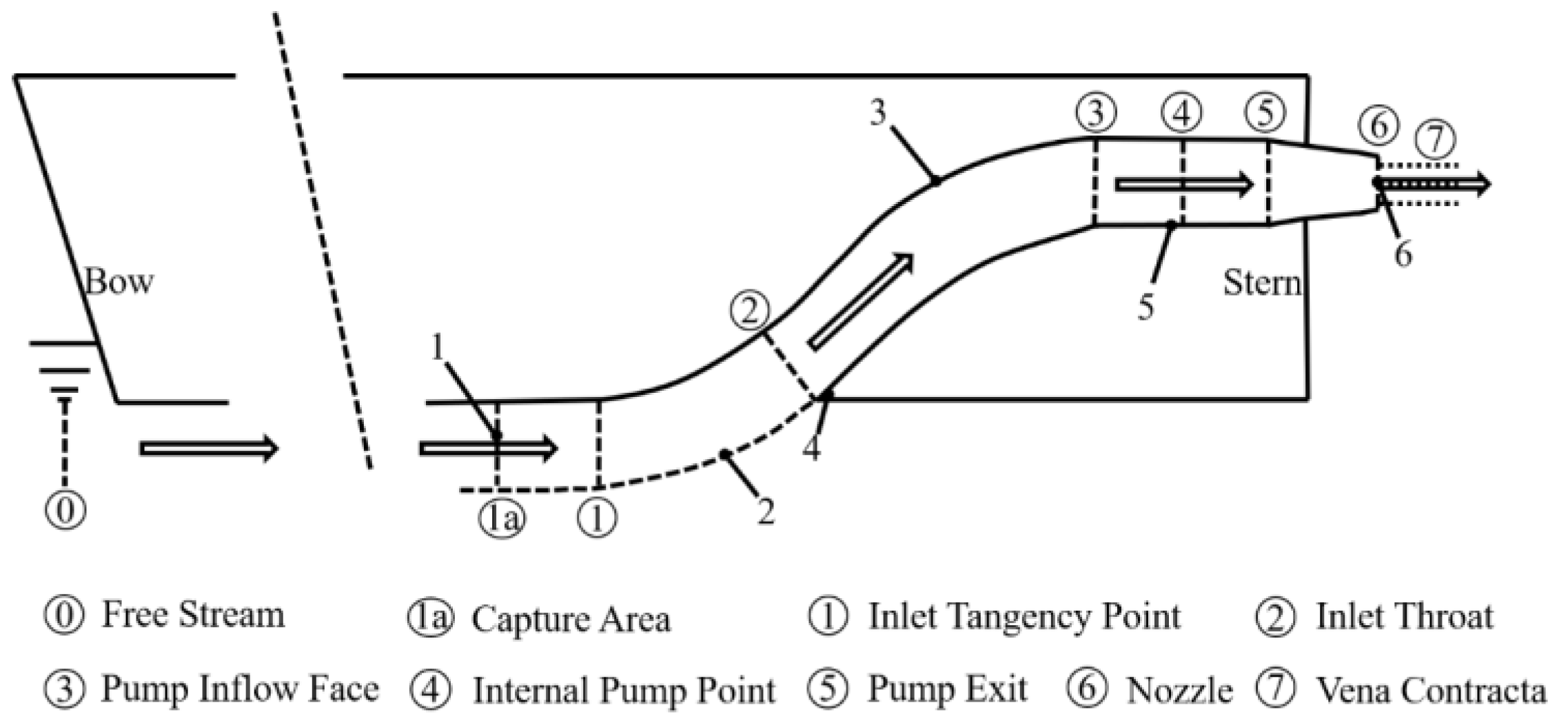
Based on the recommended procedures and guidelines for propulsive performance predictions [4], a control volume is applied to analyze the performance of the waterjet system using the momentum flux method, as shown in Figure 1. Surface 1 is the imaginary capture area. Surface 2 is the imaginary boundary of inlet stream tube, which separates the internal ingested flow of the control volume from the external flow field. Surface 3 is the physical boundary of the waterjet system. Surface 4 is the surface between the stagnation lines and merge lines of the hull and duct. Surface 6 is the nozzle section at station 6.

The horizontal component of the gross thrust vector can be obtained by writing the horizontal momentum flux balance over the control volume:

$$T_{gross}=-{\displaystyle \underset{A_1+A_6}{\iint }\rho u_x(u_k{n}_k)dA}$$

(13)

where $\rho$ is the density of the fluid, $u$ is the velocity vector and $n$ is the unit vector normal to the control surface pointing outward of the control volume [11].

The net thrust is defined as the force vector acting upon the internal material boundary of waterjet system, which acts directly on the hull to balance the resistance. The horizontal component of the net thrust is abbreviated as $T_{net}$ and defined as follows:

$$T_{net}=-{\displaystyle \underset{A_3+A_4}{\iint }{\sigma }_{x}dA}-{\displaystyle \underset{V_{3-5}}{\iiint }\rho F_{px}dV}$$

(14)

where ${\sigma }_x$ is the horizontal component of the surface stresses and $F_{px}$ is the horizontal component of the pump force per unit mass.

For a waterjet-driven hull, the thrust deduction fraction $t$ is not the same as the conventional thrust deduction fraction employed in propeller/hull interaction theory. The thrust deduction fraction relates the resistance of the bare hull to the gross thrust and is defined as follows:

$$1-t=\frac{R_{bh}}{T_{gross}}$$

(15)

Similarly to the conventional thrust deduction fraction employed in propeller/hull interaction theory, the resistance increment fraction $t_r$ based on the bare hull resistance and the net thrust of the waterjet system is defined as follows:

$$1-t_r=\frac{R_{bh}}{T_{net}}$$

(16)

Usually, at the self-propulsion point, the net thrust of waterjet system is equal to the resistance of the self-propelled hull. Therefore, the resistance increment fraction $t_r$ reflects the change in the resistance of the waterjet-propelled hull compared to the bare hull resistance.

In order to relate the net thrust to the gross thrust, the jet system thrust deduction fraction $t_j$ is defined as follows (Eslamdoost, 2014):

$$1-t_j=\frac{T_{net}}{T_{gross}}$$

(17)

Thus, the relationship among the thrust deduction fraction $t$, resistance increment fraction $t_r$ and jet system thrust deduction fraction $t_j$ is

$$1-t=(1-t_r)(1-t_j)$$

(18)

Table 7. Results of $1-t_r$, $1-t_j$ and $1-t$ with the MRF model and body-force model (BFM).

Fr	MRF $1-{\mathit{t}}_{\mathit{r}}$	BFM $1-{\mathit{t}}_{\mathit{r}}$	$1-{\mathit{t}}_{\mathit{r}}$ Error	MRF $1-{\mathit{t}}_{\mathit{j}}$	BFM $1-{\mathit{t}}_{\mathit{j}}$	$1-{\mathit{t}}_{\mathit{j}}$ Error	MRF $1-\mathit{t}$	BFM $1-\mathit{t}$	$1-\mathit{t}$ Error
0.300	0.914	0.917	0.33%	1.111	1.119	0.72%	1.016	1.027	1.08%
0.400	0.946	0.941	0.53%	1.034	1.053	1.84%	0.978	0.991	1.33%
0.500	0.961	0.969	0.87%	0.990	0.998	0.81%	0.951	0.967	1.68%
0.542	0.983	0.980	−0.31%	0.978	0.979	0.10%	0.962	0.959	−0.31%

shows the results of $1-t_r$, $1-t_j$ and $1-t$ with the MRF model and body-force model. With the increase in speed, the resistance increment fraction $t_r$ decreases, and the jet system thrust deduction fraction $t_j$ increases, which is similar to the results for Fr < 0.55 by Guo et al. [32]. Additionally, the relative errors of $1-t_r$, $1-t_j$ and $1-t$ between the two models are less than 1.9%.

3.2.4. Transient Sliding Mesh Model

Taking the results of the MRF model as the initial condition, the sliding mesh model is applied to simulate the transient flow under Fr = 0.542 (design speed). The time step corresponds to 1° rotation of the impeller. Figure 19 exhibits the net force of the waterjet-propelled ship and volume flow rate at station 6 with the MRF model, body-force model and sliding mesh model. In the sliding mesh model, the net force of the waterjet-propelled ship fluctuates within a small range, and the mean value is zero (resistance/thrust balance). The volume flow rate with the sliding mesh model is oscillating within the range of ± 0.42%. However, the net force and volume flow rate computed with the MRF and body-force models are almost constant at the self-propulsion point. This indicates that the sliding mesh model is capable of capturing the unsteady periodic characteristics of the actual flow, while the MRF and body-force models cannot.

Figure 20 shows the non-dimensional axial velocity distribution at station 3 and 6 at a certain time with the sliding mesh model, which shows more uneven axial velocity distribution in the upper half disk of station 3, compared with the MRF and body-force models.

Table 8. Results of $NVR$, $Q_J$ and ${\beta }_{M6}$ at station 6 with the MRF model, body-force model (BFM) and sliding mesh model (SMM).

	MRF	BFM	SMM
$NVR$	1.4973	1.4863	1.5234
$Q_J$ (m3/s)	0.0589	0.0587	0.0599
${\beta }_{M6}$	1.0116	1.0083	1.0094

lists the results of nozzle velocity ratio NVR ($NVR={\overline{U}}_6/U_0$), flow rate of waterjet $Q_J$ and momentum non-uniformity factor ${\beta }_{M6}$ at station 6 with the MRF model, body-force model and sliding mesh model. The nozzle velocity ratio and flow rate of waterjet with the sliding mesh model are larger than those of the MRF and body-force models. Compared with the body-force model, the momentum non-uniformity factor at station 6 with the sliding mesh model is slightly greater.

4. Conclusions

In the current research, numerical simulations and analysis of self-propulsion for a waterjet-propelled ship model are conducted. The grid independence study is performed for the bare hull to define the computational mesh in hull region. For the self-propulsion of the waterjet-propelled ship model, the computational cost, external flow filed, and internal ingested flow field of the control volume with the MRF model and body-force model are compared. The transient sliding mesh model is triggered when the net force of waterjet-propelled ship converges to zero (resistance/thrust balance) with the steady MRF model simulation at Fr = 0.542 (design speed). The main conclusions are presented below:

(1)

Compared with the MRF model, the body-force model can reduce the number of grids by about 30%, and save about 28% in the computational time. In addition, the wave pattern and self-propelled hull resistance obtained by the body-force model agree well with that of MRF model, indicating that the body-force model is economical and efficient when the primary concerns are related to the external flow field.

(2)

The velocity profiles of the boundary layer at the waterjet centerline of the capture area with the MRF model and body-force model show little difference, and the non-uniformity of the capture area with the body-force model is slightly smaller than that with the MRF model.

(3)

As for the nozzle section, the momentum non-uniformity factor with the body-force model is slightly smaller compared with the MRF model. At the self-propulsion point, the nozzle velocity ratio ($NVR$ ) and flow rate of waterjet with the body-force model are also slightly smaller.

(4)

As the speed grows, the resistance increment fraction $t_r$ decreases, while the jet system thrust deduction fraction $t_j$ increases. Additionally, the relative errors of $1-t_r$, $1-t_j$ and $1-t$ between the MRF model and body-force model are less than 1.9%.

(5)

The volume flow rate and the net force of waterjet-propelled ship with the transient sliding mesh model fluctuate in a small range, while the values with the steady MRF and body-force models remain constant at self-propulsion point. Additionally, the axial velocity distribution in the upper half disk of station 3 with the sliding mesh model is more uneven than that with the MRF and body-force models. The nozzle velocity ratio, flow rate of waterjet and momentum non-uniformity factor at station 6 with the sliding mesh model are greater, compared with the body-force model.

References

1. ITTC. Report of the waterjets group, appendix A. In Proceedings of the 21st International Towing Tank Conference (ITTC), Trondheim, Norway, 15–21 September 1996. [Google Scholar]
2. ITTC. The specialist committee on waterjets final report and recommendations to the 22nd ITTC. In Proceedings of the 22nd International Towing Tank Conference (ITTC), Seoul, Korea & Shanghai, China, 5–11 September 1999. [Google Scholar]
3. ITTC. The Specialist Committee on Validation of Waterjet Test Procedures. In Proceedings of the 23rd International Towing Tank Conference (ITTC), Venice, Italy, 8–14 September 2002; Volume II, pp. 387–415. [Google Scholar]
4. ITTC. Report of the specialist committee on validation of waterjet test procedures. In Proceedings of the 24th International Towing Tank Conference (ITTC), Edinburgh, UK, 4–10 September 2005. [Google Scholar]
5. ITTC. The specialist committee on waterjets: Final report and recommendations to the 25th ITTC. In Proceedings of the 25th International Towing tank Conference (ITTC), Fukuoka, Japan, 14–20 September 2008. [Google Scholar]
6. ITTC. The propulsion committee: Final report and recommendations to the 26th ITTC. In Proceedings of the 26th International Towing Tank Conference (ITTC), Rio de Janeiro, Brazil, 28 August–3 September 2011. [Google Scholar]
7. ITTC. The propulsion committee: Final report and recommendations to the 27th ITTC. In Proceedings of the 27th International Towing Tank Conference (ITTC), Copenhagen, Denmark, 31 August–5 September 2014. [Google Scholar]
8. ITTC. The propulsion committee: Final report and recommendations to the 28th ITTC. In Proceedings of the 28th International Towing Tank Conference (ITTC), Wuxi, China, 17–23 September 2017. [Google Scholar]
9. ITTC. The ocean engineering committee: Final report and recommendations to the 29th ITTC. In Proceedings of the International Towing Tank Conference (ITTC), Paris, France, 6 September–10 December 2021. [Google Scholar]
10. Coop, H.G. Investigation of Hull-Waterjet Interaction Effects. Ph.D. Thesis, Department of Mechanical Engineering, University of Canterbury, Christchurch, New Zealand, 1995. [Google Scholar]
11. Terwisga, T.V. Waterjet-Hull Interaction. Ph.D. Thesis, Delft Technical University, Delft, The Netherlands, 1996. [Google Scholar]
12. Bulten, N.W.H. Numerical Analysis of a Waterjet Propulsion System. Ph.D. Thesis, Eindhoven University of Technology, Eindhoven, The Netherlands, 2006. [Google Scholar]
13. Delaney, K.; Donnelly, M.; Ebert, M.; Fry, D. Use of RANS for waterjet analysis of a high-speed Sealift concept vessel. In Proceedings of the First International Symposium on Marine Propulsors (Smp’09), Trondheim, Norway, 22–24 June 2009. [Google Scholar]
14. Kandasamy, M.; Ooi, S.K.; Carrica, P.; Stern, F. Integral force/moment waterjet model for CFD simulations. J. Fluids Eng. 2021, 132, 1–9. [Google Scholar] [CrossRef]
15. Takai, T.; Kandasamy, M.; Stern, F. Verification and validation study of URANS simulations for an axial waterjet propelled large high-speed ship. J. Mar. Sci. Technol. 2011, 16, 434–447. [Google Scholar] [CrossRef]
16. Eslamdoost, A.; Larsson, L.; Bensow, R. A pressure jump method for modelling waterjet/hull interaction. Ocean Eng. 2014, 88, 120–130. [Google Scholar] [CrossRef]
17. Eslamdoost, A. The Hydrodynamics of Waterjet/Hull Interaction. Ph.D. Thesis, Shipping and Marine Technology, Chalmers University of Technology, Gothenburg, Sweden, 2014. [Google Scholar]
18. Eslamdoost, A.; Larsson, L.; Bensow, R. Net and gross thrust in waterjet propulsion. J. Ship Res. 2016, 60, 78–91. [Google Scholar] [CrossRef]
19. Eslamdoost, A.; Larsson, L.; Bensow, R. Analysis of the thrust deduction in waterjet propulsion—The Froude number dependence. Ocean Eng. 2018, 152, 100–112. [Google Scholar] [CrossRef]
20. Gong, J.; Guo, C.Y.; Wang, C.; Wu, T.C.; Song, K.W. Analysis of waterjet-hull interaction and its impact on the propulsion performance of a four-waterjet-propelled ship. Ocean Eng. 2019, 180, 211–222. [Google Scholar] [CrossRef]
21. Liu, C.; Chen, H.; Ma, Z. Influence of non-uniform inflow on unsteady internal flow characteristics of waterjet pump. Mod. Phys. Lett. B 2022, 36, 2150576. [Google Scholar] [CrossRef]
22. Guo, J.; Chen, Z.; Dai, Y. Numerical study on self-propulsion of a waterjet propelled trimaran. Ocean Eng. 2020, 195, 106655. [Google Scholar] [CrossRef]
23. Ji, X.-Q.; Dong, X.-Q.; Yang, C.-J. Attenuation of the tip-clearance flow in a pump-jet propulsor by thickening and raking the tips of rotor blades: A Numerical Study. Appl. Ocean Res. 2021, 113, 102723. [Google Scholar] [CrossRef]
24. Jiang, J.; Ding, J. The hull-waterjet interaction of a planing trimaran. Ocean Eng. 2021, 221, 108534. [Google Scholar] [CrossRef]
25. Jiang, J.; Ding, J.; Gong, J.; Li, L. Effect of hull displacement on hydro- & aerodynamics of a planing trimaran. Appl. Ocean Res. 2022, 120, 103050. [Google Scholar]
26. Jiang, J.; Ding, J.; Chang, R.; Luo, H.; Gong, J. Respective effect of waterjet suction and jet action on hull resistance. Ocean Eng. 2022, 255, 111398. [Google Scholar] [CrossRef]
27. Gong, J.; Liu, J.; Dai, Y.; Guo, C.; Wu, T. Dynamics of stabilizer fins on the waterjet-propelled ship. Ocean Eng. 2021, 222, 108595. [Google Scholar] [CrossRef]
28. Knight, B.G.; Maki, K.J. A semi-empirical multi-degree of freedom body force propeller model. Ocean Eng. 2019, 178, 270–282. [Google Scholar] [CrossRef]
29. Jin, Y.; Duffy, J.; Chai, S.; Magee, A.R. DTMB 5415M dynamic manoeuvres with URANS computation using body-force and discretised propeller models. Ocean Eng. 2019, 182, 305–317. [Google Scholar] [CrossRef]
30. Feng, D.; Yu, J.; He, R.; Zhang, Z.; Wang, Z. Free running computations of KCS with different propulsion models. Ocean Eng. 2020, 214, 107563. [Google Scholar] [CrossRef]
31. Feng, D.; Yu, J.; He, R.; Zhang, Z.; Wang, Z. Improved body force propulsion model for ship propeller simulation. Appl. Ocean Res. 2020, 104, 102328. [Google Scholar] [CrossRef]
32. Guo, C.; Wang, X.; Wang, C.; Zhao, Q.; Zhang, H. Research on calculation methods of ship model self-propulsion prediction. Ocean Eng. 2020, 203, 107232. [Google Scholar] [CrossRef]
33. Yu, J.; Yao, C.; Liu, L.; Zhang, Z.; Feng, D. Assessment of full-scale KCS free running simulation with body-force models. Ocean Eng. 2021, 237, 109570. [Google Scholar] [CrossRef]
34. Eslamdoost, A.; Vikström, M. A Body-Force Model for Waterjet Pump Simulation. Appl. Ocean Res. 2019, 90, 101832. [Google Scholar] [CrossRef]
35. Menter, F.R. Two-equation eddy-viscosity turbulence models for engineering applications. AIAA J. 1994, 32, 1598–1605. [Google Scholar] [CrossRef] [Green Version]
36. Hirt, C.W.; Nichols, B.D. Volume of fluid (VOF) method for the dynamics of free boundaries. J. Comput. Phys. 1981, 39, 201–225. [Google Scholar] [CrossRef]
37. Snyder, D.; Koutsavdis, E.; Anttonen, J. Transonic Store Separation Using Unstructured CFD with Dynamic Meshing. In Proceedings of the 33rd AIAA Fluid Dynamics Conference and Exhibit, Orlando, FL, USA, 23–26 June 2003. [Google Scholar]
38. Demirdzic, I.; Peric, M. Space Conservation Law in Finite Volume Calculations of Fluid Flow. Int. J. Numer. Methods Fluids 1988, 8, 1037–1050. [Google Scholar] [CrossRef]
39. Eça, L.; Hoekstra, M. A procedure for the estimation of the numerical uncertainty of CFD calculations based on grid refinement studies. J. Comput. Phys. 2014, 262, 104–130. [Google Scholar] [CrossRef]
Figure 1. Definition of the momentum flux method reference stations.
Applsci 12 07148 g001
Figure 2. Hull and waterjet geometry.
Applsci 12 07148 g002
Figure 3. Computational domain and boundary conditions.
Applsci 12 07148 g003
Figure 4. Computational grid system of the waterjet-propelled ship model.
Applsci 12 07148 g004
Figure 5. The mesh of waterjet system.
Applsci 12 07148 g005
Figure 6. Geometry used with body-force model.
Applsci 12 07148 g006
Figure 7. Convergence of the total resistance.
Applsci 12 07148 g007
Figure 8. Numerical results (CFD) and experimental data (EFD) of bare hull resistance.
Applsci 12 07148 g008
Figure 9. Convergence history of the net force Fnet of waterjet-propelled ship with the MRF model.
Applsci 12 07148 g009
Figure 10. Convergence history of the net force Fnet of waterjet-propelled ship with the body-force model.
Applsci 12 07148 g010
Figure 11. Wave patterns of the waterjet-propelled ship with the MRF model and body-force model (BFM). (a) Fr = 0.3; (b) Fr = 0.4; (c) Fr = 0.5; (d) Fr = 0.542.
Applsci 12 07148 g011
Figure 12. Jet stream with the MRF model and body-force model (BFM).
Applsci 12 07148 g012
Figure 13. Waterjet streamlines calculated by RANS intersecting station 1a boundary layer.
Applsci 12 07148 g013
Figure 14. Velocity distributions in the capture area with the MRF model and body-force model (BFM).
Applsci 12 07148 g014
Figure 15. Velocity profiles of boundary layer at waterjet centerline of the bare hull (BH), MRF model and body-force model (BFM). ζ is the vertical distance from ship bottom plating.
Applsci 12 07148 g015
Figure 16. Comparison of non-dimensional axial velocity distribution of the MRF model and body-force model (BFM) at station 3. (a) Fr = 0.3; (b) Fr = 0.4; (c) Fr = 0.5; (d) Fr = 0.542.
Applsci 12 07148 g016
Figure 17. Comparison of non-dimensional axial velocity distribution of the MRF model and body-force model (BFM) at station 6. (a) Fr = 0.3; (b) Fr = 0.4; (c) Fr = 0.5; (d) Fr = 0.542.
Applsci 12 07148 g017
Figure 18. Non-dimensional axial velocity at longitudinal section inside the waterjet with the MRF model and body-force model (BFM).
Applsci 12 07148 g018
Figure 19. Net force of waterjet-propelled ship and volume flow rate at station 6 (VFR-6) with three different models.
Applsci 12 07148 g019
Figure 20. Non-dimensional axial velocity distribution at station 3 and 6 with three different models.
Applsci 12 07148 g020