
An Attempt to Study Foundation Anchoring Conditions in Sedimentary Estuaries Using Integrated Methods

Abstract
:1. Introduction
2. Materials
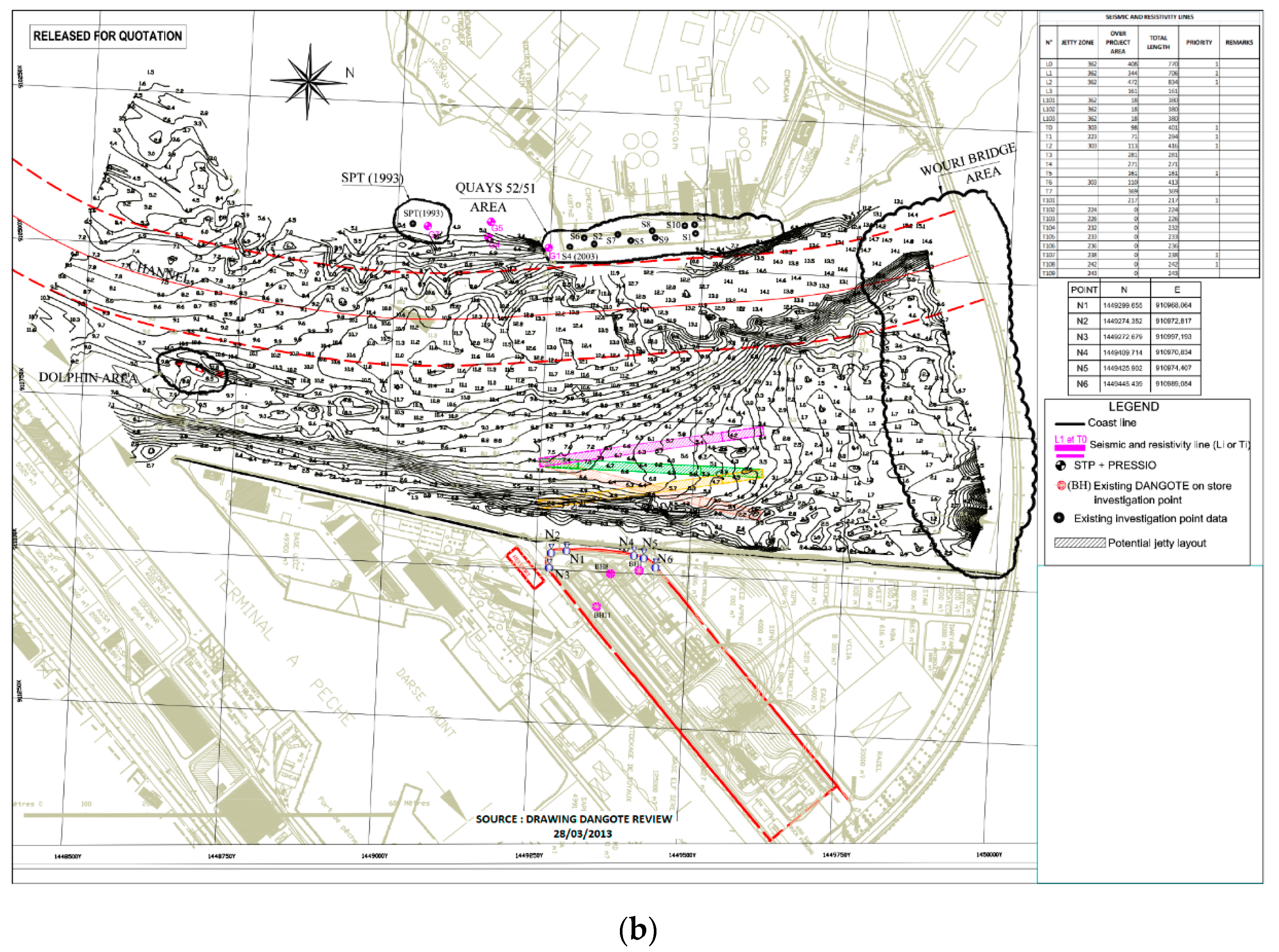
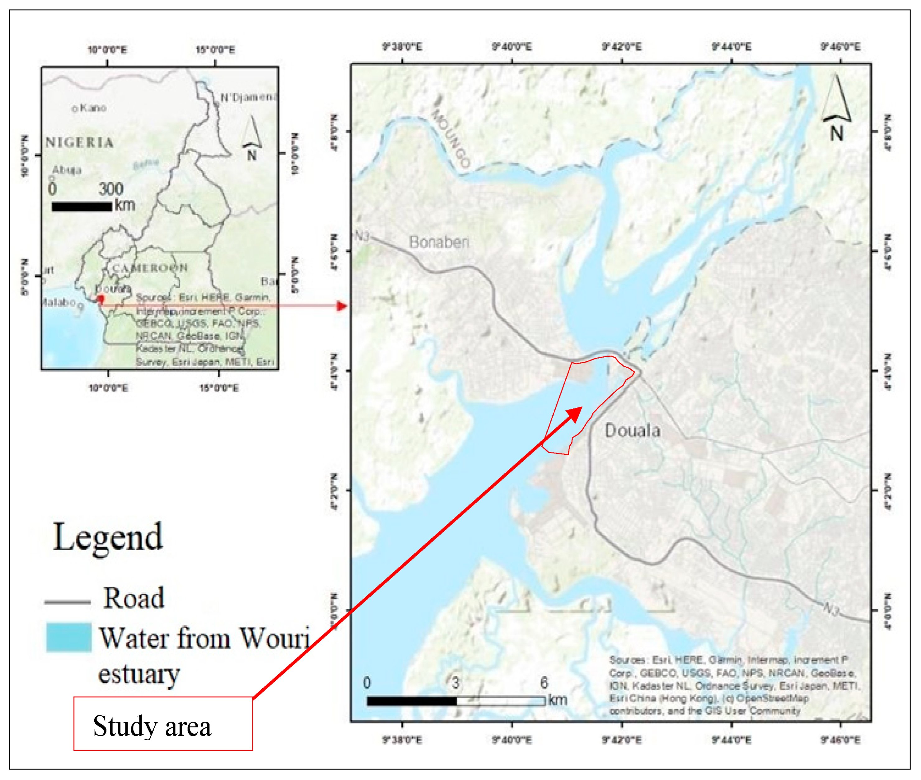
2.1. Study Area Description
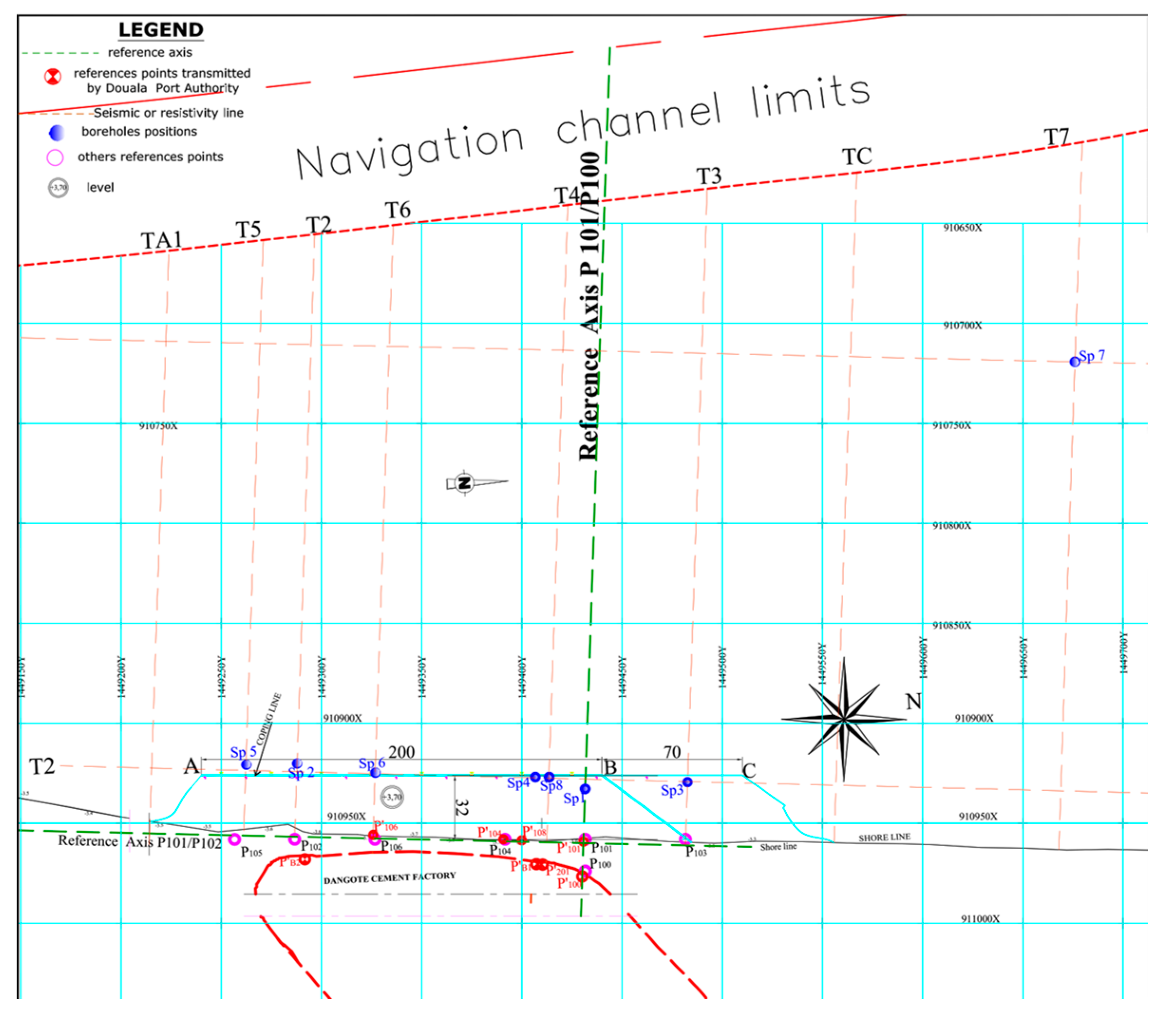
2.2. In Situ Measurements
3. Methods
3.1. Bathymetry and Sides-Can Sonar
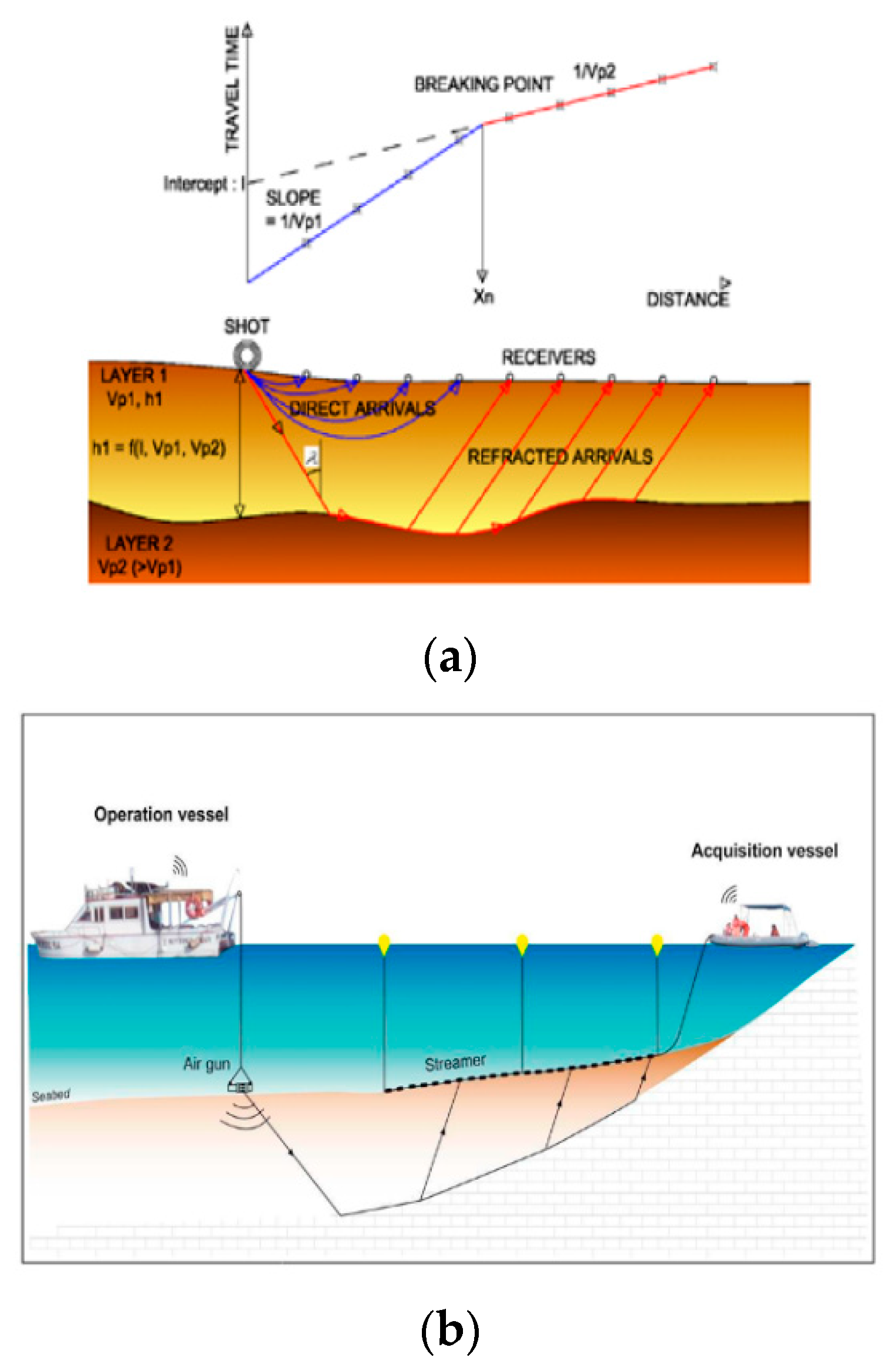
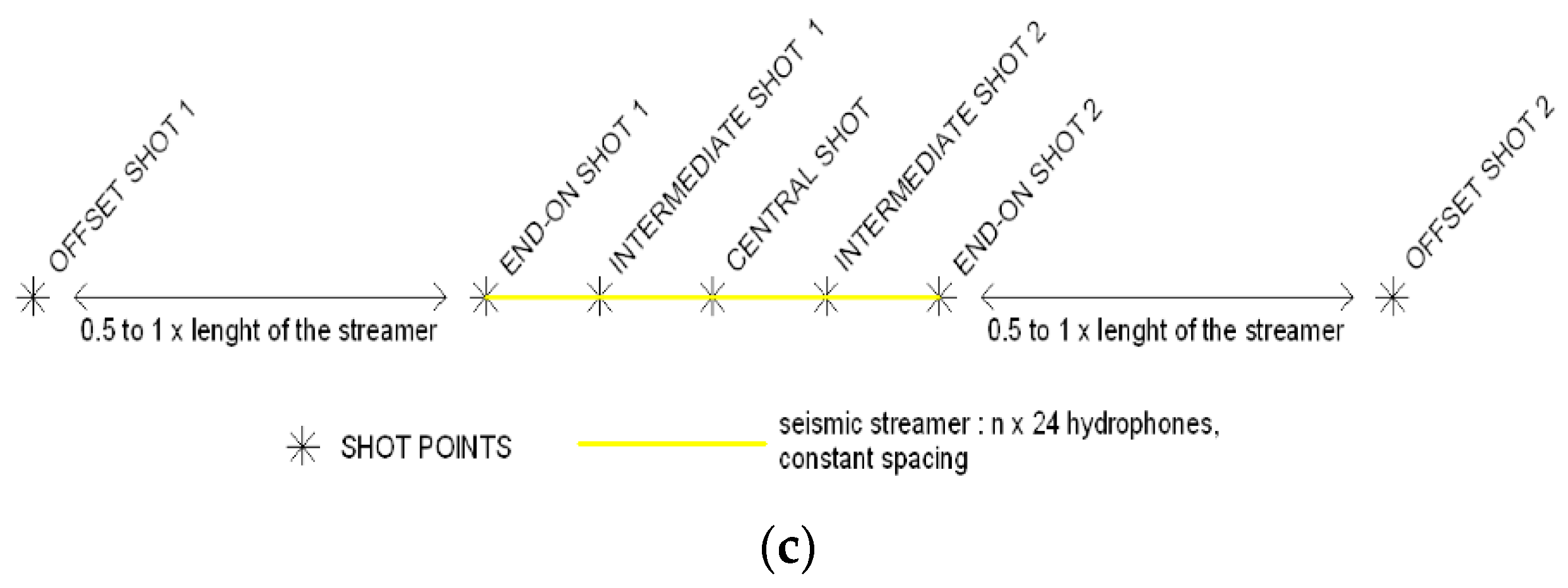
3.2. Seismic Refraction by Streamer
3.3. SPT Type Mechanical Borehole
3.4. Pressuremeter Test
4. Results and Discussion
4.1. Riverbed Topography

4.2. Seismic Sounding and Profiles

4.3. Velocity Calculations
4.4. Time-Distance Curves and Seismic Sections
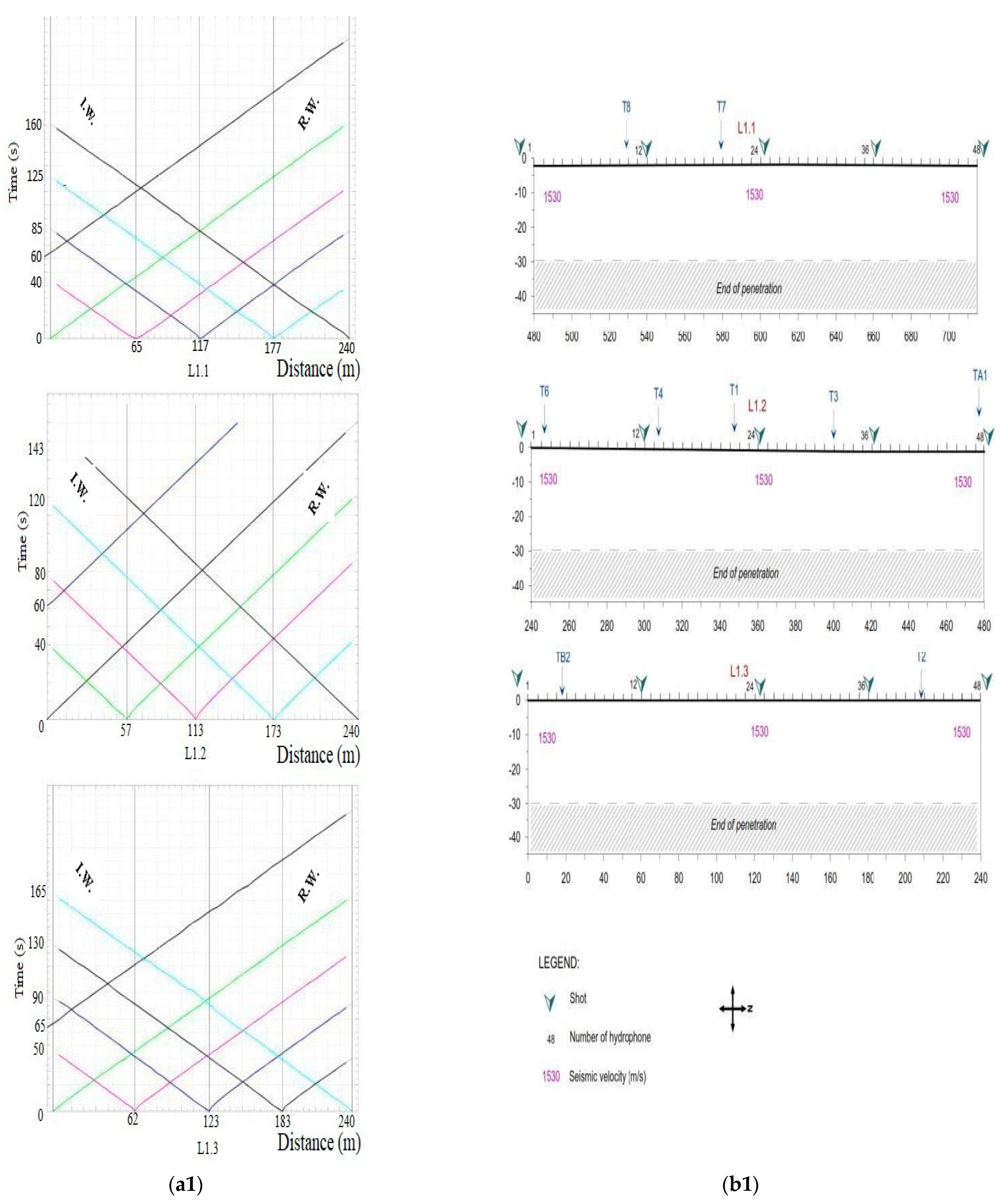
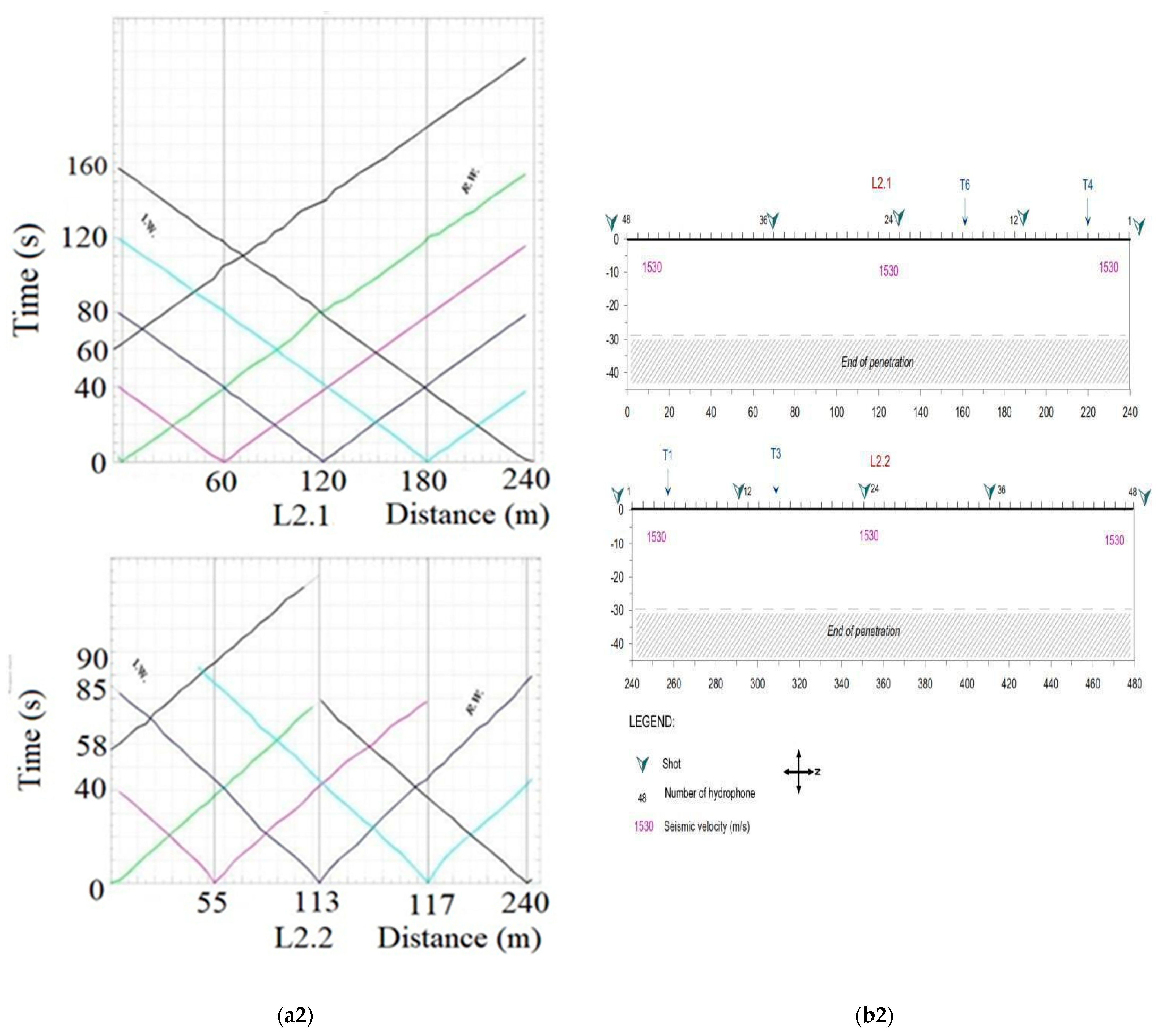


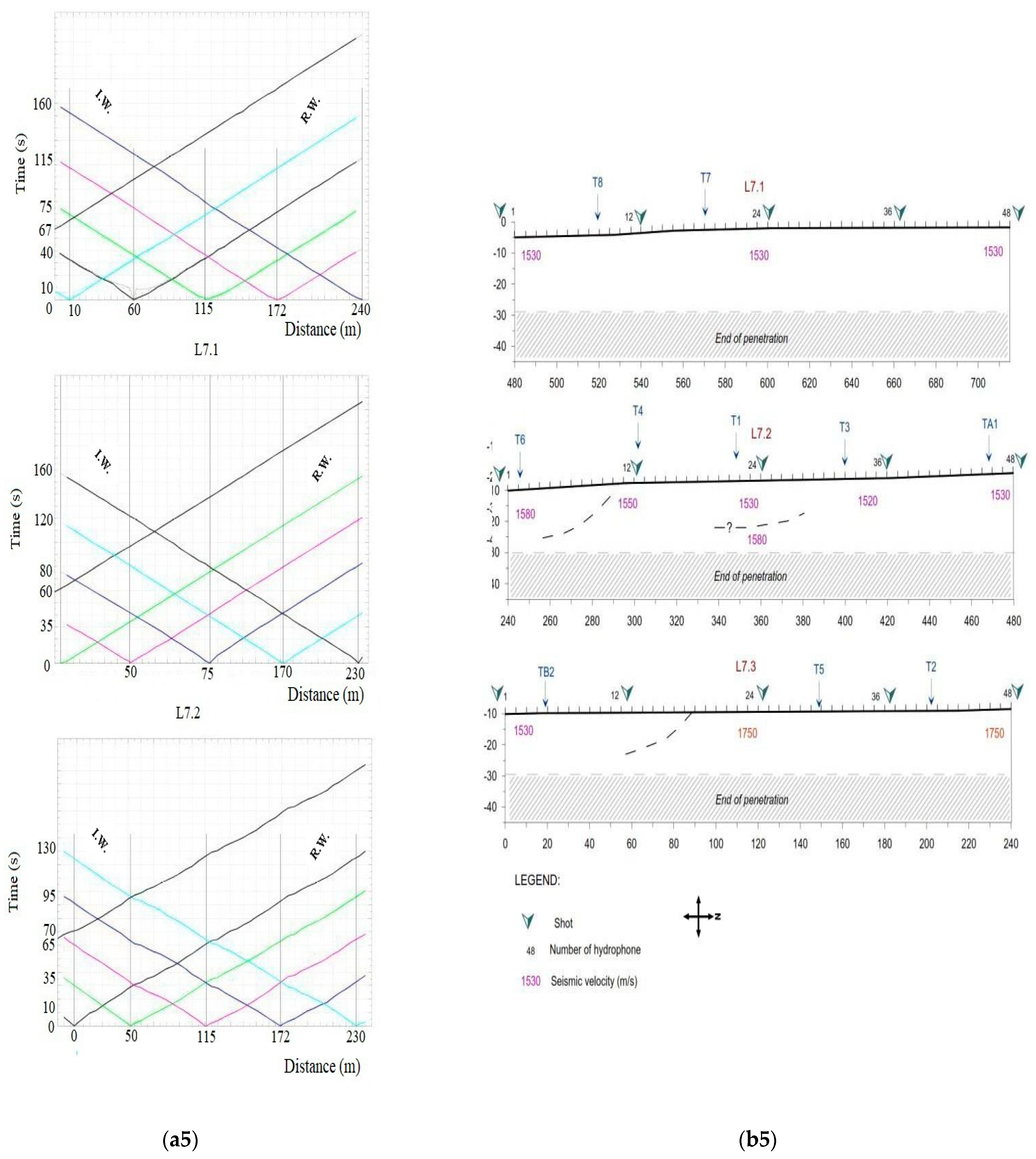

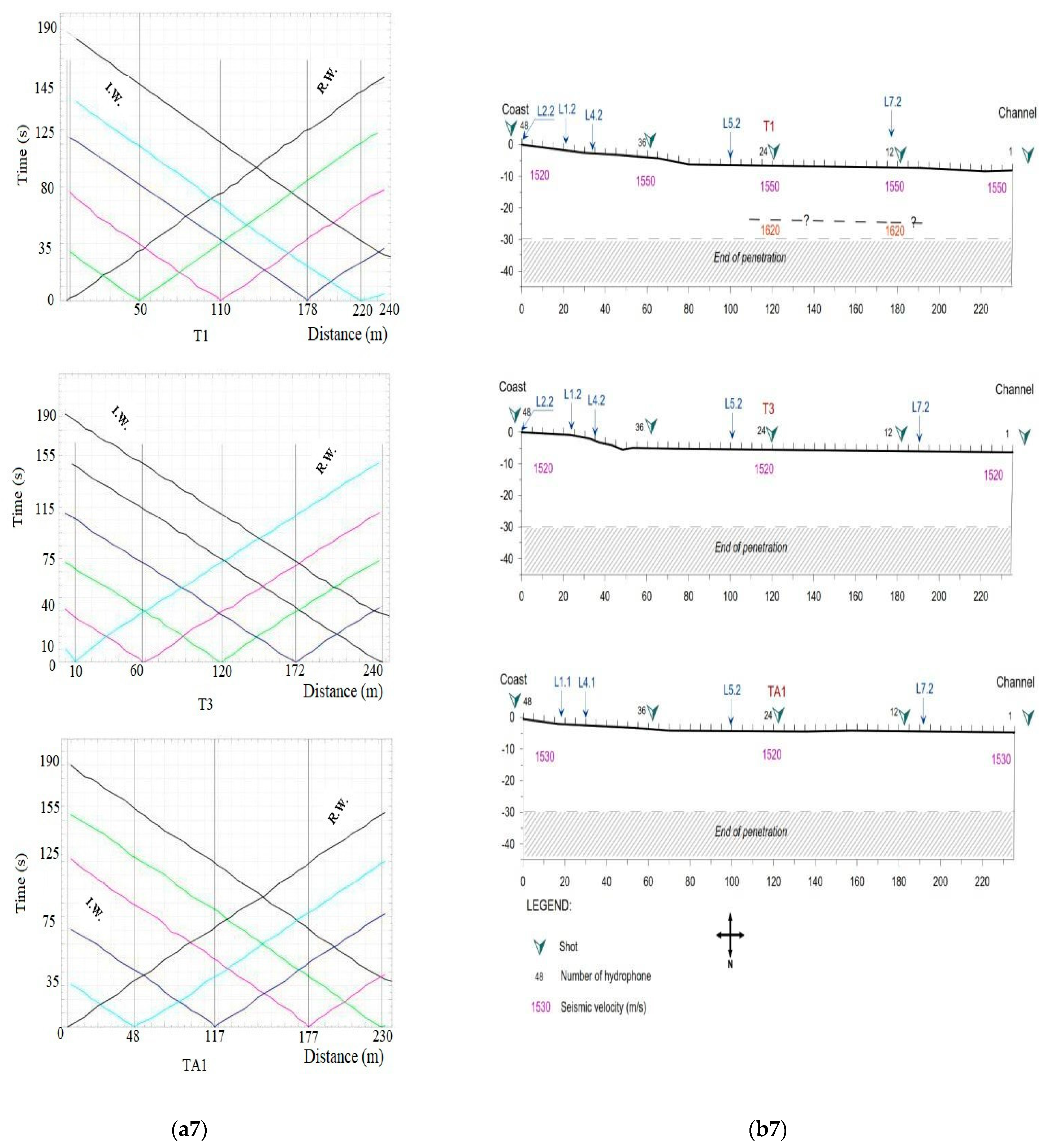
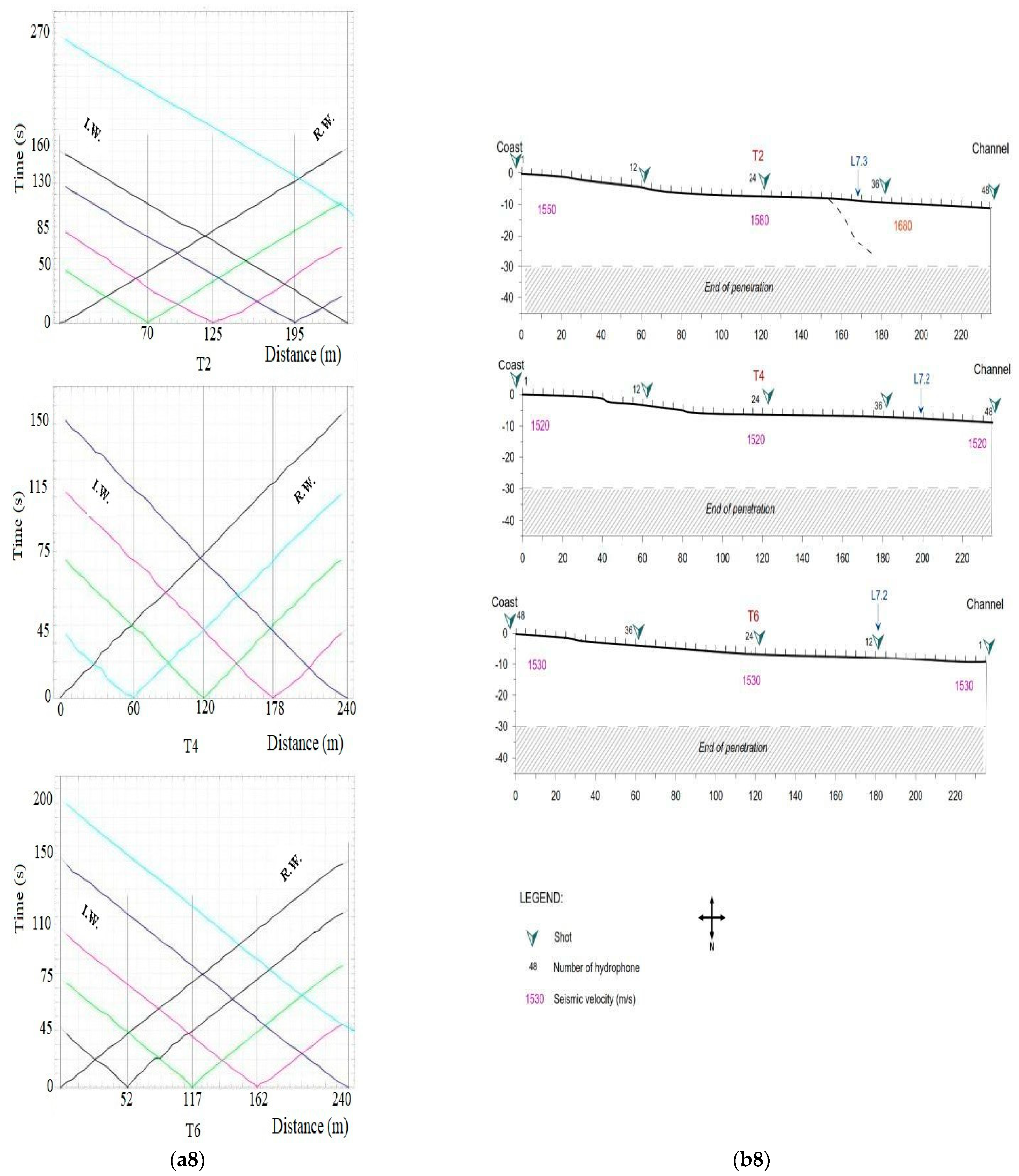
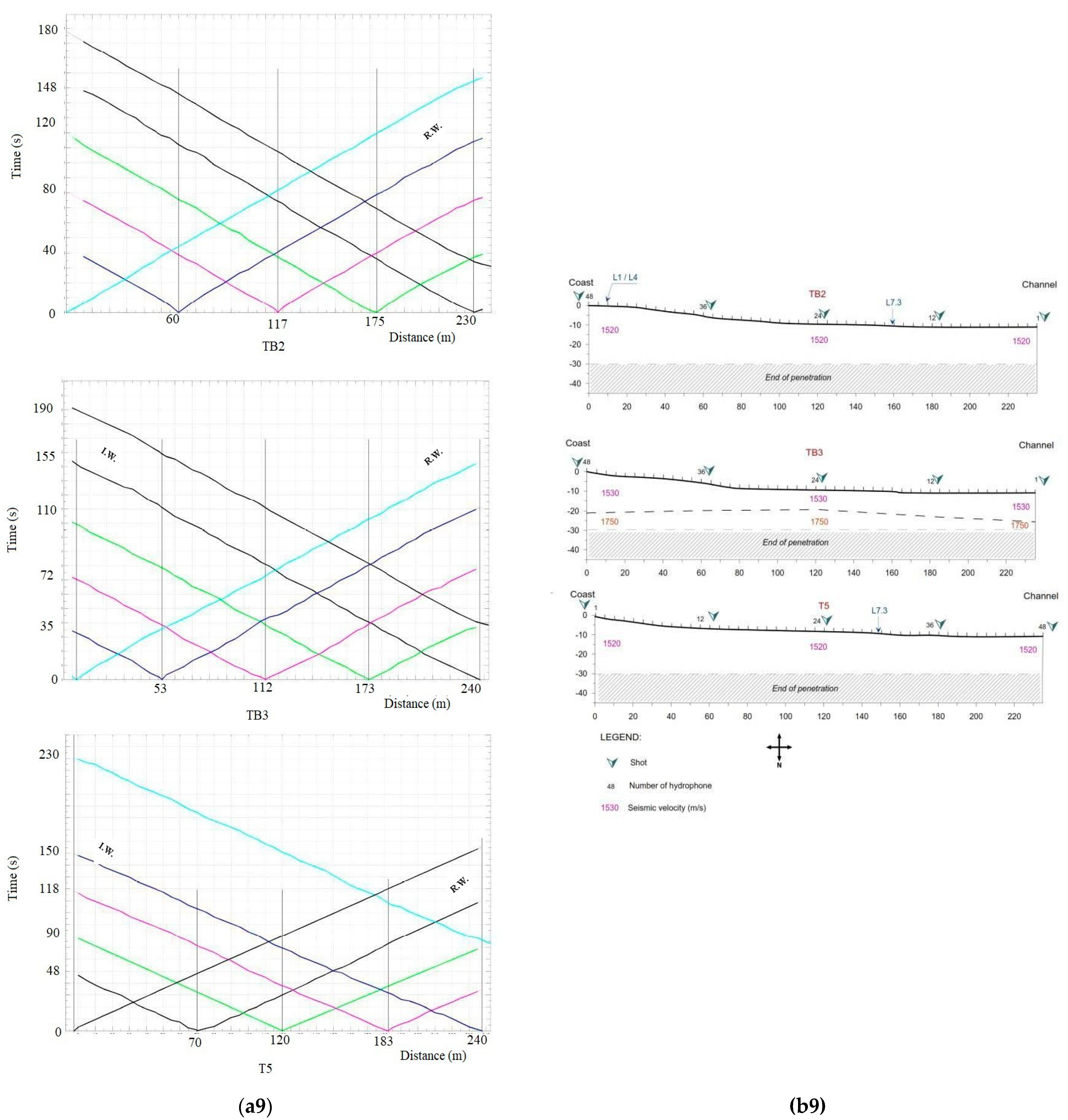
4.5. Determination of Investigation Depths and Seismic Velocities
4.6. Material Identification
4.7. Mechanical Borings
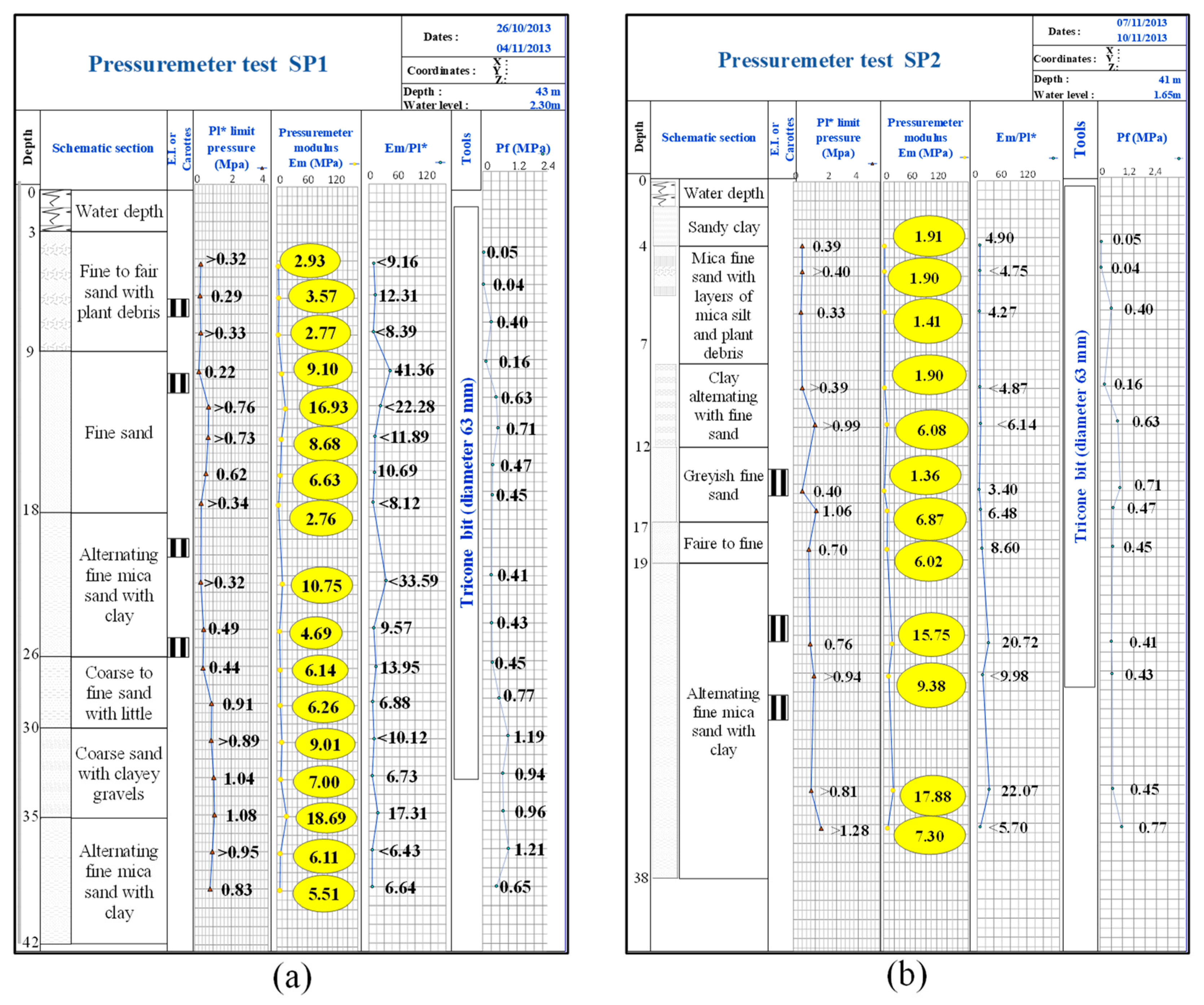
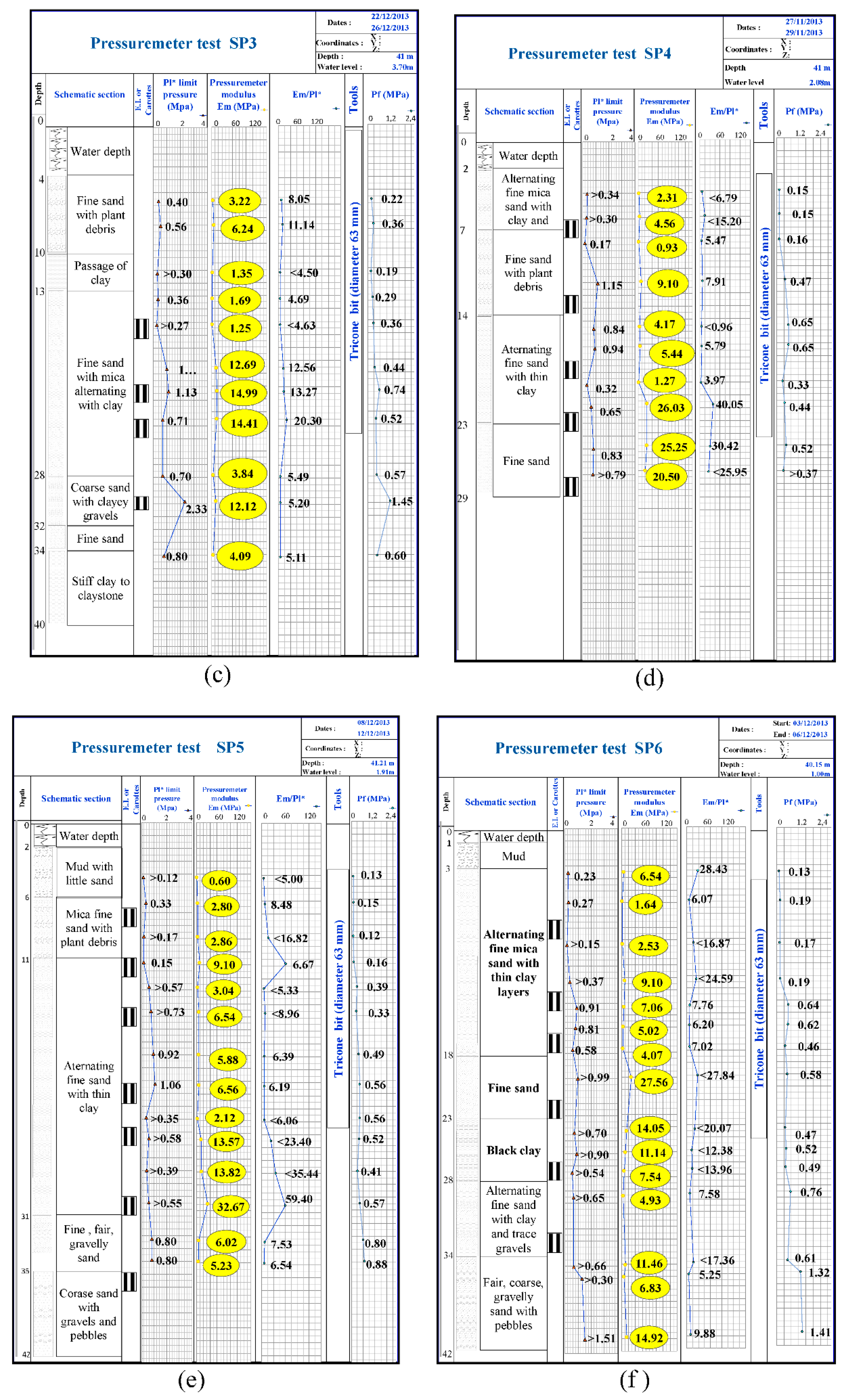
4.8. PMT Results
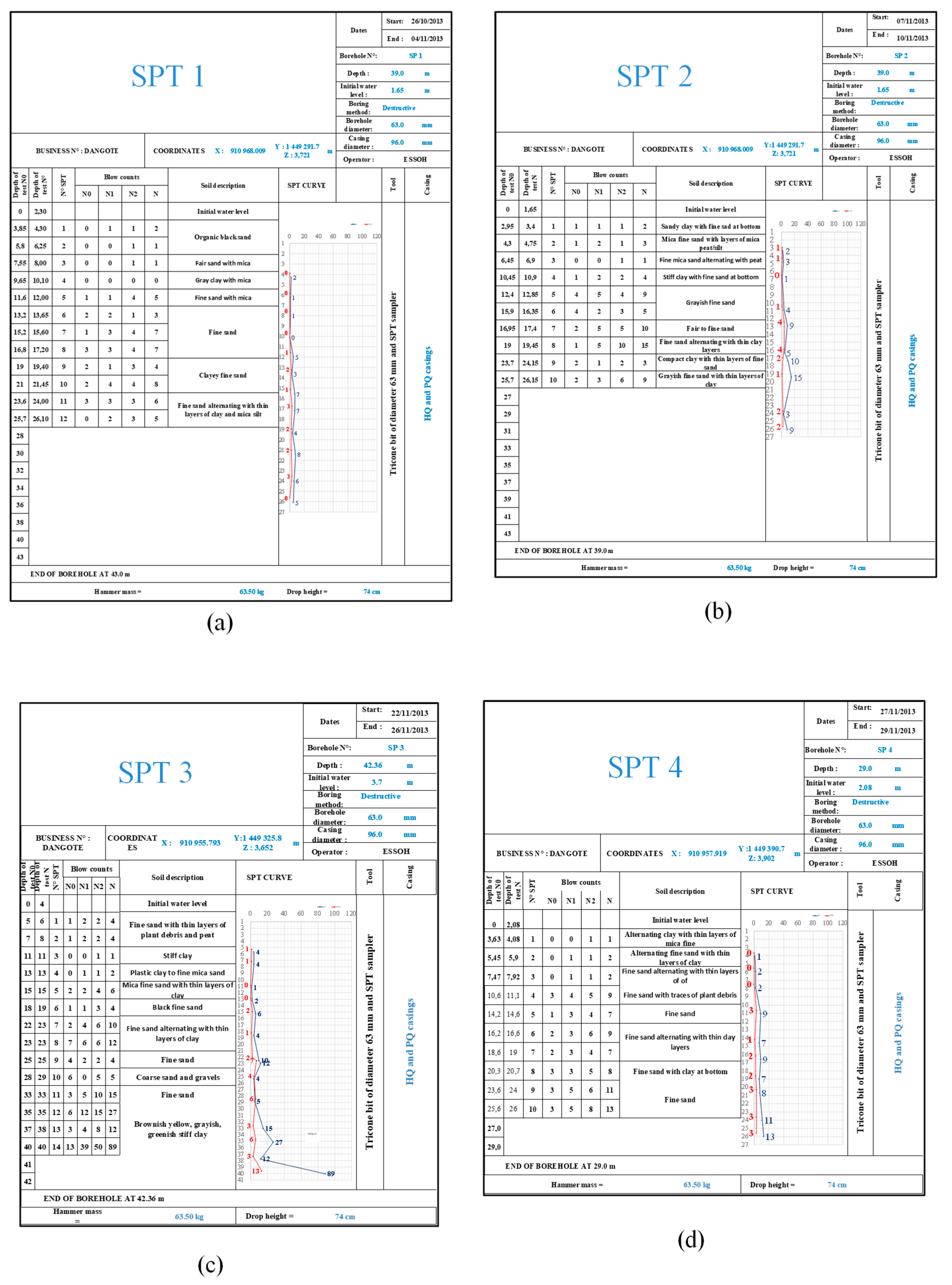
4.9. SPT Results
4.10. Laboratory Tests Results
5. Conclusions
Author Contributions
Funding
Data Availability Statement
Conflicts of Interest
References
- Hartmann, J.; Ocel, J.M.; Wright, W.; Fuchs, P.; Adams, M. I-90 Seaport Portal Tunnel Partial Ceiling Collapse Investigation: Adhesive Anchor Sustained Load Testing Results; Federal Highway Administration, U.S. Department of Transportation: Washington, DC, USA, 2007; p. 82.
- El-Naggar, M. Enhancement of steel sheet-piling quay walls using grouted anchors. J. Soil Sci. Environ. Manag. 2010, 1, 69–76. [Google Scholar] [CrossRef]
- Ribeiro, L.; Santos-Ferreira, A. Vertical Harbour Quay Rehabilitation Using Ground Anchors. Eng. Geol. Soc. Territ. 2014, 6, 279–283. [Google Scholar] [CrossRef]
- The Queensland Government. Anchorage Area Design and Management Guideline Maritime Safety Queensland. 2019. Available online: http://creativecommons.org.licences/by/4.0 (accessed on 12 April 2022).
- Ralph, A.A.; Derrick, J. Middlemen of the Cameroons Rivers: The Douala and Their Hinterland; Cambridge University Press: Cambridge, UK, 1999. [Google Scholar]
- Mbouombouo Ngapouth, I.; Meli’i, J.L.; Gweth Mbond, M.A.; Gounou Pokam, B.P.; Poufone Koffi, Y.; Njock, M.C.; Pouth Nkoma, M.A.; Njandjock Nouck, P. Analysis of safety factors for roads slopes in central Africa. Eng. Fail. Anal. 2022, 138, 106359. [Google Scholar] [CrossRef]
- Njoh, A.J. Planning in Contemporary Africa: The State, Town Planning, and Society in Cameroon; Ashgate Publishing Ltd.: Farnham, UK, 2003; ISBN 0-7546-3346-2. [Google Scholar]
- Yerima Kfuban, B.P.; Van Ranst, E. Major Soil Classification Systems Used in the Tropics: Soils of Cameroon; Trafford Publishing: Bloomington, IN, USA, 2005; ISBN 1-4120-5789-2. [Google Scholar]
- Fossi, F.Y.; Pouvreau, N.; Brenon, I.; Onguene, R.; Etame, J. Temporal (1948–2012) and Dynamic Evolution of the Wouri Estuary Coastline within the Gulf of Guinea. J. Mar. Sci. Eng. 2019, 7, 343. [Google Scholar] [CrossRef] [Green Version]
- Healey, P. Building Institutional Capacity through Collaborative Approaches to Urban Planning. Environ. Plan. A Econ. Space 1998, 30, 1531–1546. [Google Scholar] [CrossRef]
- Goss, R.O. Economic policies and seaports: Are port authorities necessary? Marit. Policy Manag. 1990, 17, 257–271. [Google Scholar] [CrossRef]
- Block, T.; Paredis, E. Urban development projects catalyst for sustainable transformations: The need for entrepreneurial political leadership. J. Clean. Prod. 2013, 50, 181–188. [Google Scholar] [CrossRef] [Green Version]
- Fang, H.-Y. Foundation Engineering Handbook Library of Congress Catalog; Springer Science & Business Media: Berlin/Heidelberg, Germany, 1991; pp. 1–69. [Google Scholar] [CrossRef]
- Schmidt, J.W.; Bennitz, A.; Täljsten, B.; Goltermann, P.; Pedersen, H. Mechanical anchorage of FRP tendons—A literature review. Constr. Build. Mater. 2012, 32, 110–121. [Google Scholar] [CrossRef]
- O’Loughlin, C.; Richardson, M.D.; Randolph, M.F.; Gaudin, C. Penetration of dynamically installed anchors in clay. Géotechnique 2013, 63, 909–919. [Google Scholar] [CrossRef]
- Brandl, H. Energy foundations and other thermo-active ground structures. Géotechnique 2006, 56, 81–122. [Google Scholar] [CrossRef]
- Tang, H.; Wasowski, J.; Juang, C.H. Geohazards in the three Gorges Reservoir Area, China—Lessons learned from decades of research. Eng. Geol. 2019, 261, 105267. [Google Scholar] [CrossRef]
- Spalding, M.; Kainuma, M.; Lorna, C. World Atlas of Mangroves; Earthscan: London, UK, 2010; ISBN 1-84407-657-1. [Google Scholar]
- Esri. Topographic Basemap World Topographic Map. 2022. Available online: https://www.arcgis.com/home/item.html?id=18d32a699af64bfba4e78eba5a4dd705 (accessed on 12 April 2022).
- Fonteh, M.L.; Fonkou, T.; Fru, F.M.; Buleng, T.N.E.; Mbifung, L.C. Spatial Variability and Contamination Levels of Fresh Water Resources by Saline Intrusion in the Coastal Low Lying Areas of the Douala Metropolis-Cameroon. J. Water Resour. Prot. 2017, 9, 74107. [Google Scholar] [CrossRef] [Green Version]
- Meyers, J.B.; Rosendahl, B.R.; Groschel-Becker, H.; James, A.; Austin, J.; Rona, P.A. Deep penetrating MCS imaging of the rift-to-drift transition, offshore Douala and North Gabon basins, West Africa. Mar. Pet. Geol. 1996, 13, 791–835. [Google Scholar] [CrossRef]
- Ntamak-Nida, M.J.; Bourquin, S.; Makong, J.C.; Baudin, F.; Mpesse, J.E.; Ngouem, C.I.; Komguem, P.B.; Abolo, G.M. Sedimentology and sequence stratigraphy from outcrops of the Kribi-Campo sub-basin: Lower Mundeck Formation (Lower Cretaceous, southern Cameroon). J. Afr. Earth Sci. 2010, 58, 1–18. [Google Scholar] [CrossRef]
- Njandjock Nouck, P.; Miyem, D.; Binyam-bi-Mpeck, A.; Atangana, Q.Y.; Ngos, S. Electrical and Geological Investigations to Conduct Petrophysical Study in Douala-Cameroon Sedimentary Basin. Open J. Geol. 2013, 3, 35136. [Google Scholar] [CrossRef] [Green Version]
- Ndikum, E.N.; Tabod, C.T.; Koumetio, F.; Tatchum, N.; Victor, K. Evidence of Some Major Structures Underlying the Douala Sedimentary Sub-Basin: West African Coastal Basin. J. Geosci. Environ. Prot. 2017, 5, 77809. [Google Scholar] [CrossRef] [Green Version]
- Wilmsen, M.; Fürsich, F.; Majidifard, M. An overview of the Cretaceous stratigraphy and facies development of the Yazd Block, western Central Iran. J. Asian Earth Sci. 2015, 102, 73–91. [Google Scholar] [CrossRef]
- Randle, T.; Morris, G.; Whelan, M.; Baker, B.; Annandale, G.; Hotchkiss, R.; Boyd, P.; Minear, J.T.; Ekren, S.; Collins, K.; et al. Reservoir Sediment Management: Building a Legacy of Sustainable Water Storage Reservoirs. National Reservoir Sedimentation and Sustainability. 2019. Available online: https://www.sedhyd.org/reservoir-sedimentation (accessed on 12 April 2022).
- WEDA’s Technical Report. Reservoir Dredging: A Practical Overview. WEDA. P.6. Available online: www.westerndredging.org (accessed on 12 April 2022).
- Stateczny, A.; Błaszczak-Bąk, W.; Sobieraj-Żłobińska, A.; Motyl, W.; Wisniewska, M. Methodology for Processing of 3D Multibeam Sonar Big Data for Comparative Navigation. Remote Sens. 2019, 11, 2245. [Google Scholar] [CrossRef] [Green Version]
- Telford, W.M.; Geldart, L.P.; Sherif, L.E. Applied Geophysics; Cambridge University Press: Cambridge, UK, 1990. [Google Scholar]
- Ménard, T.L. The Ménard pressuremeter: Interpretation and application of the pressuremeter test results to foundation design. In Techniques Louis Menard; Menard Inc.: Wisconsin, WI, USA, 1975. [Google Scholar]
- Bergado, D.T.; Khaledque, M.A.; Neeyapan, R.; Chang, C.C. Correlations of in situ tests in Bangkok subsoils. Geotech. Eng. 1986, 17, 1–37. [Google Scholar]
- Hurbert, B.; Philipponnat, G.; Payant, O.; Zerhouni, M. Fondations et Ouvrages en Terre; EYROLLES: Paris, France, 2000. [Google Scholar]
- Shuttle, D.A.; Jefferies, M.G. A practical geometry correction for interpreting pressuremeter tests in clay. Géotechnique 1995, 45, 549–553. [Google Scholar] [CrossRef]
- Schnaid, F. In Situ Testing in Geomechnaincs: The Main Tests; Taylor and Francis: Oxford, UK, 2009. [Google Scholar]
- Dangote. Dangote Cement Cameroon Technical Report; Dangote Douala-Cameroon Offices: Douala, Cameroon, 2014. [Google Scholar]
- Soler, T.; Larry, D. Important Parameters Used in Geodetic Transformations. J. Surv. Eng. 1989, 115, 414–417. [Google Scholar] [CrossRef]
- Ruffhead, A.; Brian, M.W. Introduction to Geodetic Datum Transformations and Their Reversibility. School of Architecture, Computing and Engineering. 2020. Available online: http://www.researchgate.net/publication/339887497 (accessed on 12 April 2022).
- Dix, C.H. Seismic velocities from surface measurements. Geophysics 1955, 20, 68–86. [Google Scholar] [CrossRef]
- Bevc, D. Imaging complex structures with semirecursive Kirchhoff migration. Geophysics 1997, 62, 577–588. [Google Scholar] [CrossRef]
- Fomel, S. Time-migration velocity analysis by velocity continuation. Geophysics 2003, 68, 1662–1672. [Google Scholar] [CrossRef]
- Diament, M.; Dubois, J.; Cogne, J.P. Géophysique Cours et Exercice Corrigés, 4th ed.; DUNOD: Malakoff, France, 2011. [Google Scholar]
- Aaron, S.T.; Bindeh, C.G.; Azinwie, A.G.; Fonge, B.A.; Likowo, L.L.; Mvondo-Ze, A.D.; Bih, C.V.; Cheo, E.S. Contribution of some water bodies and the role of soils in the physicochemical enrichment of the Douala-Edea mangrove ecosystem. Afr. J. Environ. Sci. Technol. 2013, 7, 336–349. [Google Scholar] [CrossRef]


| SOIL CLASS | NATURE of SOIL | LIMIT PRESSURE P1 (MPa) | |
|---|---|---|---|
| CLAYS SILTS | A | Loose clay and silt | <0.7 |
| B | Solid clay and silt | 1.2–2.0 | |
| C | Solid to stony clay and silt | >2.5 | |
| SANDS AND GRAVELS | A | Loose | <0.5 |
| B | Moderately compact | 1.0–2.0 | |
| C | Compact | >2.5 | |
| CHALKS | A | Loose | <0.7 |
| B | Altered | 1.0–2.5 | |
| C | Compact | >3.0 | |
| MARLS, MARLY-LIMESTONES | A | Soft | 1.5–4.0 |
| B | Compact | >4.5 | |
| STONES | A | Altered | 2.5–2.40 |
| B | Fragmented | >4.5 | |
| GEOPHYSICAL SURVEYS | ||||
|---|---|---|---|---|
| Coordinates of the Realised Profiles | ||||
| Transversal Lines | ||||
| Lines/Profiles | Start of Profile | End of Profile | ||
| T1 | 910,940.95 | 1,449,419.4 | 910,710.53 | 1,449,421.7 |
| T2 | 910,656.41 | 1,449,279.5 | 910,929.63 | 1,449,275.59 |
| T3 | 910,944.06 | 1,449,471.7 | 910,717.15 | 1,449,474.93 |
| T4 | 910,949.94 | 1,449,383.2 | 910,702.68 | 1,449,379.69 |
| T5 | 910,901.23 | 1,449,217.3 | 910,665.33 | 1,449,222.55 |
| T6 | 910,935.68 | 1,449,319.9 | 910,704.72 | 1,449,317.14 |
| T7 | 910,942.96 | 1,449,650.5 | 910,709.98 | 1,449,651 |
| T8 | 910,938.23 | 1,449,600.8 | 910,716.13 | 1,449,599.7 |
| TA1 | 910,944.6 | 1,449,554.8 | 910,713.04 | 1,449,552.84 |
| TB2 | 910,910.11 | 1,449,079.7 | 910,677.55 | 1,449,089.42 |
| TB3 | 910,887.71 | 1,448,979.9 | 910,662.64 | 1,448,984.86 |
| Number of profiles realized | 11 | |||
| Longitudinal Lines | |||||
|---|---|---|---|---|---|
| Lines | Profile | Start of Profile | End of Profile | ||
| L1 | 1st profile | 910,930.55 | 1,449,795.66 | 910,926.8 | 1,449,555.46 |
| 2nd profile | 910,934.16 | 1,449,544.78 | 910,932.89 | 1,449,311.97 | |
| 3rd profile | 910,931.3 | 1,449,298.61 | 910,904.2 | 1,449,056.47 | |
| L2 | 1st profile | 910,953.03 | 144,449,639 | 910,949.97 | 1,449,406.84 |
| 2nd profile | 910,949.84 | 1,449,381.27 | 910,927.41 | 1,449,152.69 | |
| L4 | 1st profile | 910,920.59 | 1,449,815.5 | 910,924.06 | 1,449,558.62 |
| 2nd profile | 910,911.86 | 1,449,544.46 | 910,921.15 | 1,449,312.39 | |
| 3rd profile | 910,916.56 | 1,449,252.8 | 910,901.6 | 1,449,022.78 | |
| L5 | 1st profile | 910,846.66 | 1,449,833.82 | 910,849.63 | 1,448,602.29 |
| 2nd profile | 910,847.75 | 1,449,576.22 | 910,844.48 | 1,449,341.64 | |
| L7 | 1st profile | 910,745.75 | 1,449,844.45 | 910,747.71 | 1,449,612.96 |
| 2nd profile | 910,747.57 | 1,449,596.55 | 910,746.33 | 1,449,363.16 | |
| 3rd profile | 910,748.12 | 1,449,253.09 | 910,749.59 | 1,449,066.67 | |
| L9 | 1st profile | 910,663.18 | 1,449,519.53 | 910,664.54 | 1,449,746.14 |
| Number of profiles realized | 14 | ||||
| Local Datum Geodetic Parameters | |
|---|---|
| Ellipsoid | International 1924 |
| Semi-major axis: | a = 6,378,388.000 m |
| Inverse Flattening: | 1/f = 297.00 |
| Datum Transformation Parameters from international 1924 to Local Datum | |
| Shift dX: −28.209999 m | Rotation rX: 0 arcsec |
| Shift dX: 132.589996 m | Rotation rY: 0 arcsec |
| Dy: | |
| Shift dZ: 77.730003 m | Rotation Rz: 0 arcsec |
| Projet Projection Parameters | |
| Map Projection: | Universal Transverse Mercator |
| Grid System: | UTM Zone 31 |
| Org Scale: | 0.999 |
| 1 parallel: | 33°00′00″ |
| 2 parallel: | 45°00′00″ |
| Longitude: | 10°30′00″ |
| Latitude: | 00°00′00″ |
| False Easting: | 1,000,000 m |
| False Northing: | 1,000,000 m |
| Units: | Meter |
| Name arrays | L1.1 | L1.2 | L1.3 | L2.1 | L2.2 | L4.1 | L4.2 |
| Velocity (m/s) | 1520 | 1530 | 1530 to 1580 | 1530 to 1580 | 1530 | 1530 to 1540 | 1550 |
| Name arrays | L4.3 | L5.1 | L5.2 | L7.1 | L7.2 | L7.3 | L9 |
| Velocity (m/s) | 1530 | 1530 | 1530 | 1530 | 1530 to 1570 | 1530 to 1750 | 1630 |
| Name arrays | T1 | T2 | T3 | T4 | T5 | T6 | T7 |
| Velocity (m/s) | 1520 to 1620 | 1520 to 1580 | 1520 | 1520 | 1520 | 1530 | 1530 |
| Name arrays | T8 | TA1 | TB2 | TB3 | |||
| Velocity (m/s) | 1630 | 1530 | 1520 | 1530 to 1750 |
| Material | Vp (m/s) |
|---|---|
| Air | 330 |
| Water | 1450–1530 |
| loess | 300–600 |
| Soil | 100–500 |
| Sand(Loose) | 200–2000 |
| Sand (dry, loose) | 200–1000 |
| Sand (water saturated, loose) | 1500–2000 |
| Glacial Moraine | 1500–2700 |
| Sand & Gravel | 400–2300 |
| Clay | 1000–2500 |
| Estuarine mods/clay | 300–1800 |
| Floodplain alluvium | 1800–2200 |
| Sandstone | 1400–4500 |
| Mudstone | 1600–5000 |
| Limestone | 1700–7000 |
| Dolomite | 2500–6500 |
| Anhydrite | 3500–5500 |
| Shales | 2000–4100 |
| Granite | 4600–6200 |
| Basalt | 5500–6500 |
| Gneiss | 3500–7600 |
| N° | Borehole N° | Depth (m) | Soil Description | Borehole Pressuremeter Testing | ||
|---|---|---|---|---|---|---|
(MPa) | EM (MPa) | |||||
| 1 | SP1 | 2.30 to 9.00 | Fine to fair sand with plant debris | 0.29–0.33 | 2.77–3.57 | 8.39–12.13 |
| 2 | 9.00 to 18.00 | Fine sand | 0.22–0.76 | 2.76–16.93 | 8.12–41.36 | |
| 3 | 18.00 to 26.00 | Aletenating fine mica sand with clay | 0.32–0.49 | 4.69–10.75 | 9.57–33.59 | |
| 4 | 26.00 to 30.00 | Coarse to fine sand with litle clay | 0.89–0.91 | 6.26–9.01 | 6.88–10.12 | |
| 5 | 30.00 to 36.00 | Coarse sand with litle gravels | 1.04–1.08 | 7.00–18.69 | 6.73–17.31 | |
| 6 | 36.00 to 42.00 | Fine mica sand with thin clay layers | 0.83–1.17 | 5.51–10.64 | 6.43–9.09 | |
| 1 | SP2 | 1.65 to 4.00 | Sandy clay with mica fine sand | 0.39 | 1.19 | 4.90 |
| 2 | 4.00 to 7.00 | Mica fine sand with thin layers of mica silt and plant debrits | 0.33–0.40 | 1.41–1.90 | 4.27–4.75 | |
| 3 | 7.00 to 12.00 | Clay alternating with fine sand | 0.39 | 1.90 | 4.87 | |
| 4 | 12.00 to 16.50 | Greyish fine sand | 0.40–0.90 | 6.08–1.36 | 3.40–6.14 | |
| 5 | 16.50 to 19.00 | Fair to fine sand | 0.70 | 6.02 | 6.48 | |
| 6 | 19.00 to 38.00 | Alternating fine mica sand with clay | 0.70–1.28 | 6.02–17.88 | 5.70–22.07 | |
| 1 | SP3 | 3.7 to 10.00 | Fine sand with plant debrits | 0.4–0.56 | 3.22 and 6.22 | 8.05–11.14 |
| 2 | 10.00 to 13.00 | Clay | 0.3–0.36 | 1.35 and 1.69 | 4.50–4.60 | |
| 3 | 13.00 to 28.00 | Fine mùica sand alternating with clay | 0.3–0.36 | 1.35–1.69 | 4.50–4.60 | |
| 4 | 12.00 to 16.50 | Greyish fine sand | 0.27–1.13 | 1.25–14.99 | 5.49–20.30 | |
| 5 | 28.00 to 32.00 | Coarse, gravelly sand | 2.33 | 12.12 | 5.20 | |
| 6 | 32.00 to 34.00 | Fine sand | 0.8 | 4.09 | 5.11 | |
| 7 | 34.00 to 41.00 | Stiff clay to claystone | 1.82–2.93 | 29.57–39.58 | 10.09–21.75 | |
| 1 | SP4 | 2.08 to 7.00 | Fine mica sand alternating with clay | 0.29–0.33 | 3.49–3.99 | 10.58–13.76 |
| 2 | 7.00 to 14.00 | Fine sand withb plant debrits | 0.16–1.07 | 1.26–9 | 7.88–8.50 | |
| 3 | 14.00 to 23.00 | Fine sand alternating with thin clay layers | 0.28–0.89 | 1.24–46.21 | 4.43–61.61 | |
| 4 | 23.00 to 29.00 | Fine and | 0.77–0.81 | 23.21–32.44 | 28.65–42.13 | |
| 1 | SP5 | 1.91 to 6.00 | Marine mud with litle sand | 0.12 | 0.60 | 5.00 |
| 2 | 6.00 to 11.00 | Mica fine sand with plant debrits | 0.15–0.33 | 2.80–9.10 | 8.84–60.67 | |
| 3 | 11.00 to 32.00 | Fine sand alternating wiyh thin clay layers | 0.55–1.06 | 2.12–32.67 | 5.33–59.40 | |
| 4 | 32.00 to 35.00 | Mixture of fine fair, gravelly sand with litle clay | 0.80 | 5.23 | 6.54 | |
| 5 | 35.00 to 42.00 | Coarse sand with gravel and cobbles | 1.16–1.33 | 5.66–11.70 | 4.88–8.80 | |
| 1 | SP6 | 3.00 to 18.00 | Mica fine sand alternating with thin clay layers | 0.15–0.91 | 1.64–9.10 | 6.07–24.59 |
| 2 | 18.00 to 23.00 | fine sand | 0.99 | 27.56 | 27.84 | |
| 3 | 23.00 to 28.00 | clay | 0.54–0.90 | 7.54–14.05 | 12.38–20.07 | |
| 4 | 28.00 to 34.00 | Alternating fine sand with clayand trace gravels | 0.65 | 4.93 | 7.58 | |
| 5 | 34.00 to 40.00 | Mixture of fair, coarse, gravelly sand with cobbles | 0.61–1.41 | 6.83–14.92 | 5.25–17.36 | |
| N° | Borehole N° | Test Depth (m) | SPT Resistance N° | Nature of Soil | Classification | |
|---|---|---|---|---|---|---|
| Granular Soil (1–5) | Cohesive Soil (A–F) | |||||
| 1 | SP1 | 3.85–1.20 | 1 N 2 | Fair sand with mica | 1 | |
| 2 | 12.0–17.0 | 3 N 7 | Fine sand with little mica | 1–2 | ||
| 3 | 17.0–26.0 | 4 N 8 | Clayey fine sand to fine sand with thin clay layers | 2 | ||
| 1 | SP2 | 2.985–6.90 | 1 N 3 | Sandy clay to fine mica sand with peat | A–B | |
| 2 | 6.90–16.35 | 4 N 9 | Stiff clay to fine sand | B–C | ||
| 3 | 16.35–19.45 | 10 N 15 | Fair to fine sand with thin clay layers | 3 | ||
| 4 | 19.45–24.15 | N = 3 | Compact clay with thin layers of fine sand | B | ||
| 5 | 24.15–26.15 | N = 9 | Fine sand with thin layers of clay | 2 | ||
| 1 | SP3 | 5.25–7.15 | N = 4 | fine sand thin layers of plant debris | 2 | |
| 2 | 7.15–13.25 | 2 N 6 | Clay to mica fine sand | B–C | ||
| 3 | 13.25–25.29 | 4 N 12 | Fine sand altermating with thin clay layers | 2–3 | ||
| 4 | 25.29–33.05 | 5 N 15 | Coarse gravelly sand to fine sand | 2.3 | ||
| 5 | 33.05–4.06 | 12 N 89 | Greenish stiff clay | D–F | ||
| 1 | SP4 | 3.63–4.08 | N = 1 | Clay with thin layers of fine sand | 2 | A |
| 2 | 4.08–7.92 | N = 2 | Fine sand alternating with thin layers of clay and plant debris | 4 | ||
| 3 | 7.92–14.62 | 7 ≤ N ≤ 9 | Fine sand | 2 | ||
| 4 | 14.62–20.71 | 7 N 9 | Fine sand with thin clay layers | 2 | ||
| 5 | 20.71–26.01 | 11 N 13 | Fine sand | 3 | ||
| 1 | SP5 | N = 0 | Marine mud | 1 | ||
| 2 | 0 N 6 | Fine sand with mica and plant debris | 1–2 | |||
| 3 | N 1 | clay | A | |||
| 4 | N 3 | Fine sand | 1 | |||
| 5 | N 5 | Fine sand alterneting with thin layers of clay | 2 | |||
| 6 | 1 N 3 | Clay alternating with thin layers of fine sand | A–B | |||
| 7 | N 2 | Fins sand | 1 | |||
| 8 | N 6 | Clay alternating with thin layers of fine sand | B | |||
| 9 | 1 N 13 | Mixture of fairn gravelly sand with little cobbles | 1–3 | |||
| 1 | SP6 | 3.1–5.9 | 1 N 2 | Fine sand alternating with thin layers of clay | 1 | |
| 2 | 5.9–12.28 | 1 N 4 | Clay alternating with thin layers of fine sand | A–B | ||
| 3 | 12.28–15.98 | 1 N 2 | Clayey fine sand to fair sand with trace coarse sand | A | ||
| 4 | 15.98–20.03 | 6 N 7 | Fine sand alternating with thin compact clay layers | 2 | ||
| 5 | 20.03–26.06 | 2 N 5 | Clay with thin layer of fine sand | B | ||
| 6 | 26.06–29.56 | 3 N 5 | Fine sand alternating with thin clay layers with gravels at botton | 2 | ||
| 7 | 29.56–38.24 | 8 N 16 | Mixture of fair, coarse and gravelly sand with little cobble | 2–3 | ||
| 1 | SP7 | 3.8–4.25 | N = 2 | Fine, fair reddish black sand | 1 | |
| 2 | 4.25–14.05 | 3 N 4 | Fine sand with thin layers of plant debris | 2 | ||
| 3 | 14.05–18.45 | N = 2 | Gray fine sand | 3 | ||
| 1 | 4.05–6.50 | N = 2 | Fine sand with thin layers of clay with trace gravels | 1 | ||
| 2 | 6.50–8.75 | N = 1 | Clay with alternating thin layers of fine sand | A | ||
| 3 | 8.75–10.03 | N = 3 | Peat with fine sand | 2 | ||
| 4 | 10.03–19.03 | 4 N 8 | Fine sand with thin layers of clay with plant debris | 2 | ||
| 5 | 19.03–22.24 | N = 4 | Clay with thin layers of fine sand | B | ||
| 6 | 22.24–23.94 | N = 6 | Fine sand alternating with thin clay layers | 2 | ||
| 7 | 23.94–25.64 | N = 23 | Clay with thin layers of fine sand | D | ||
| 8 | 25.64–39.60 | 12 N 24 | Mixture of fine, fairn coarse and gravelly sand with little cobbles | 3 | ||
| 9 | 39.60–41.80 | N = 28 | Fine to fair sand with plant debris | 3 | ||
| Borehole N° | N° of Samples | Depth (m) |
|---|---|---|
| Borehole SP1 | 4 | UD1 (6.25 to 8.00) |
| UD2 (10.10 to 11.10) | ||
| UD3 (19.40 to 20.40) | ||
| UD4 (6.25 to 8.00) | ||
| Borehole SP2 | 5 | UD1 (7.65 to 9.20) |
| UD2 (13.45 to 14.95) | ||
| UD3 (20.20 to 23.70) | ||
| UD4 (27.0 to 28.50) | ||
| UD5 (35.50 to 37.00) | ||
| Borehole SP3 | 7 | UD1 (7.65 to 9.20) |
| UD2 (13.45 to 14.95) | ||
| UD3 (20.20 to 23.70) | ||
| UD4 (27.0 to 28.50) | ||
| UD5 (34.75 to 36.25) | ||
| UD6 (40.06 to 41.56) | ||
| UD7 (40.86 to 42.36) | ||
| Borehole SP4 | 5 | UD1 (6.23 to 7.73) |
| UD2 (12.42 to 13.92) | ||
| UD3 (17.17 to 18.67) | ||
| UD4 (22.06 to 23.56) | ||
| UD5 (27.41 to 28.91) | ||
| Borehole SP5 | 8 | UD1 (6.9 to 8.40) |
| UD2 (11.0 to 12.50) | ||
| UD3 (15.05 to 16.55) | ||
| UD4 (21.24 to 22.74) | ||
| UD5 (24.84 to 26.34) | ||
| UD6 (30.52 to 32.02) | ||
| UD7 (39.71 to 41.21) | ||
| UD8 (39.71 to 41.21) | ||
| Borehole SP6 | 6 | UD1 (7.10 to 8.60) |
| UD2 (12.83 to 14.33) | ||
| UD3 (16.18 to 17.68) | ||
| UD4 (21.48 to 22.98) | ||
| UD5 (26.41 to 27.91) | ||
| UD6 (32.13 to 33.63) | ||
| Borehole SP7 | 0 | |
| Borehole SP8 | 4 | UD1 (2.55 to 8.60) |
| UD2 (15.08 to 16.58) | ||
| UD3 (25.04 to 27.14) | ||
| UD4 (32.09 to 34.39) |
| N° | Borehole N° | Depth (m) | MECHANICAL TEST | Type of Soil | N° | Borehole N° | Depth (m) | MECHANICAL TEST | Type of Soil | N° | Borehole N° | Depth (m) | MECHANICAL TEST | Type of Soil | ||||||||||||
|---|---|---|---|---|---|---|---|---|---|---|---|---|---|---|---|---|---|---|---|---|---|---|---|---|---|---|
| Atterberg Limits (%) | Density (T/m3) | Atterberg Limits (%) | Density (T/m3) | Atterberg Limits (%) | Density (T/m3) | |||||||||||||||||||||
| WL | IP | Yd | Yh | Ys | WL | IP | Yd | Yh | Ys | WL | IP | Yd | Yh | Ys | ||||||||||||
| 1 | SP1 | 4.00–5.00 | Nm | Nm | 1.11 | 1.61 | 2.62 | Black Silty sand | 1 | SP2 | 7.65–9.20 | Nm | Nm | 1.21 | 1.66 | 2.62 | Black silty sand | 1 | SP3 | 12.76–14.26 | 69.42 | 37.23 | 1.15 | 2.03 | 2.61 | Grayish clay |
| 2 | 10.10–11.10 | 57.6 | 33.7 | 0.69 | 1.28 | 2.55 | Black muddy clay | 2 | 13.45–14.95 | Nm | Nm | 1.47 | 1.92 | 2.65 | Black coarse sand | 2 | 20.50–22.0 | 60.6 | 28.1 | 1.15 | 1.64 | 2.64 | Grayish muddy clayey sand | |||
| 3 | 19.40–20.40 | Nm | Nm | 1.11 | 1.56 | 2.64 | Black coarse sand | 3 | 22.2–23.70 | 70.54 | 28.24 | 1.34 | 1.61 | 2.62 | Grayish silty sand | 3 | 23.34–24.84 | Nm | Nm | 1.17 | 1.58 | 2.63 | Grayish coarse sand | |||
| 4 | 25.00–26.00 | Nm | Nm | 1.29 | 1.69 | 2.67 | Black coarse sand | 4 | 27–28.50 | 52.92 | 21.93 | 1.08 | 1.47 | 2.45 | Grayish silt | 4 | 29.13–30.63 | Nm | Nm | 1.51 | 1.92 | 2.6 | Grayish coarse sand | |||
| 5 | - | - | - | - | - | - | - | 5 | 35.5–37 | 67.84 | 22.89 | 1.03 | 1.53 | 2.69 | Drayish silty sand with gravels | 5 | 34.74–35.19 | 53.6 | 24.4 | 1.34 | 1.85 | 2.62 | Yellowish, gravelly clay | |||
| 6 | - | - | - | - | - | - | - | 6 | - | - | - | - | - | - | - | - | 6 | 40.06–41.56 | 58.02 | 24.69 | 1.08 | 1.78 | 2.62 | Grayish, gravelly clay | ||
| 7 | - | - | - | - | - | - | - | - | 7 | - | - | - | - | - | - | - | - | 7 | 40.86–42.36 | 50.29 | 25.29 | 1.27 | 1.73 | 2.62 | Grayish stiff clay | |
| 1 | SP4 | 6.23–7.7 | Nm | Nm | 1.47 | 1.86 | 2.64 | Black coarse sand with plant debris | 1 | SP5 | 6.9–8.40 | - | - | - | - | - | Black coarse sand with plant debris | 1 | SP6 | 7.1–8.6 | Nm | Nm | 1.22 | 1.68 | 2.66 | Grayish coarse sand |
| 2 | 12.42–13.92 | Nm | Nm | 1.12 | 1.47 | 2.64 | Grayish fine sand | 2 | 11.0–12.50 | - | - | - | - | - | Grayish silty sand | 2 | 12.83–14.33 | 38.88 | 20.7 | 0.84 | 1.48 | 2.61 | Grayish, muddy clayey, sand | |||
| 3 | 17.17–18.67 | Nm | Nm | 1.35 | 1.79 | 2.66 | Grayish coarse sand | 3 | 15.05–16.55 | 41.1 | 16.5 | 1.57 | 1.95 | 2.64 | Grayish silty sand | 3 | 16.18–17.68 | Nm | Nm | 1.53 | 2.02 | 2.65 | Grayish coarse sand | |||
| 4 | 22.16–29.56 | Nm | Nm | 1.43 | 1.92 | 2.62 | Grayish coarse sand | 4 | 21.24–22.24 | Nm | Nm | 1.06 | 1.67 | 2.52 | Grayish silty sand | 4 | 21.48–22.98 | Nm | Nm | 1.46 | 1.98 | 2.62 | Grayish gravelly sand | |||
| 5 | 27.41–28.91 | Nm | Nm | 1.35 | 1.98 | 2.64 | Grayish coarse sand | 5 | 24.84–26.64 | 66 | 24.3 | 0.98 | 1.45 | 2.49 | Grayish compact silt | 5 | 26.41–27.59 | 58.24 | 32.16 | 0.96 | 1.58 | 2.6 | Grayish muddy clay | |||
| 6 | - | - | - | - | - | - | - | - | 6 | 30.52–32 | - | - | - | - | - | Grayish silty sand | 6 | 36.09–37.59 | Nm | Nm | 1.36 | 1.94 | 2.68 | Grayish coarse sand | ||
| 7 | - | - | - | - | - | - | - | - | 7 | 35.15–36.65 | Nm | Nm | Nm | Nm | 2.76 | Rolled gravel | 7 | - | - | - | - | - | - | - | - | |
| 1 | SP8 | 2.55–4.06 | Nm | Nm | 1.59 | 2.02 | 2.73 | Black silty sand | ||||||||||||||||||
| 2 | 15.64–58 | 39.5 | 17 | 1.2 | 1.58 | 2.63 | Grayish silty sand | |||||||||||||||||||
| 3 | 25.64–27.14 | 38.5 | 23.2 | 1.9 | 2.5 | 2.67 | Grayish silty sand | |||||||||||||||||||
| 4 | 32.09–34.19 | Nm | Nm | Nm | Nm | 2.71 | Rolled gravel | |||||||||||||||||||
Publisher’s Note: MDPI stays neutral with regard to jurisdictional claims in published maps and institutional affiliations. |
© 2022 by the authors. Licensee MDPI, Basel, Switzerland. This article is an open access article distributed under the terms and conditions of the Creative Commons Attribution (CC BY) license (https://creativecommons.org/licenses/by/4.0/).
Share and Cite
Gounou Pokam, B.P.; Domra Kana, J.; Meli’i, J.L.; Ariane Gweth, M.M.; Pokam Kegni, S.H.; Njock, M.C.; Mbouombouo Ngapouth, I.; Pouth Nkoma, M.A.; Mbono Samba, Y.C.; Njandjock Nouck, P. An Attempt to Study Foundation Anchoring Conditions in Sedimentary Estuaries Using Integrated Methods. Appl. Sci. 2022, 12, 7175. https://doi.org/10.3390/app12147175
Gounou Pokam BP, Domra Kana J, Meli’i JL, Ariane Gweth MM, Pokam Kegni SH, Njock MC, Mbouombouo Ngapouth I, Pouth Nkoma MA, Mbono Samba YC, Njandjock Nouck P. An Attempt to Study Foundation Anchoring Conditions in Sedimentary Estuaries Using Integrated Methods. Applied Sciences. 2022; 12(14):7175. https://doi.org/10.3390/app12147175
Chicago/Turabian StyleGounou Pokam, Blaise Pascal, Janvier Domra Kana, Jorelle Larissa Meli’i, Marthe Mbond Ariane Gweth, Serges Hugues Pokam Kegni, Michel Constant Njock, Ibrahim Mbouombouo Ngapouth, Michel André Pouth Nkoma, Yves Christian Mbono Samba, and Philippe Njandjock Nouck. 2022. "An Attempt to Study Foundation Anchoring Conditions in Sedimentary Estuaries Using Integrated Methods" Applied Sciences 12, no. 14: 7175. https://doi.org/10.3390/app12147175