1. Introduction
Manipulator arms and other types of robots have become ubiquitous in modern industry and their use has been proliferating for decades, yet even now, the primary method for programming these devices remains the procedural code, hand crafted by specially trained technicians and engineers. This significantly increases the cost and complexity of commissioning process nodes that utilize industrial robots [
1]. To this end, various alternative approaches grounded in machine learning have been proposed. Many of the methods explored fall under the umbrella of reinforcement learning, which optimizes an agent acting on its environment through the use of an explicitly specified reward function [
2]. While offering strong theoretical guarantees of convergence, they require interaction with the environment for learning to occur. Furthermore, in practical settings, the reward function for many tasks is very sparse, leading to large search spaces and inefficient exploration [
3]. Finally, the reward function for a task may be unknown or difficult to specify analytically [
4].
Imitation learning is a broad field of study in its own right that promises to overcome some or all of the aforementioned challenges, provided that it is possible to obtain a corpus of demonstrations showing how the task is to be accomplished [
5]. When dealing with industrial robotics, this is often the case, as the tasks we wish to execute are ones that human operators already routinely perform. Therefore, we develop an imitation learning-based approach of our own with practical applications in mind. We record actions taken by humans in the physical environment and programmatically produce a training data set structured in the form of explicit demonstrations. These are augmented with additional, indirectly observed state variables and control signals. We then train artificial neural network models to reproduce the trajectories therein as motion plans in Cartesian space.
Given the inherent trade-off between task specificity and required model complexity when it comes to observation data modality and model output, motion capture is selected as a convenient middle ground. It does not require a simulated environment as approaches that involve virtual reality do [
6,
7], obviates any issues that may come with having to learn motions in robot configuration space by operating in Cartesian coordinates, and does not necessitate the use of complex image processing layers as found in models with visual input modalities [
6,
8]. The main limitations of this approach are that it requires motion capture equipment, which is more expensive than conventional video cameras, and Cartesian motion plans need an additional conversion step into joint space trajectories before it is possible to execute them on a real robot. Given the intended application of this system—programming robots to perform tasks in an industrial environment—the advantages of compact models, rapid training times, and results that are possible to evaluate ahead of time were deemed to outweigh the drawbacks.
To help guide the development process and serve as a means of evaluation, an example use case was selected—object throwing to extend the robot’s reach and improve cycle times. In particular, the task of robotically sorting plastic bottles at a recycling plant was to be augmented with a throwing capability. While on the surface the task is almost entirely defined by elementary ballistics that can be programmed explicitly, it serves as a convenient benchmark for robot programming by way of demonstrations. The task was deemed sufficiently non-trivial when considered from the perspective of a Markov decision process or time-series model only given limited information about the system state at any given time step, while also being suitable for intuitive evaluation by human observers due to its intuitively straightforward nature. Furthermore, the relationship between release position, velocity, and target coordinates provides an obvious way to quantitatively evaluate model performance against training and validation data—extrapolated throw accuracy.
In this paper, we start by introducing some key concepts in imitation learning—in particular, how they tie in with the autoregressive use of sequence-to-sequence models (
Section 2). Then we explore the broad directions research in this field has taken, as well as prior work relating specifically to the two key practical aspects of our work—the use of motion capture and throwing tasks (
Section 3). This is followed by a detailed explanation of the reasoning behind our approach (
Section 4), as well as a description of the practical implementation (
Section 5). Metrics for evaluating performance on the motivating use case are also introduced in
Section 5.5. In the results (
Section 6) and discussion (
Section 7), we compare the performance of the various model types.
2. Preliminaries
In this article, an
agent can be taken to mean the part of the system that acts based on state or observation vectors
in an
environment, according to a
policy which is specified by a parametric
model—a function
with parameters
tuned in optimization and produces an output
action a. For all practical intents and purposes, this means that references to the agent, model, and policy are almost interchangeable in most contexts. A formalism common in both reinforcement and imitation learning contexts is the
Markov decision process (MDP), formally given by [
5]
where
S is the set of states
s,
A is the (formally discrete) set of actions
a,
is a state transition function that encapsulates the environment,
is a reward function associated with each state and
represents the initial state distribution. In many imitation-learning-related cases, a reward function need not be specified or considered. Moreover, if one is willing to break with the strict formal definition and give up the use of mathematical tools defined only on finite probability distributions, continuous action spaces can also be considered.
One important characteristic of the MDP is that it is history agnostic—the future state distribution of the system is uniquely defined by its current state. While technically true for physical environments, it is often the case that instead of a complete state representation vector
, we are instead operating on a more limited
observation (often interchangeably referred to as
for brevity), where each element
is given by some function
. It is therefore possible that historical observations contain information about hidden system state variables, even assuming that the MDP formalism holds for the underlying environment. An example of this is the case when individual observations contain only the current position of an object, but not its derivatives, as in video data. In such situations, it may prove beneficial to break with the formalism further by redefining the policy to operate on sequences of
previous states/observations
which, by allowing for input sequences of variable length, may become a function defined on the entire known state history:
These adjustments allow for the employment of sequence-to-sequence predictor architectures also studied in other areas of machine learning, such as recurrent neural networks (RNNs) [
9] and transformers [
10]. Finally, if continuous action spaces are permitted, it is no great stretch to also consider formats where the action corresponds to a predicted future state to be used for static motion planning or in a feedback controller
which, when running the model on its prior output, is equivalent to sequence-building tasks encountered in domains such as text generation. If the sequence of states contains a sequence of joint state vectors (a
joint space trajectory) in the form
where each
waypoint consists of a joint space goal
and corresponding timestamp
t, it could in principle be used to directly produce control inputs
where
denotes the interpolated, time-varying joint state setpoint to be used in a feedback controller and
are timestamps such that
. In the case of models operating in Cartesian space, the joint state vectors need to be found by application of
inverse kinematics. However, in practice just these steps are not sufficient, and the joint space trajectories have to be processed—constraints must be checked for violations, collisions avoided, and optimization of waypoint count, placement and timing may be performed [
11]. All of these tasks fall under the umbrella of
motion planning.
3. Related Work
In its simplest form—known as
behavioral cloning—imitation learning is reduced to a classification or regression task. Given a set of states and actions or state transitions produced by an unknown expert function, a model (
policy) is trained to approximate this function. Even with very small parameter counts by modern standards, when combined with artificial neural networks this method has demonstrated some success as far back as the 1980s, provided the task has simple dynamics such as keeping a motor vehicle centered on a road [
12].
However, it has since become apparent that pure behavioral cloning suffers from distribution shift—a phenomenon whereby the distribution of states visited by the policy diverges from that of the original training data set by way of incremental error, eventually leading to poor predictions by the model and irrecoverable deviation from the intended task. To improve the ability of policies to recover from this failure mode, various more complex approaches to the task have been proposed. One major direction of research has been the use of inherently robust, composable functions known as
dynamic motion primitives (DMPs), employing systems of differential equations and parametric models such as Gaussian basis functions to obviate the problem of distribution shift entirely—ensuring convergence toward the goal through the explicit dynamics of the system [
13]. Though showing promising results, it must be noted that the model templates used are quite domain specific. Others have attempted to use more general-purpose models in conjunction with interactive sampling of the expert response to compensate for distribution shift [
14]. While theoretically able to guarantee convergence, the major drawback of such methods is that an expert function is required that can be queried numerous times as part of the training process. This severely restricts applicability to practical use cases since it is impossible to implement when only given a set of pre-recorded demonstrations.
A different means of handling this problem is given by the field of
inverse reinforcement learning [
4]. Rather than attempting to model the expert function directly, it is assumed that the expert is itself acting to maximize an unknown reward function. An attempt, therefore, is made to approximate this reward in a way that explains the observed behavior. From there, this becomes a classical reinforcement learning problem, and any training method or model architecture developed in the space of this adjacent field of study can be employed. Where early approaches made certain assumptions about the form of this reward function—such as it being linear—more recent work has proposed that generative adversarial networks be used where the discriminator can approximate the class of all possible reward functions fitting the observations over an iterative training process [
15,
16].
Perhaps the most promising results, however, come from the sequence modeling domain. Recurrent neural networks show up in earlier scientific literature periodically, such as in predicting a time-series of robot end-effector loads in an assembly task [
17] and learning latent action plans from large, uncategorized play data sets [
18]. However, current state-of-the-art performance across a wide variety of sequence prediction tasks—among them being imitation learning in a robotics context—is given by combining a large, universal transformer model with embedding schemes specific to various data modalities [
19]. These results strongly suggest that structuring one’s approach to be compatible with general-purpose sequence predictor algorithms is preferable for ensuring its longevity.
When it comes to the use of motion capture data, previous work in the robotics and imitation learning corner is quite sparse, possibly due to the costly and specialized nature of the equipment involved. One previously considered direction is the use of consumer-grade motion tracking equipment for collecting demonstrations [
20]. Unlike our work, they employ a single, relatively inexpensive sensor unit to generate the motion tracking data, and the main focus of the work is on the accurate extraction of the demonstrations rather than modeling and extrapolation—which is left as something of an afterthought, with cluster and k-nearest interpolation methods used for inference. Others have applied the previously described dynamic motion primitives to this transfer of human motion to robot configuration space [
21]. Outside the imitation learning space, related work has been conducted in human motion modeling utilizing RNNs trained on motion capture data [
22,
23]. The main difference between research in this direction and our work lies in the fact that we map directly to robot kinematics, do not consider the human kinematic model, and emphasize extracting additional implicit signals from the observations.
Meanwhile, throwing tasks have previously been tackled with various approaches, such as dynamic motion primitives trained on demonstrations collected in robot joint space [
24] and reinforcement learning in a simulated environment [
25]. So far, it appears that the best results have been attained by approaches utilizing aspects of both—namely,
TossingBot [
26]. They utilize a motion primitive that accepts release velocity and position as parameters. Initial estimates of these are provided analytically, which are then augmented with residuals produced by a reinforcement learning policy. Our work is set apart from previous DMP-based studies [
24] by the use of more general-purpose neural network model templates and human demonstrations rather than directly recorded robot movements. Direct reinforcement learning approaches require extensive interaction with the environment [
25], while ours does not. Hybrid systems, such as
TossingBot [
26], are highly customized for a specific task, whereas we sought to develop the foundation for a more general imitation learning-based approach, with throwing serving as the benchmark task.
4. Proposed Approach
Three crucial decisions need to be made when devising an imitation learning-based approach to robot control:
Data collection—what will serve as the expert policy? How will the data be obtained?
Model architecture—what type of model template will be used to learn the policy? What are its inputs and outputs, what pre- and post-processing steps will these formats call for?
Control method—how will model outputs be used in robot motion planning or feedback control?
Considering that the goal of this paper is not to examine any of these sub-problems in detail but rather to come up with a holistic approach to combine all of them, trade-offs that affect more than one step at a time need to be considered. The recording of human performance as the expert data set is also a constraint imposed by the objective we set out to accomplish. Therefore, when selecting the demonstration data modality, three possibilities were examined:
Raw video—using conventional cameras to record a scene and use these observations as model inputs directly;
Motion capture—obtain effector and scene object pose (position and orientation) data with specialized motion capture equipment that consists of multiple cameras tracking highly reflective markers affixed to bodies of interest;
Simulation—using a simulated environment in conjunction with virtual reality (VR) or another human–machine interface to obtain either pose data as with motion capture, or record the configurations of a robot model directly.
Raw video is the most attractive approach from a material standpoint—it does not involve motion capture or VR equipment, does not require simulated environments, and in principle presents the possibility of a sensor-to-actuator learned pipeline if the video data are used directly in the model’s input to predict joint velocities. In practice, however, not only does using image data call for the employment of more complex model architectures, such as convolutional neural networks, but images are inherently 2-dimensional representations of 3-dimensional space, leading to ambiguities in the data—and one quickly runs into difficult issues, such as context translation, that confound the issue further [
8].
In contrast, unambiguous pose information is readily obtained with motion capture or simulation. Simulating a robot and collecting data in joint space allows for a simple final controller stage. However, it very tightly couples the trained model to a specific physical implementation, and reasoning about or debugging model outputs obtained this way is not straightforward. Thus, the main comparison is to be drawn between object pose data as obtained in a simulation and with motion capture. Assuming motion capture equipment is available, setting the scene up for collecting demonstrations is a matter of outfitting the objects of interest with markers and defining them as rigid bodies to be tracked. However, there is a degree of imprecision in the observations, and information about different rigid bodies is available at different instants in time.
Simulation allows recording exact pose information directly at regular time intervals, but setting up the scene necessitates creating a virtual environment where the task can be performed. In addition, for realistic interactions, a physics simulation and immersive interface, such as VR, is required, but even this does not present the human demonstrator with the haptic feedback of actually performing the task in the real world. Finally, whenever data obtained in a simulated environment are used to solve control challenges, the so-called
reality gap or
sim2real problem needs to be tackled—the difference between the responses of simulated and real environments to the same stimuli [
27]. As such, we decided that the benefits of simple setup and inherently natural interaction with the physical scene outweigh the precision and cost advantages of simulated environments, and selected motion capture as the source of demonstration data. For extracting additional information specific to the throwing task, we also track the object thrown and use its pose information to annotate each observation with target coordinates extrapolated from its flight arc and a release timing signal determined by heuristics described in
Section 5.2 (pre-processing).
The next crucial decision to make is what the input and output spaces of the model will be. Setting aside the additional control parameters (target coordinates and release signal), when provided with a sequence of pose observations, the main options are as follows:
Pose–Pose—predict the pose at the next discrete time step from the current observation;
Pose Derivatives—predict velocities or accelerations as actions;
Joint state–Joint target—analogous to pose–pose, but in joint space;
Joint state–Joint velocity—analogous to pose derivatives, but in joint space.
Approaches crossing the Cartesian-joint space domain boundary were not considered, as the model would be required to learn the inverse kinematics of the robot. The advantages of having a model operate entirely in joint space would be seen at the next stage—integration with the robot controller—as motion planning to joint targets is trivial. However, training such a model would require mapping the demonstrations to robot configuration space by solving inverse kinematics on them, much the same as with a model operating in Cartesian space. While computationally less expensive at runtime, this approach is more difficult to reason about or explain, complicating the hyperparameter discovery process. Any model obtained this way would also be tightly coupled to a specific robot. Hence, all models were trained in Cartesian space, with the motion planning step left for last.
Outputting pose derivatives (linear and angular velocities) is advantageous, as it enables the use of servo controllers, and input–output timing constraints are less stringent than they would be in a sample frequency-based model where a constant time step is used to modulate velocities. However, a model-in-the-loop control scheme is required—forward planning is not possible without a means to integrate model outputs with realistic feedback from the environment. Moreover, for training, the model derivatives of the pose need to be estimated from sequential observations, highly susceptible to discretization error.
Predicting the future pose allows for using discrete-time pose observations directly, and, assuming a pose following controller can keep within tolerances—which, in our case, were determined by the requirements for triggering gripper release (see
Section 5.4)—forward planning becomes a matter of running the model autoregressively (using its previous outputs for generating a sequence). This approach naturally lends itself to the employment of recurrent model architectures. The main drawback is that the pose derivative information is encoded in the time step, which imposes constraints on observation and command timing, complicating the use of such a model in a real-time feedback manner. It also requires that a method for the accurate time parametrization of Cartesian motion plans is available.
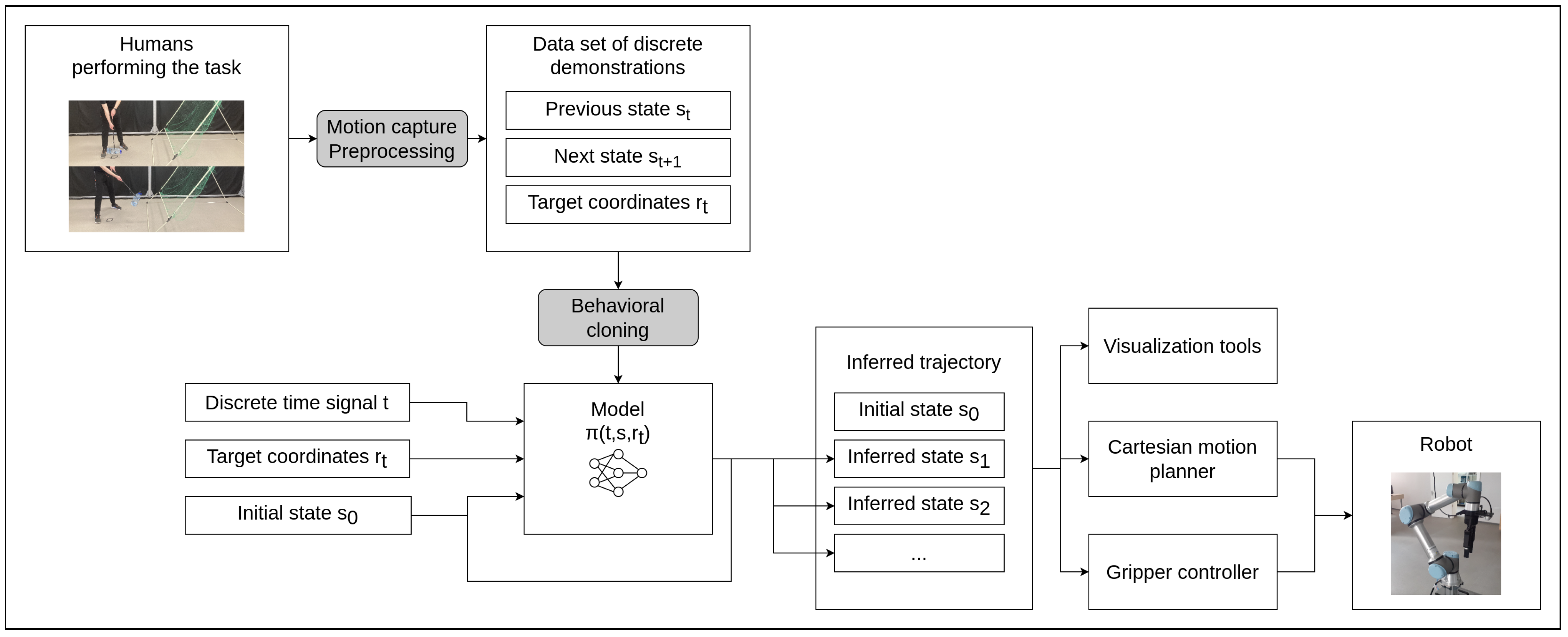
Ultimately, the approach selected (see
Figure 1) is to use pose–pose policies with footprints given in Equation (
16). These predict sequences of states containing position and orientation in Cartesian space. Such sequences can then be used as inputs to Cartesian motion planning algorithms, which produce joint trajectories to control the robot, as described in
Section 2.
5. Implementation
The system devised in this paper can be broken down into three main sections—the collection of observations in the physical environment (
Section 5.1), a pipeline for turning raw observation data into structured demonstrations with additional control signals (
Section 5.2), and neural network model implementations (
Section 5.3). System performance was evaluated, and design feedback was obtained in two main ways. First, qualitative observations of the generated trajectories were made using spatial visualization in a virtual environment, followed by execution on simulated and real robots (
Section 5.4). When satisfactory performance was attained, a series of quantitative metrics were computed for comparing system outputs with training and validation datasets on different model architectures and hyperparameter sets (
Section 5.5).
5.1. Data Collection
All demonstrations were recorded using
OptiTrack equipment that consists of a set of cameras, highly reflective markers to be attached to trackable objects, and the
Motive software package, which handles pose estimation and streaming. As shown in
Figure 2, a cage with eight cameras installed serves to hide external sources of specular reflections from the cameras and confine moving objects, such as drones, from leaving the scene. To simulate an industrial robot end effector, a gripping hand tool was equipped with markers. Since the motivating application calls for throwing plastic bottles, one such one was also marked for extrapolating target coordinates and identifying the release point in a demonstration. A start point was laid down on the floor to serve as a datum for automatically separating the recorded demonstrations during pre-processing. Holding the effector stand-in here for at least a second before each demonstration provided a consistent signal that can be identified programmatically.
Nets were used to catch the thrown bottle and prevent damaging the markers. These were also marked to aid in delimiting the ballistic segment of the thrown object’s flight. While in principle it is possible to detect an object in freefall by observing its acceleration, for trajectory extrapolation, this was deemed too prone to error—some impacts radically change the horizontal component of the object’s velocity without breaking its fall, and the acceleration of the empty bottles proved to be affected by air resistance to a significant degree, owing to their low terminal velocity.
In software, rigid body definitions were created for all objects to be tracked. These were then streamed on the local network, relayed over
robot operating system (ROS) topics corresponding to each rigid body using a pre-existing package ROS and recorded into a bag file to be converted into a .csv data set. Over the course of this project, two data sets with roughly 150 and 50 demonstrations each were collected. The first was used in the development process but proved to contain throws beyond the capabilities of the robot hardware used. Therefore, a second data set of throws with less pronounced swings was produced to fit within the working volume of the robot arm. A notable feature of the second data set is that initial orientations were randomized to a much lesser degree (
) than in the original corpus (
), and the range of estimated target coordinates for the throws was also more tightly constrained (
m along the
x-axis as opposed to
m), likely contributing to the better estimated throw accuracy metrics as illustrated in
Section 6.
5.2. Pre-Processing, Extraction of Implicit Control Signals
Figure 3 provides a schematic overview of the main steps involved in the data preparation process. For illustrative purposes, graphs of the effector
x-coordinate with respect to time are used, but the final picture also contains the estimated target coordinate of each throw.
After each recording session, an entirely unstructured corpus is available. It contains timestamped pose observations collected at whatever intervals they happened to have been generated by the tracking software. Each observation only contains information about a single tracked body. A peculiarity of this particular recording method is that observations about each body tend to arrive in bursts:
where
corresponds to the observed state of object
a at time
t. Thus, to obtain sequential data in discrete time, it is necessary to resample the positions and orientations of all relevant bodies at a constant time step:
A sampling frequency of 100 Hz was selected to obtain spatial precision on the order of centimeters given the velocities involved. Fortuitously, the intervals between observed bursts in the actual data are generally on this order as well. Resampling is accomplished using forward fill interpolation, which introduces a slight sawtooth oscillation, but this is removed in the subsequent smoothing step along with other discontinuities.
After resampling, individual demonstrations are separated using the aforementioned consistent starting position. This may vary from recording session to recording session, so it needs to be identified and configured manually. Specifically, the condition used to identify demonstration start points is as follows:
which is to say that every observation no more than
steps before
has to lie within
of the datum
. Each demonstration then consists of observations
The constants are determined experimentally to produce consistent observations for the particular task and may require tuning if the manner in which demonstrations are recorded changes. The newly split demonstrations are saved in separate files, thus allowing demonstrations generated in different sessions to be processed at once.
As further thresholding steps rely on estimates of pose derivatives, a smoothing step is first employed to remove noise and the slight sawtooth oscillation induced by the resampling step. This is accomplished by applying a rolling average kernel to the trajectory. Nevertheless, it was found that any estimate of derivatives would exacerbate what noise there was in the dataset, leading to inconsistent results. So a simplified estimator
, combining a correlate of the derivative
with a rolling average filter, was used with satisfactory results:
This was then used to compute threshold functions corresponding to the start of motion, actuator release and unfettered freefall of the bottle:
where
corresponds to the position component of the observation vector. Note that in the first case, the norm of a vector derivative is used, whereas in the subsequent two it is the scalar derivative of a vector norm. As discussed in
Section 5.1, the other terminating condition for the freefall segment of the bottle’s trajectory is determined using the position of the net:
The particular contents of the thresholding functions used are application-specific, but the method of detecting discrete events based on relative and absolute derivatives should prove to be broadly applicable. As with the split step, constants for thresholding were determined by way of inspection and would certainly be unique to each type of task. The output of
serves as the gripper actuator signal estimate.
is used in the final align, crop, and combine steps to determine the first observation to include in the dataset.
are used in estimating the desired target coordinates of each throw to give models the capability to be aimed. This is done by applying quadratic regression to the
z-coordinate of the object thrown, finding its intersection with the ground plane in corresponding
x and
y-coordinates—a geometric illustration of this process can be found in
Figure 4. The actuator signal and target coordinates are concatenated to each observation vector, with target coordinates being constant within each demonstration. A time signal is also added to each observation, as this was found to improve the performance of feedforward models. Finally, when combining the demonstrations into a training data set, all position vectors are shifted so that the start of motion corresponds to the origin of the coordinate system. This way, the models are trained to operate relative to the effector starting position.
5.3. Models
We studied two classes of parametric models as part of this project—simple feedforward neural networks and RNNs, operating autoregressively. The choice was motivated by two factors:
The dynamics of the problem were deemed to be simple enough that even small models would be able to model them adequately—making it possible to quickly train on development machines with low parameter counts, using pre-existing code libraries;
Given the recent advances in employing sequence-to-sequence models for imitation learning tasks, it was decided that models with broadly similar footprints and characteristics should be used to enable further research in this direction.
After an initial hyperparameter discovery process, the values in
Table 1 were arrived at for both model types, respectively. A range of model sizes and training epoch counts was compared for both models. In the case of the recurrent neural network, performance with different learning rates was also evaluated. As the feedforward models were developed first, performance with and without a time signal in the input data was also compared. For the RNN architecture, a
gated recurrent unit (GRU) was selected, as prior research suggests that it outperforms
long short-term memory (LSTM) when dealing with small data sets of long sequences [
28].
The basic model footprint is given as follows:
where
represent the end effector translation vector, orientation quaternion and gripper actuator signal, respectively, at time step
t in both the input and output. The input is augmented with a time/phase signal (discrete time step divided by the sampling frequency, in this case 100 Hz) relative to the start of the demonstration or generated trajectory, as well as the target coordinate vector
, which corresponds to the extrapolated target coordinates in the demonstration data set and commanded throw coordinates at inference. The time signal was added to the input, as it was found that trajectories generated by feedforward networks were liable to diverge without it, and the data sets thus modified were used for all training thereafter. The gripper control signal has values
in the training data set.
For training both types of networks, state transitions are constructed. In the case of the feedforward network, these state transitions are then shuffled and batched independently. For the RNN, pairs of feature-label sequences are formed corresponding to complete demonstrations, and the loss function is computed on the entire predicted output sequence. To hold these variable-length sequences, a ragged tensor is used, which is batched along its first axis and ragged along the second. With both types of networks, the Huber loss function is utilized.
5.4. Visualization and Execution
As discussed in the introduction, an important part of the reason for selecting throwing as our motivating application is the fact that it is easy for humans to judge the qualitative performance aspects of this task. To accomplish this, a means of visualizing the model outputs was required. When operating in open-loop mode (without interfacing with the physical or simulated environment—running the model on its previous outputs) it is possible to precompute trajectories and simply save them as sequences of robot states. To aid in estimating whether these trajectories were feasible, a tool for visualizing these sequences in the robot coordinate system was developed (
Figure 5a).
Given a policy that synchronously predicts the state of the system at the next time step, there are multiple possible ways to use it in robot control. The simplest approach is static trajectory planning—precompute a sequence of states and plan the motion between them. This is somewhat hindered by the lack of existing tools for precise time-parametrized Cartesian path planning in the ROS ecosystem. An alternative is a real-time pose following servo controller. The advantage of the latter approach is that closed-loop control is possible—with state observations taken from the environment, potentially allowing the model to compensate for offsets in real-time. However, this presents the challenge of tuning controller gains. The method that was ultimately employed was open-loop planning of Cartesian paths—with timing approximated through a combination of time-optimal trajectory generation [
11], followed by scaling the trajectory to the correct total duration. To control the gripper, a threshold value was set, the point in the trajectory at which this value was crossed was found, the corresponding joint state was computed, and a callback function was set up to trigger when this joint state was reached within an angular tolerance of 0.05 radians for each joint independently.
While this is adequate for evaluating the positioning of the generated trajectories and approximates the velocity profile closely enough for successful throws to be executed (
Figure 5b), a fully-featured time-parametrized Cartesian path planner or correctly tuned pose-following controller would be required to judge the throwing accuracy on real hardware and generalize our approach to other tasks. However, the development of such general-purpose tools was deemed to be outside the scope of this project, the focus of which is on the collection of demonstration data and imitation learning methods.
5.5. Evaluation Metrics
To draw comparisons between models of different architectures developed as part of our work, trained with differing hyperparameter sets, quantitative evaluations needed to be computed. As this is not a standard task with agreed-upon metrics and benchmarks, some exploratory work was required to arrive at quantifiers that agree with intuitively self-evident characteristics. While in principle it should be possible to judge models based on throw accuracy, this is not very helpful in the early stages of research when most models fall short of attaining the desired objective. Furthermore, limitations imposed by the aforementioned time parametrization issues with Cartesian motion planning in ROS make such a comparison as yet infeasible.
Hence, it was decided to compare model outputs with the demonstration data set. As judging against the training data set only informs us to the extent to which the model has been able to overfit, a smaller validation data set was set aside for out-of-distribution comparisons. The outputs to be compared were obtained by executing the models autoregressively on each demonstration’s initial state for as many steps as were present in the corresponding recorded demonstration. This can be formally stated as
where
refers to the evaluation data set of a single model with respect to either the validation or test demonstration set, but
are the demonstration and generated trajectories (sequences of state observations
) sharing the same initial state respectively.
Three broad classes of evaluation metrics were computed: data set-wise (global), step-wise and throw parameters. The first consists of vector similarity measures, such as Pearson’s correlation coefficient, cosine similarity and distance metrics applied to the entire data set and the trajectories generated against it as concatenated vectors:
The second class involves applying various measures to the observation/state variables at each time step:
where the inner function
g corresponds to metrics such as position error, rotation error (quaternion angular distance), or categorical cross-entropy in the release signal. Finally, a release error metric was computed trajectory-wise. To do this, the release point of each trajectory was found, the corresponding position found and the velocity vector estimated. When considering ways to combine these two terms into a single quantitative error estimator, it was decided that a simple ballistic extrapolation and resulting miss distance along the ground plane would serve as a decent first-order approximation of throw accuracy
vis-à-vis the training or validation data set.
Specifically, the release position
and estimated release velocity
were used as parameters in the equations:
The ground plane intersect time
was found by setting Equation (
21) equal to the ground plane coordinate
and finding the positive root. Then ground plane intersect points were found as
and the trajectory-wise throw error metric computed by
with
being the demonstration and generated throw intersect positions, respectively. Seeing as not every model would output a release signal that crosses the threshold (0.5) for every trajectory, this error term was set to be infinite in cases when no throw was defined.
6. Results
In our research, numerous models were trained on both of the data sets described in
Section 5.1, in both of the architectures discussed in
Section 5.3. After the initial trial and error process, a systematic training regimen produced the following:
Feedforward networks—a total of 48 models, varying the training data set, presence of a time signal in the features, perceptron counts per hidden layer, and training duration;
RNNs—36 models with data set, learning rate, model size, and training length being the variable parameters.
Figure 5 illustrates how model outputs were visualized to use their qualitative aspects in guiding hyperparameter choice, and a preliminary implementation on a real robot was achieved—executing trajectories generated by the simpler feedforward network, with target coordinates sampled from normal distributions corresponding to their values in the training data set. As can be seen, when these outputs were used to generate motion plans for a
Universal Robots UR5e robot equipped with a pneumatic gripper, a plastic bottle was successfully thrown into a target container located outside the robot’s reachable volume. Adequate output sequences were attained with both model architectures at multiple hyperparameter combinations, so to draw specific conclusions, the quantitative evaluation metrics discussed in
Section 5.5 were produced for the 84 systematically trained models described above. Of the feedforward models, 18 out of 48 (37.5%) successfully triggered a gripper release on every evaluation trajectory, enabling mean throw error estimates to be computed. Among the RNNs, this was true for 24 out of 36 (66.7%).
Figure 6 shows a broad comparison between the RNN and feedforward model architectures, with each of the evaluation metric classes being present, though not all the specific metrics discussed—as there was found to be a considerable amount of duplication in their findings. All figures shown correspond to the best result attained by either type in each of the performance indicators, irrespective of other variables.
Figure 7 elaborates upon each model class, showing the best attained results at various hyperparameter values. In the case of the feedforward model, the input observations did not initially contain a time signal, which was rectified early on. In the case of the RNN, deviating from the default learning rate was found to be beneficial. For both architectures, the best performance at each epoch count and parameter count is also plotted.
Figure 8 shows the impact of only varying the crucial size (perceptron count)—in each case, the two best performing models at each fixed parameter combination are selected and their performance at different values of the independent variable is graphed.
7. Discussion
The qualitative aspects of our results—the visual representations of trajectories and their characteristics when executed on a real robot—closely resemble throwing motions as executed by the human experts, suggesting that the selected approach to data collection is adequate for encoding the key features of this task. The same can be said for the fact that a large minority of the feedforward models and a majority of the recurrent ones were able to reproduce a complete throw trajectory for every set of initial conditions in the training and validation data sets. The most important takeaway regarding this aspect of our approach is that augmenting the data with time step information is important to achieve good performance.
Comparing the two proposed model architectures by their best attained values, in terms of distribution similarity measures such as cosine similarity and Euclidean distance, the results are generally quite good for both, with the RNN having the edge in most distance measures but notably one of the feedforward models demonstrating the highest cosine similarity. In terms of step-wise metrics, RNN models typically show better results—which is perhaps to be expected, given that their inputs contain all previous states in the trajectory rather than a single observation.
The same is true for the throw error metric in general, and it is quite apparent when comparing the percentage of valid throw trajectories (ones where actuator release has been commanded) that RNNs have an overall easier time learning the release timing aspect of the task. However, the best single result was attained by an outlier feedforward model—an average error of around 0.09 m, as opposed to around 0.11 m for the best recurrent model—both on the validation data taken from the corrected, smaller demonstration collection (see
Section 5.1). This result should be taken with a grain of salt, though, considering the small size of the validation data set (5 demonstrations, set aside from a collection of 45). The performance of the same feedforward model compared against the remaining training data set is much worse—an error of 0.57 m—compared to the best RNN model, which retains an error of 0.26 m. Moreover, at other hyperparameter combinations, RNN models can be seen to retain a sub-0.2 m error on both data sets (such as a 256-perceptron model trained for 300 epochs at a learning rate of
, which attains 0.16 m and 0.18 m error on the training and validation data sets, respectively).
An important thing to note is that this throw error estimate should not be taken as equivalent to a simulation or an actual throw—as was already discussed in
Section 5.1, the terminal velocities of the bottles thrown are low enough to affect the observed trajectories, and in any case, instantaneous velocity vector estimates derived from sequences of discrete position measurements are bound to have a degree of error. This is further exacerbated by the fact that the interactions between the gripper and the work object would impart some delay between the release command and full separation. Nevertheless, this estimator does model a large part of the non-linear relationship between the parameters that define a throw—release position and velocity vectors—in a way that is likely to explain a large degree of destination variance among throws performed in the physical world. It is reasonable to assume that lower values of this error term would be strongly correlated with higher accuracy when deployed and tested on physical hardware.
Regardless of model type and parameters, the observed performance on the older data set, uncorrected for robot working volume—with a much greater variance in throw shape, timing, starting orientation, and target coordinates, but only marginally greater size—is significantly worse. None of the feedforward networks attain a throw error estimate under 0.6 m, while RNNs bottom out at around 0.4 m. In the case of feedforward networks, augmenting the input vector with a time signal showed qualitatively observable advantages, and these are also present in the numeric evaluations. An apparent trend of better results being obtainable with smaller models that are not trained for too long also exists; however, for the reasons discussed above, this may well be spurious. Certainly, no such conclusion can be confidently drawn with respect to the RNNs’ performance, as comparatively high performance is achieved by some hyperparameter combinations at every scale explored. A slight, but consistent edge in estimated throw error performance was attained by increasing the learning rate of the Adam optimizer from the default value of to . It is notable, however, that lower learning rates appear to produce higher similarity metrics.
Observing the impact of hyperparameters in isolation yields the clearest insights in the cases of global distribution similarity measures (in the graphs shown, cosine similarity). In feedforward models, a high similarity is attained, even at the lowest parameter counts, and making the models larger does not yield unambiguous improvements. Notably, at some settings, there is a considerable degree of variance in this metric—at 1024 perceptrons per layer, the highest cosine similarity is attained by a model trained without the time signal, which performs notably worse at other sizes. Among RNNs, the perceptron counts examined show a slightly yet still monotonically increasing trend, suggesting that performance gains at larger model sizes may still be made. When it comes to throw accuracy estimates, neither model architecture shows a clear response to perceptron count, and the feedforward architecture again exhibits outlier results. Interestingly, multiple RNN configurations show initially declining performance on validation data with increased model size, followed by an improvement—potentially evoking the double descent phenomenon [
29]. However, there is still a comparable degree of unexplained variance in the results, which forces us to be cautious in proposing any concrete explanations.
8. Conclusions
The original goal we set out to accomplish was to devise a framework for recording demonstrations by human actors and using these to execute an object-throwing task as a stand-in for a variety of similar future applications. In this, we were mostly successful—using motion capture as the data collection mechanism, it proved possible to employ a series of analytic pre-processing steps to turn raw recording data into demonstration data sets suitable for training two varieties of artificial neural networks—feedforward and recurrent. The models were structured to be able to operate either in-the-loop or autoregressively as forward planners, and it was this latter approach that was further explored—we developed tools for their visualization (useful in hyperparameter discovery) and prototype motion planning software that enable execution on real robots. Model outputs were used to successfully perform throws in the physical world.
The data collection step with motion capture equipment proved to be straightforward to customize for our motivating application. However, it did require some attention to how the physical demonstrations were performed—with allowances for automatic demarcation of distinct demonstrations. A pre-processing pipeline had to be developed to extract these separate trajectories and only their relevant segments, as well as inferring hidden state variables through indirect observation. While the latter are likely going to be specific to each application, the methods herein can be trivially adapted so long as these can be expressed as n-th order derivatives of absolute or relative pose variables of tracked objects in the scene. Admittedly, some work, such as target coordinate extrapolation, was entirely specific to this task.
In contrast to some previous work that has explored motion capture in imitation learning, we place a greater emphasis on using general-purpose machine learning methods—artificial neural networks—to generate the trajectories at inference, as opposed to simple neighbor methods [
20] or highly domain-specific approaches grounded in the use of dynamic motion primitives [
21]. To more objectively evaluate the performance of the policies obtained with various hyperparameters and on different data sets, a series of quantitative metrics are proposed in this paper. In general, it can be said that, according to these, recurrent networks operating on complete state histories outperform simple deep neural networks operating in a Markovian regime—which is perhaps unsurprising, given the recent successes achieved in applying general-purpose sequence-to-sequence learning methods to the imitation learning domain [
19]. As our model precision comparisons rely on indirect estimates rather than empirical data, it is hard to make a direct comparison with state-of-the-art performers in throwing tasks, such as [
26], but it should be noted that they use learning at a higher level—outputting parameters that describe each throw—and do not use model outputs to generate Cartesian motion plans directly as proposed here. This makes their entire approach inherently more coupled to a single type of task than ours.
Potential directions for further research and engineering work based on what we have achieved thus far would be the following:
Replacement of simple feedforward neural networks with generative adversarial models, which demonstrate some of the best performance for pure Markovian policies [
15]. This way, the need for more compute-intensive sequence-to-sequence models that necessitate keeping track of state histories may be obviated;
Adapting the pipeline for other tasks of interest, mainly to explore how easily the data pre-processing pipeline generalizes in practice;
Train models to predict velocities as the actions, rather than subsequent states, for integration with servo controllers;
Development of a Cartesian arrival-time parametrization tool in ROS, something which is currently lacking in the ecosystem.
Author Contributions
Conceptualization, P.R., J.A. and M.G.; methodology, P.R.; software, P.R.; validation, P.R.; formal analysis, P.R.; investigation, P.R.; resources, J.A. and P.R.; data curation, P.R.; writing—original draft preparation, P.R.; writing—review and editing, J.A. and M.G.; visualization, P.R.; supervision, M.G.; project administration, J.A.; funding acquisition, M.G. All authors have read and agreed to the published version of the manuscript.
Funding
This work is conducted under the framework of the ECSEL AI4DI and VIZTA projects, funded from the ECSEL Joint Undertaking (JU) under grant agreements No 826060, No 826600.
Institutional Review Board Statement
Not applicable.
Informed Consent Statement
Informed consent was obtained from all subjects involved in the study.
Data Availability Statement
Conflicts of Interest
The authors declare no conflict of interest. The funders had no role in the design of the study; in the collection, analyses, or interpretation of data; in the writing of the manuscript, or in the decision to publish the results.
References
- Arents, J.; Greitans, M. Smart industrial robot control trends, challenges and opportunities within manufacturing. Appl. Sci. 2022, 12, 937. [Google Scholar] [CrossRef]
- Sutton, R.S.; Barto, A.G. Reinforcement Learning: An Introduction; MIT Press: Cambridge, MA, USA, 2018; pp. 60–77. [Google Scholar]
- Hester, T.; Vecerik, M.; Pietquin, O.; Lanctot, M.; Schaul, T.; Piot, B.; Horgan, D.; Quan, J.; Sendonaris, A.; Osband, I.; et al. Deep q-learning from demonstrations. In Proceedings of the Thirty-Second AAAI Conference on Artificial Intelligence, New Orleans, LA, USA, 2–7 February 2018. [Google Scholar]
- Abbeel, P.; Ng, A.Y. Apprenticeship learning via inverse reinforcement learning. In Proceedings of the Twenty-First International Conference on Machine Learning, Banff, AB, Canada, 4–8 July 2004; p. 1. [Google Scholar]
- Attia, A.; Dayan, S. Global overview of imitation learning. arXiv 2018, arXiv:1801.06503. [Google Scholar]
- Zhang, T.; McCarthy, Z.; Jow, O.; Lee, D.; Chen, X.; Goldberg, K.; Abbeel, P. Deep imitation learning for complex manipulation tasks from virtual reality teleoperation. In Proceedings of the 2018 IEEE International Conference on Robotics and Automation (ICRA), Brisbane, Australia, 21–25 May 2018; pp. 5628–5635. [Google Scholar]
- Dyrstad, J.S.; Øye, E.R.; Stahl, A.; Mathiassen, J.R. Teaching a robot to grasp real fish by imitation learning from a human supervisor in virtual reality. In Proceedings of the 2018 IEEE/RSJ International Conference on Intelligent Robots and Systems (IROS), Madrid, Spain, 1–5 October 2018; pp. 7185–7192. [Google Scholar]
- Liu, Y.; Gupta, A.; Abbeel, P.; Levine, S. Imitation from observation: Learning to imitate behaviors from raw video via context translation. In Proceedings of the 2018 IEEE International Conference on Robotics and Automation (ICRA), Brisbane, Australia, 21–25 May 2018; pp. 1118–1125. [Google Scholar]
- Rumelhart, D.E.; Hinton, G.E.; Williams, R.J. Learning Internal Representations by Error Propagation; Technical Report; California University of San Diego La Jolla Institute for Cognitive Science: La Jolla, LA, USA, 1985. [Google Scholar]
- Vaswani, A.; Shazeer, N.; Parmar, N.; Uszkoreit, J.; Jones, L.; Gomez, A.N.; Kaiser, Ł.; Polosukhin, I. Attention is all you need. In Proceedings of the Advances in Neural Information Processing Systems, Long Beach, CA, USA, 4–9 December 2017; pp. 5998–6008.
- Kunz, T.; Stilman, M. Time-optimal trajectory generation for path following with bounded acceleration and velocity. Robotics: Science and Systems VIII; MIT Press: Cambridge, MA, USA, 2012; pp. 209–216. [Google Scholar]
- Pomerleau, D.A. Alvinn: An Autonomous Land Vehicle in a Neural Network; Technical Report; Carnegie-Mellon University of Pittsburgh Pa Artificial Intelligence and Psychology: Pittsburgh, PA, USA, 1989. [Google Scholar]
- Pastor, P.; Hoffmann, H.; Asfour, T.; Schaal, S. Learning and generalization of motor skills by learning from demonstration. In Proceedings of the 2009 IEEE International Conference on Robotics and Automation, Kobe, Japan, 12–17 May 2009; pp. 763–768. [Google Scholar]
- Ross, S.; Gordon, G.J.; Bagnell, J.A. No-regret reductions for imitation learning and structured prediction. In Proceedings of the AISTATS, Citeseer, Fort Lauderdale, FL, USA, 11–13 April 2011. [Google Scholar]
- Ho, J.; Ermon, S. Generative adversarial imitation learning. Adv. Neural Inf. Process. Syst. 2016, 29, 4565–4573. [Google Scholar]
- Torabi, F.; Warnell, G.; Stone, P. Generative adversarial imitation from observation. arXiv 2018, arXiv:1807.06158. [Google Scholar]
- Scherzinger, S.; Roennau, A.; Dillmann, R. Contact skill imitation learning for robot-independent assembly programming. In Proceedings of the 2019 IEEE/RSJ International Conference on Intelligent Robots and Systems (IROS), Macao, China, 3–8 November 2019; pp. 4309–4316. [Google Scholar]
- Lynch, C.; Khansari, M.; Xiao, T.; Kumar, V.; Tompson, J.; Levine, S.; Sermanet, P. Learning latent plans from play. In Proceedings of the Conference on Robot Learning, Cambridge, MA, USA, 16–18 November 2020; pp. 1113–1132. [Google Scholar]
- Reed, S.; Zolna, K.; Parisotto, E.; Colmenarejo, S.G.; Novikov, A.; Barth-Maron, G.; Gimenez, M.; Sulsky, Y.; Kay, J.; Springenberg, J.T.; et al. A Generalist Agent. arXiv 2022, arXiv:2205.06175. [Google Scholar]
- Jha, A.; Chiddarwar, S.S.; Bhute, R.Y.; Alakshendra, V.; Nikhade, G.; Khandekar, P.M. Imitation learning in industrial robots: A kinematics based trajectory generation framework. In Proceedings of the Advances in Robotics, New Delhi, India, 28 June–2 July 2017; pp. 1–6. [Google Scholar]
- Vuga, R.; Ogrinc, M.; Gams, A.; Petrič, T.; Sugimoto, N.; Ude, A.; Morimoto, J. Motion capture and reinforcement learning of dynamically stable humanoid movement primitives. In Proceedings of the 2013 IEEE International Conference on Robotics and Automation, Karlsruhe, Germany, 6–10 May 2013; pp. 5284–5290. [Google Scholar]
- Fragkiadaki, K.; Levine, S.; Felsen, P.; Malik, J. Recurrent Network Models for Human Dynamics. In Proceedings of the IEEE International Conference on Computer Vision (ICCV), Santiago, Chile, 7–13 December 2015. [Google Scholar]
- Pavllo, D.; Grangier, D.; Auli, M. Quaternet: A quaternion-based recurrent model for human motion. arXiv 2018, arXiv:1805.06485. [Google Scholar]
- Ude, A.; Gams, A.; Asfour, T.; Morimoto, J. Task-specific generalization of discrete and periodic dynamic movement primitives. IEEE Trans. Robot. 2010, 26, 800–815. [Google Scholar] [CrossRef] [Green Version]
- Park, S.; Kim, J.; Kim, H.J. Zero-Shot Transfer Learning of a Throwing Task via Domain Randomization. In Proceedings of the 2020 20th International Conference on Control, Automation and Systems (ICCAS), Busan, Korea, 13–16 October 2020; pp. 1026–1030. [Google Scholar]
- Zeng, A.; Song, S.; Lee, J.; Rodriguez, A.; Funkhouser, T. Tossingbot: Learning to throw arbitrary objects with residual physics. IEEE Trans. Robot. 2020, 36, 1307–1319. [Google Scholar] [CrossRef]
- Höfer, S.; Bekris, K.; Handa, A.; Gamboa, J.C.; Mozifian, M.; Golemo, F.; Atkeson, C.; Fox, D.; Goldberg, K.; Leonard, J.; et al. Sim2Real in robotics and automation: Applications and challenges. IEEE Trans. Autom. Sci. Eng. 2021, 18, 398–400. [Google Scholar] [CrossRef]
- Yang, S.; Yu, X.; Zhou, Y. Lstm and gru neural network performance comparison study: Taking yelp review dataset as an example. In Proceedings of the 2020 International Workshop on Electronic Communication and Artificial Intelligence (IWECAI), Qingdao, China, 1–3 June 2020; pp. 98–101. [Google Scholar]
- Nakkiran, P.; Kaplun, G.; Bansal, Y.; Yang, T.; Barak, B.; Sutskever, I. Deep double descent: Where bigger models and more data hurt. J. Stat. Mech. Theory Exp. 2021, 2021, 124003. [Google Scholar] [CrossRef]
Figure 1.
A high-level overview of the proposed approach. Demonstrations are recorded with motion capture equipment, a split and cropped data set augmented with target coordinates, and a gripper actuation signal is created. This is used to train neural network models in behavioral cloning. When operating in the open-loop regime, prior model outputs are used to autoregressively predict subsequent states. The resulting sequence can then be fed into a Cartesian motion planner to control a robot.
Figure 2.
Motion capture equipment and demonstration acquisition process.
Figure 2.
Motion capture equipment and demonstration acquisition process.
Figure 3.
Pre-processing pipeline overview. All charts are purely illustrative and show effector x-axis position with respect to time (in blue). The final diagram also shows the target x-coordinate of each discrete demonstration (in red). The thresholds are, from left to right: movement, release, freefall start and freefall end.
Figure 4.
Estimation of the throw target coordinates. Bottle position data are used to annotate each demonstration—consisting of effector pose observations—with throw target coordinates. Regression on the z-axis is used to find the ground plane intersection time, at which extrapolated x- and y-coordinate values are found.
Figure 5.
Qualitative performance evaluation—visualization and execution. In both cases, the trajectories were sequences of pose (position, orientation) goals obtained by running the models autoregressively on their outputs at prior time steps. Release timing is represented in (a) by the change in marker size.
Figure 6.
Results—comparison between model architectures (Naive—refers to the feedforward architecture, also “naive behavioral cloning”), the best performance attained in each class. Top row metrics—cosine similarity (dimensionless), Euclidean distance (all features, no specific unit); mean position error (stepwise, meters). Bottom row—mean rotation error (stepwise, radians), mean throw error (meters).
Figure 7.
Results—best mean throw error performance for each hyperparameter value, in units of meters. The top row shows feedforward model results, the bottom—RNN. In both cases, the smaller, newer dataset with less variance in orientation and target coordinates results in better throw evaluations. Introducing the time signal significantly improves feedforward model performance, whereas for the RNN, improved results could be attained at higher learning rates. In the case of the feedforward model, training for too long and making the model too large initially appears to be detrimental, while for the RNN, no clear trend was observed in this respect.
Figure 8.
Results—cosine similarity (dimensionless) and mean throw error (meters) metrics for feedforward and recurrent models, only varying in the perceptron count parameter (others held constant)—best 2 on train and validation sets each.
Figure 8.
Results—cosine similarity (dimensionless) and mean throw error (meters) metrics for feedforward and recurrent models, only varying in the perceptron count parameter (others held constant)—best 2 on train and validation sets each.
Table 1.
Model hyperparameters.
Table 1.
Model hyperparameters.
| Parameter | Feedforward | RNN |
|---|
| Architecture | 2 dense hidden layers, ReLU | GRU, dense linear output |
| Parameter counts | 128–1024 perceptrons per layer | 128–512 perceptrons in the unit |
| Training epochs | 20–100 | 300–1200 |
| Batch size | 64 | 32 |
| Optimizer | Adam | Adam |
| Learning rate | | |
| Publisher’s Note: MDPI stays neutral with regard to jurisdictional claims in published maps and institutional affiliations. |
© 2022 by the authors. Licensee MDPI, Basel, Switzerland. This article is an open access article distributed under the terms and conditions of the Creative Commons Attribution (CC BY) license (https://creativecommons.org/licenses/by/4.0/).


