Article

Groundwater Contaminant Transport Solved by Monte Carlo Methods Accelerated by Deep Learning Meta-Model

Institute of New Technologies and Applied Informatics, Faculty of Mechatronics, Informatics and Interdisciplinary Studies, Technical University of Liberec, Studentská 1402/2, 461 17 Liberec, Czech Republic
*
Author to whom correspondence should be addressed.
Appl. Sci. 2022, 12(15), 7382; https://doi.org/10.3390/app12157382
Submission received: 19 June 2022 / Revised: 12 July 2022 / Accepted: 15 July 2022 / Published: 22 July 2022
(This article belongs to the Special Issue Monte Carlo Simulation in Quantum Science and Applied Physics)

Abstract

:
Groundwater contaminant transport modeling is a vitally important topic. Since modeled processes include uncertainties, Monte Carlo methods are adopted to obtain some statistics. However, accurate models have a substantial computational cost. This drawback can be overcome by employing the multilevel Monte Carlo method (MLMC) or approximating the original model using a meta-model. We combined both of these approaches. A stochastic model is substituted with a deep learning meta-model that consists of a graph convolutional neural network and a feed-forward neural network. This meta-model can approximate models solved on unstructured meshes. The meta-model within the standard Monte Carlo method can bring significant computational cost savings. Nevertheless, the meta-model must be highly accurate to obtain similar errors as when using the original model. Proposed MLMC with the new lowest-accurate level of meta-models can reduce total computational costs, and the accuracy of the meta-model does not have to be so high. The size of the computational cost savings depends on the cost distribution across MLMC levels. Our approach is especially efficacious when the dominant computational cost is on the lowest-accuracy MLMC level. Depending on the number of estimated moments, we can reduce computational costs by up to ca. 25 % while maintaining the accuracy of estimates.

1. Introduction

Groundwater quality might be affected by many natural and industrial processes. There are many sources of groundwater contamination, for instance, polluted precipitation, runoff from roadways, leaking barrels of waste chemicals, etc. [1] (p. 500). High concentrations of dissolved substances can result in water being unfit for drinking or irrigation. Our research focuses on observing groundwater processes in the vicinity of a deep geological repository (DGR) of radioactive waste. Despite all the protective layers, radioactive material will be exposed to the geosphere in the distant future. As a result, groundwater may become contaminated. Since it is not feasible to measure these processes directly, we model and simulate them numerically. Taking the uncertainties into account, we consider bedrock properties as random variables, specifically, spatially correlated random fields (SRF). Consequently, a quantity of interest (QoI) is also a random variable. We investigate statistical moments of a QoI in the first place and a probability density function (PDF) afterward.
Models can be process-based or data-driven [2] (p. 4). Our research takes advantage of both approaches. First, we run a stochastic process-based contaminant transport model. A physical process is numerically solved by the finite element method on an unstructured mesh with prescribed SRF. To estimate the expectation of QoI, the model run (=simulation) is performed multiple times in accordance with the Monte Carlo method (MC); for some applications, see [3,4,5]. However, MC suffers from high computational costs. Many highly accurate simulations must be performed to obtain statistical estimates with reasonably low variance, see [6] (p. 2). To save the cost, it is beneficial to construct a hierarchical system of less accurate but cheaper models that approximate the same QoI; for details, see [7] (p. 552). In the field of numerical modeling, the accuracy of a model is given by the number of mesh elements. Thus, we consider the hierarchy of models with gradually coarsened computational meshes, see [7] (p. 555). For this purpose, we adopt the multilevel Monte Carlo method (MLMC) [6] described in more detail in Section 4. For some MLMC applications, see [8,9,10,11].
A meta-modeling approach is another option for decreasing the total computational cost of MC. A function of inputs and parameters of a complex and expensive model is approximated by a simpler and faster meta-model, also called a surrogate model. Meta-modeling techniques are widely used across scientific fields (see [12]), and groundwater modeling is no exception [13,14,15,16]. In terms of the classification of meta-models by Robinson [17] and Asher et al. [13], we concentrate our effort on data-driven meta-models. In our case, the input of the model is a 2D SRF, and the output is some scalar QoI. Asher et al. [13] (p. 5958) also provides a list of popular data-driven meta-modeling techniques, such as radial basis functions, Gaussian processes, support vector regression (SVR), and neural networks (NN). For their brief description, see [18,19]. We have focused on meta-models based on neural networks, the applicability of which to hydrological processes was discussed in [20,21]. The latter article also provides the basics of deep learning and briefly introduces some popular DNN architectures. Neural networks and deep learning have already been utilized in groundwater modeling to predict its: level [22], quality [23,24], flow [25,26], or contaminant transport [27]. With regard to the nature of input data of our model, it would be felicitous to use a convolutional neural network (CNN) as a meta-model. CNNs excel in learning spatial relationships within data on a regular grid such as an image. Since we use unstructured meshes, we cannot adopt a CNN directly (see [28]). We briefly discussed some ways to overcome this difficulty in [29]. Representing the structure of SRF as a graph (for graph theory, see [30]) and then using a graph convolutional neural network (GCNN) [31] is the option we selected.
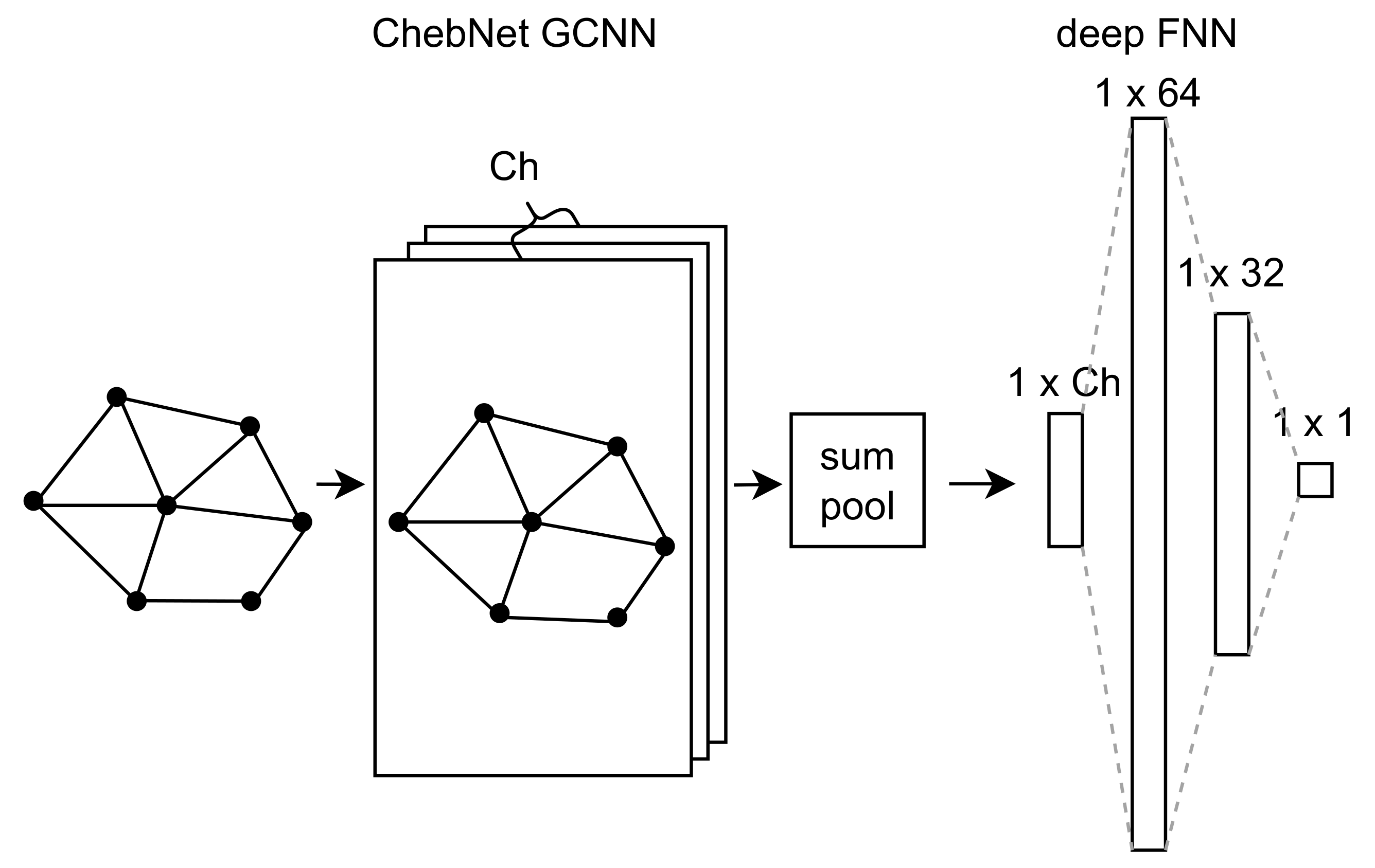
The general objective of the presented article is to reduce the computational cost of Monte Carlo methods by incorporating a meta-model. In this regard, we build on the findings of our initial article [29], which addressed the same objective with a GCNN meta-model of a groundwater flow problem. In this article, we specifically focus on improving the accuracy of the meta-model and its applicability for groundwater contaminant transport problems. To the best of our knowledge, no previous research in groundwater modeling has investigated the computational cost reduction in Monte Carlo methods using a meta-model.
The article is organized as follows. First, the contaminant transport model is described. Next, its deep learning meta-model is presented in Section 3. The multilevel Monte Carlo method is briefly introduced, and the proposed incorporation of the meta-model is delineated in Section 4 and Section 5. Section 6 is devoted to numerical experiments, meta-models are assessed, and their usage is put into the context of MC and MLMC. The article is concluded with a summary and discussion of the important findings.

2. Groundwater Contaminant Transport Model

We consider a conceptual 2D model of the transport of contaminants from DGR, see Figure 1. The Darcy flux of groundwater q [ms 1 ] is described by the equations:
div ( q ) = 0 , q = κ ( x ) p ,
where p is the pressure head [m], and κ is the hydraulic conductivity considered to be smaller at a stripe near the surface. The Darcy flow is driven by the seepage face condition:
( q · n ) p = 0 , q · n q 0 , p 0
on the top boundary, with q 0 denoting a precipitation flux. No flow is prescribed on the remaining boundaries. The surface geometry is intentionally overscaled to pronounce its impact on the groundwater flow.
The advection equation is used as the contaminant transport model:
t ( ϑ c ) + div ( q c ) = 0 ,
where ϑ is the porosity and c is the concentration [kg m 3 ] of a contaminant in terms of mass in the unit volume of water. The equation is solved for the unknown concentration with the initial condition c 0 = 1 in the repository and 0 elsewhere. Zero concentration is prescribed at the inflow part of the boundary.
The ϑ is given as a correlated random field. Then, the random field of hydraulic conductivity κ is determined from ϑ using the Kozeny–Carman equation and slight random scaling given by an independent random field. Figure 1 displays the geometry of the model, the random conductivity field (conductivity in the figure), and the concentration field (X_conc in the figure) at the time t = 3 of the total simulation time T = 20 . The simulation is performed using the Flow123d software [32].

3. Deep Learning Meta-Model

3.1. Graph Convolutional Neural Network Meta-Model

Graph neural networks (GNNs) are deep-learning-based models that operate on graph data [31]. They are adopted in many areas, including natural language processing, computer vision, bioinformatics, and physics. Similar to standard neural networks [33], they are categorized into several groups, such as graph convolutional neural networks (GCNN), graph attention networks, graph recurrent networks, etc. We employ GCNNs, which have a variety of different architectures. They can differ in many ways, such as the representation of a convolution operation, the size of a convolutional filter, the number of graph vertices taken into account, and many others. For a comprehensive survey on GCNNs, see [31,34].
In order to use GCNNs, the dual graph G = ( V , E ) of the computational mesh is considered with the vertices V corresponding to mesh elements and associated with the values of the input random fields. The edges correspond to the adjacent mesh elements. Figure 2 illustrates the graph representation of the SRF prescribed on an unstructured mesh.

3.2. ChebNet GCNN

After testing several architectures of GCNN, we ascertain that GCNN with the Chebyshev convolutional layer (ChebNet GCNN) [35] provides the best results in our case. It pertains to spectral GCNNs, which represent the graph convolution in terms of polynomials of a graph Laplacian matrix L.
For a brief general description, let G be the graph convolutional operator, x R | V | be a vector of input values associated with graph vertices, and g θ R K × C h be the convolutional kernel. The variable K stands for the maximal polynomial degree, and C h represents the number of channels of the kernel [33] (ch. 9). Then, the graph convolution of x and g θ is:
x G g θ = p θ K ( L ) x ,
where p is a polynomial of eigenvalues of L and has maximum degree K. When using ChebNet GCNN, p K ( L ) is defined via Chebyshev polynomials T k :
x G g θ = ( k = 0 K 1 θ k T k ( L ) ) x ,
where θ k R C h represents the learnable parameters of the kernel that are adjusted during the neural network learning procedure. The kernel is K-localized, i.e., the filtered signal at a particular vertex depends on information from vertices in its K-hop neighborhood. For a comprehensive explanation of GCNN, see [31] (p. 81).

3.3. Architecture of Meta-Model

Our deep learning meta-model consists of ChebNet GCNN followed by a deep feed-forward neural network (FNN) [33] (ch. 6). As depicted in Figure 3, the input graph enters the ChebNet GCNN with K = 4 and C h = 8 . The following global summation pool sums up information of all vertices for each channel. This flattened output of ChebNet GCNN forms the input to the deep FNN with two hidden layers of 64 and 32 neurons. To provide complete information about the neural networks employed, it is necessary to specify hyperparameters (generally about hyperparameters, see [33] (p. 120)). Our settings: Adam optimizer with learning rate 0.001 ; hidden layer activation function: ReLU; output activation function: identity; loss function: MSE; maximum number of epochs: 2000; and patience: 1000.

3.4. Assessment of Meta-Model

The following procedure was employed to assess different meta-models. Let D = { ( x i , c i ) } i = 1 D denote all available i.i.d. samples, x i R | V | be an input vector of the hydraulic conductivity values of an SRF, and c i R be the corresponding simulated concentration on the surface (see Section 2). Since we conduct supervised learning [33], D is divided into learning (=training) samples L and test samples T . Then, L is evenly divided into L s , s = 1 , , S to repeat the whole meta-model learning procedure S times. For each repetition, data are pre-processed to facilitate learning: c L s = ( c L s c L s ) / std 2 ( c L s ) , where std denotes the sample standard deviation.
Given L s , a meta-model learns a function f s ( x ) : R | x | R . The quality of the approximation is generally evaluated by a loss function, in our case, the mean squared error (MSE): λ ( M , f s ) = 1 | M | c M f s ( x M ) 2 2 , where M D . Namely, the training loss λ ( L s , f s ) and test loss λ ( T , f s ) are observed. For the sake of comparing the accuracy of different meta-models, we use the normalized root mean squared error ( N R M S E = M S E / std ). The training NRMSE J L = 1 S s = 1 S λ ( L s , f s ) std ( c L s ) and test NRMSE J T = 1 S s = 1 S λ ( T , f s ) std ( c T ) are calculated. This metric allows us to draw a comparison among models on different mesh sizes. The lower the NRMSE, the better. Moreover, if the NRMSE is above 1, we can use a simple random generator instead of a complex meta-model.

4. Multilevel Monte Carlo Method

The multilevel Monte Carlo method [6] (MLMC) is based on the variance reduction principle [6] (p. 3). Many simulation samples are collected at low levels, with less accurate but inexpensive approximations of the model available. While much fewer samples are collected at high levels, there are differences between approximations of the model that are more accurate but computationally expensive. If these differences have a significantly smaller variance, we obtain estimates with the same accuracy but at a fraction of the cost compared to the standard Monte Carlo method.
Let P be a random variable and P 1 , …, P L be a sequence of its approximations, where P l 1 P l . The approximations are becoming more accurate from P 1 to P L . Then, the expected value of P L satisfies the identity:
E [ P L ] = E [ P 1 ] + l = 2 L E [ P l P l 1 ] .
The MLMC estimates an individual expectation as follows:
P ^ = P 1 ( x n 1 ) N 1 + l = 2 L P l ( x n l ) P l 1 ( x n l ) N l ,
where L is the total number of levels, N l stands for the number of simulation samples on level l, N l denotes the average over N l samples. Pairs of random inputs ( x i l , x i l 1 ) are both discrete evaluations of a single realization of a random field x ( ω l , i ) , while the random states ω l , i are independent and come from a given probability space ( Ω , Σ , P ) .
When using estimator (7), we are particularly interested in its total computational cost C and estimated variance V ^ :
C = l = 1 L N l C l ,
V ^ = l = 1 L V ^ l N l ,
where C 1 , V ^ 1 denote the cost and the estimated variance of P 1 . Meanwhile, for l > 1 , C l , V l ^ represent the cost and the estimated variance of differences P l P l 1 . For a comprehensive MLMC theory, see [6].
In the presented way, it is feasible to estimate the expectations of quantities derived from the original QoI. In particular, we utilize the so-called generalized statistical moments of QoI. In our study, the moments’ functions ϕ ( x ) are Legendre polynomials, as they are suitable for the PDF approximation (see [36]).

4.1. Optimal Number of Samples

As previously mentioned, the principal motivation of our research is to reduce C. However, it is also essential to keep the variance of the estimator sufficiently low. To achieve this, we prescribe the target variance V t of the estimator. Then, the optimal N l is found by minimizing function (8) under the constraint
V t = l = 1 L V ^ l N l .
After some calculus:
N l r = V ^ l r C l i = 1 L V ^ i r C i V t , r = 1 , , R ,
where V ^ l r is an estimated variance of ϕ l r ( x ) ϕ l 1 r ( x ) for r th moment function on level l, ϕ 0 r = 0 . Finally, N l = max r = 1 , , R N l r . This procedure is crucial in our study and determines the results presented.
The Python library MLMC [37], developed by the authors of this article, is used to schedule simulation samples and post-process the results. The software also implements the maximal entropy method (MEM) to determine the PDF from moments estimated by MLMC. The description of MEM is beyond the scope of this article. The interested reader is advised to read [36,38] for a comprehensive study or [29] for a brief introduction.

5. Monte Carlo Methods with a Meta-Model

In this section, we propose combining Monte Carlo methods with a meta-model. We investigate two scenarios. The first one, MC-M, uses a meta-model within the standard MC. The latter, denoted as MLMC-M, extends the MLMC by a level of meta-model approximations.

5.1. MC-M

A meta-model fully replaces an original model within the standard Monte Carlo method. Let P ˜ L denote a meta-model approximation of P L , which is the most accurate approximation of P used in MC. Thus, the MC-M estimator has this form:
P ^ M C M = P ˜ L ( x n L ) N .
This approach is strictly dependent on the approximation quality of the meta-model. The calculation of variance (Formula (9)) is unchanged, whereas the computational cost (Formula (8)) takes this form:
C M = C 1 s i m | L s | + C 1 N 1 + C m l ( L , ψ ) ,
where C 1 s i m | L s | represents the cost of P L runs needed for learning procedure of the meta-model. The cost of a meta-model sample C 1 includes the necessary preprocessing and the cost of prediction. In this case, it comprises the costs needed for generating a random field and its adjustment to the form of the input of the GCNN. The learning cost of the meta-model C m l ( L s , ψ ) depends not only on learning samples in L s but also on hyperparameters ψ , especially the number of epochs, batch size, and the number of learnable parameters.

5.2. MLMC-M

The meta-model approximations form the new lowest-accuracy level of MLMC, which we denote as the meta-level. Let P ˜ 1 be a meta-model approximation of P 1 , and the difference between P 1 and P ˜ 1 forms the subsequent first level. Thus, the MLMC estimator is extended by a single level:
P ^ M L M C M = P ˜ 1 ( x n 1 ) N 1 + P 1 ( x n 2 ) P ˜ 1 ( x n 2 ) N 2 + l = 3 L P l ( x n l ) P l 1 ( x n l ) N l .
Again, the total computational cost (Formula (8)) is affected:
C M = C 1 N 1 + ( C 2 s i m + C 2 m e t a ) N 2 + C m l ( L , ψ ) + l = 3 L N l C l ,
where C 2 s i m is the cost of P 1 , and C 2 m e t a represents the cost of preprocessing an SRF, which was already generated for the corresponding simulation. It also includes the cost of the meta-model prediction, which, however, is negligible.
The distribution of the computational cost across levels affects the possible savings in C. Considering the MLMC estimator theorem (M. Giles [6] (Theorem 1)), there are bounds of V l c 1 2 β l and C l c 2 2 γ l , where β , γ , c 1 , c 2 are positive constants. Our approach is especially effective in the case of β > γ , when the dominant computational cost is at low accuracy levels. At the same time, adding another coarse level brings no savings, which is a case of unsatisfactorily scaling computational cost for models on low levels, often due to the overhead of the numerical solver. If β = γ , then the computational cost is spread evenly across levels, and the amount of savings depends on the total number of levels L. If the dominant computational cost is on high-accuracy levels ( β < γ ), then we cannot expect significant savings at all.

6. Results

6.1. Analysis of Meta-Models

In order to evaluate the meta-model in accordance with our assessment procedure described in Section 3.4, the contaminant transport model was run on meshes of different sizes, and obtained data are used as D . From the Monte Carlo method’s point of view, we generally set V t 10 5 to obtain sufficiently accurate estimates of moments to decently approximate PDF by MEM. Consequently, we have at least 2000 samples at the lowest Monte Carlo level. Thus, from now on, we undertake all meta-model learnings with | L s | = 2000 , and 400 samples out of L s account for validation samples, | T | = 50,000, S = 12 .
Table 1 shows the accuracy of meta-model approximations of models on different mesh sizes. Two architectures of meta-models are compared. The Deep meta-model is the one proposed in this article, whereas the Shallow meta-model was propounded in our previous study [29]. The accuracy is characterized by NRMSE (see Section 3.4). Apparently, the Deep meta-model outperforms the Shallow meta-model in all observed cases. Since J L stays almost steady and J L / J T 1 , our approach can be used regardless of the mesh size, at least up to the ca. 20,000 elements, larger meshes were not tested. Considering J L is just slightly below 0.8 , we believe there is still some room for improvement in future research.
All meta-models were trained on GeForce GTX 1660 Ti Mobile graphics card with 16 Gb RAM. The time of meta-model learning ranges from around 400 s for a model on 53 mesh elements to about 3000 s for a model on 18,397 mesh elements.

6.2. Comparison of MC-M and MLMC-M

Once we have a promising meta-model, it can be utilized by Monte Carlo methods. Based on the approach proposed in Section 5, we provide MC-M and two-level MLMC-M in comparison with the standard MC. Both are compared in terms of computational cost and the quality of estimations of moments. The number of samples N l were calculated by formulas presented in Section 4.1 with V t = 10 5 , R = 25 . The efficiency of Monte Carlo methods with a meta-model compared to Monte Carlo methods without a meta-model is expressed as computational cost savings CS [ % ] calculated as CS = 100 ( 1 C M C ) .
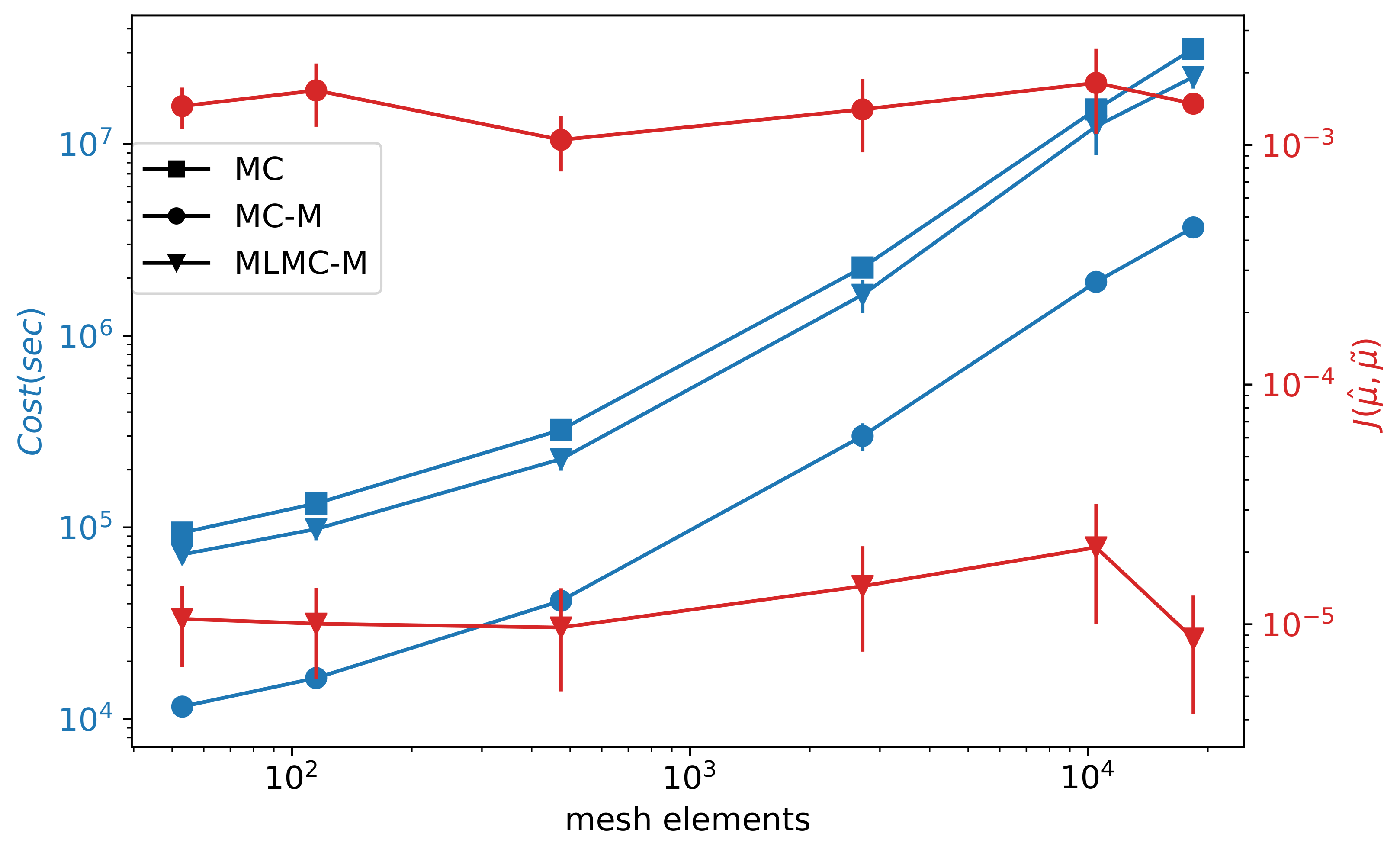
Figure 4 shows the computational cost ( C o s t ( s e c ) ) and moments error ( J ( μ ^ , μ ˜ ) ). The cost is measured as the CPU time of simulations, including auxiliary processing and time needed for meta-model learning. The moments error has the form of MSE: J ( μ ^ , μ ˜ ) = 1 S s = 1 S | | μ ^ s μ ˜ s | | 2 2 , where μ ^ represents the moments estimated by the standard MC, whereas μ ˜ are moments calculated by either MC-M or MLMC-M. As expected, the computational cost increases with the precision of a model expressed as a number of mesh elements. As you can see, the cost can be greatly reduced ( CS 87 % ) by using MC-M instead of MC. However, the meta-model error causes poor estimates of moments: J ( μ ^ , μ ˜ ) 10 3 . On the contrary, MLMC-M suppresses the effect of the meta-model error, and estimates of moments are obtained with J ( μ ^ , μ ˜ ) 10 5 . The cost savings are not so substantial but still significant: CS 25 % . Generally, using MC-M can be reasonable if we have an exceptionally accurate meta-model or we intend to obtain just a basic idea of the moments and PDF in a short time. Otherwise, using the MLMC-M is recommended.

6.3. Multilevel Case

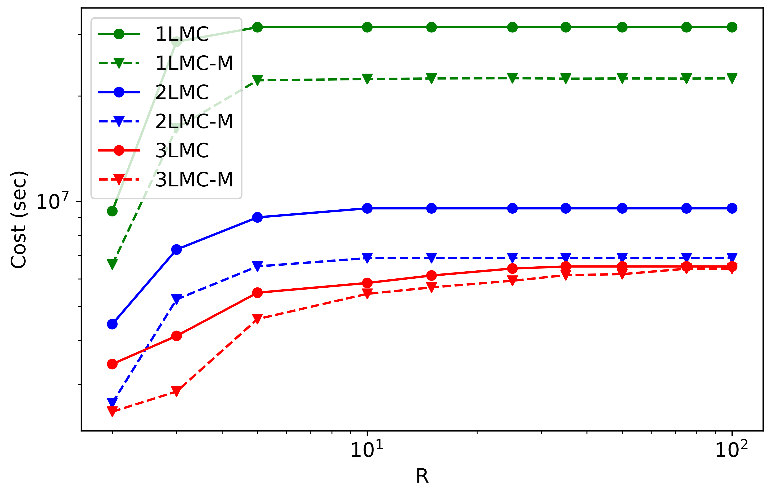
In this section, we investigate an MLMC-M with more than two levels. In order to demonstrate some properties and limitations of our approach, we introduce the following three pairs of Monte Carlo methods:
  • 1LMC and 1LMC-M: standard MC of models on 18,397 mesh elements and its extension by meta-level;
  • 2LMC and 2LMC-M: 2-level MLMC on models with 18,397 and 2714 mesh elements, and its extension by meta-level trained on the model of 2714 mesh elements;
  • 3LMC and 3LMC-M: 3 level MLMC with models on 18,397, 2714, and 474 mesh elements and its extension by meta-level trained on the model of 474 mesh elements
Figure 5 shows the computational costs of these Monte Carlo methods for a different number of estimated moments R. We see that 1LMC and 1LMC-M have a much higher cost than methods with more levels. This is the crucial observation that demonstrates the limitations of the standard MC.
Let us focus on the course of the costs depending on R. In all the cases, the lowest cost was obtained for R = 2 . However, as R increases, the behaviors of the methods differ. For 1LMC, 1LMC-M, 2LMC, and 2LMC-M, we observe a similar course that is steady for R 15 . It means we can add more moments without affecting computational cost. On the other hand, for 3LMC and 3LMC-M, we observe a gradual increase in cost up to R = 35 and R = 75 , respectively.
Regarding computational cost savings, in cases of 1LMC and 2LMC, there is CS 25 % utilizing 1LMC-M and 2LMC-M, whereas 3LMC provides us with savings, from around CS 25 % for R = 2 to just CS 2 % for R = 100 . As mentioned in Section 5.2, the computational cost distribution across levels can be described using β and γ variables. Since for 1LMC and 2LMC, β > γ , the dominant computational cost is on the lowest-accuracy levels. Therefore, adding the meta-level results in a much higher CS (for R > 4 ) than for β < γ , which is the case with 3LMC. Thus, the behavior of our experiments corresponds to the theoretical properties of the MLMC.
A closer look at the variances of moments across levels V ^ l r (Figure 6) provides a rationale for the claims already presented. For clarity, we display only the first five moments ( R = 5 ), which capture the behavior observed also in cases with more moments. To recall, we employ Legendre polynomials as ϕ ( x ) ; therefore, V ^ l 1 = 0 . The total computational cost (see Formula (8)) depends on the number of simulation samples N l that are determined by V ^ l M A X = max { V ^ l r } r = 1 R (see Section 4.1) and C l , which is also displayed in the figure. To meet V t = 10 5 , the pictured variances are calculated based on the following numbers of samples: [ N 1 = 54 , 063 , N 2 = 2550 , N 3 = 1426 ] for 3LMC and [ N 1 = 53 , 342 , N 2 = 36 , 638 , N 3 = 3038 , N 4 = 1218 ] for 3LMC-M.
We can see that V ^ l M A X increases with increasing r for some l, leading to the observed growth of C and C M with R to the point where V ^ l M A X is stable. When it comes to different C S , we need to focus on the course of V ^ l r across levels. We observe increasing V ^ 2 M A X of 3LMC-M, whereas the corresponding V ^ 1 M A X of 3LMC remains constant. This trend is accentuated for R > 5 and causes a decrease in C S . The distinguishable increase in V ^ 1 M A X for 3LMC-M has just a slight impact on C M due to the minor C 1 = 0.338 compared to C l , for l > 1 . A more accurate meta-model could prevent V ^ 2 M A X from increasing for 3LMC-M.
We faced a similar behavior for the groundwater flow problem investigated in our previous research [29]. It is good to be aware of this behavior, although the distribution of variances of moments across MLMC levels would deserve a much more detailed explanation, which is beyond the scope of this article.

6.4. Approximation of Probability Density Function

Finally, we use moments estimated by the cheapest Monte Carlo methods presented (3LMC and 3LMC-M) to approximate the PDF of the contaminant concentration c[kgm 3 ] on the surface, V t = 10 5 , R = 25 . Let ρ 3 L M C , ρ 3 L M C M , ρ M C be the PDFs approximated based on the moments estimated by 3LMC, 3LMC-M, and reference MC. We run N = 50 , 000 model samples on a mesh with 18,397 elements to obtain the reference MC.
Figure 7 depicts the approximated PDFs, as well as the Kullback–Leibler (KL) divergence (for details, see [39]) used for the accuracy assessment of PDFs: D 3 L M C = K L ( ρ r e f | | ρ 3 L M C ) and D 3 L M C M = K L ( ρ r e f | | ρ 3 L M C M ) . Considering the values of V t and R, we have decent PDF approximations. Both 3LMC and 3LMC-M provide almost the same results in terms of KL divergence. It means μ ˜ are sufficiently accurate, in particular J ( μ ^ , μ ˜ ) 8.6 e 6 . Moreover, μ ˜ are obtained with C S 8 % . If we are interested just in the expected value and the variance, which is very common, we have C S 25 % . Importantly, we can decrease V t to obtain a better PDF approximation; in this case, the computational cost naturally increases, but C S does not change.

7. Discussion and Conclusions

This study presented the deep learning meta-model to reduce the computational costs of Monte Carlo methods. We followed up on our previous research [29] and improved the meta-model, which now consists of a graph convolutional neural network connected to the feed-forward neural network. This meta-model can better approximate models such as the tested groundwater contaminant transport problem. We showed that our meta-model could be trained with comparable accuracy for models solved on unstructured meshes from 53 to 18,397 mesh elements.
We adopted Monte Carlo methods to obtain generalized statistical moments that are utilized to approximate the probability density function of the contaminant concentration on the surface above a future deep geological repository of radioactive waste. In order to reduce the computational cost of MC, two approaches were propounded. MC-M, a meta-model instead of a model within the standard Monte Carlo method, brings substantial cost savings ( CS 87 % ). However, the accuracy of moments J was severely affected by the meta-model error and was just around J 10 3 . Under the described experiment setting, it is tough to obtain minor meta-model errors for such a complex model such as the one we have. Thus, this procedure has limited usability. What is favorable, though, is the second approach. A meta-level is employed as the lowest-accuracy level of MLMC, denoted MLMC-M. Generally, this approach reduces the computational cost and keeps the error of moments low, J 10 5 , which is sufficient for PDF approximations. We presented three pairs of MLMCs and MLMC-Ms to demonstrate the impact of a different distribution of computational cost across levels. In accordance with theory, the most significant cost savings ( CS 25 % ) was achieved when the dominant computational cost was on the lowest-accuracy level. On the contrary, if the prevailing computational cost is on the highest-accuracy level, we have CS 2 % in the worst case. Importantly, the computational cost and savings are affected by the number of moments R we estimate. In many applications, we are interested in the first few moments, such as the expected value or the variance. For that, we have CS 25 % in all the cases. Intending to approximate PDF, we need at least around R = 25 , then CS 8 % in the worst-case scenario.
In our future research, we shall try to improve the accuracy of the current meta-model further and investigate the applicability of standard convolutional neural networks as a meta-model. We shall also rigorously describe the causes of the different course of variances of moments across MLMC levels. We shall deal with other applications in groundwater modeling, especially in connection with fractured porous media.

Author Contributions

Conceptualization, M.Š. and J.B.; software, M.Š.; data curation, M.Š.; writing—original draft preparation, M.Š.; writing—review and editing, J.B.; visualization, M.Š.; supervision, J.B.; All authors have read and agreed to the published version of the manuscript.

Funding

This work was supported by the Student Grant Scheme at the Technical University of Liberec through project nr. SGS-2022-3016.

Institutional Review Board Statement

Not applicable.

Informed Consent Statement

Not applicable.

Data Availability Statement

All of the data supporting the findings of the presented study are available from the corresponding author on request.

Acknowledgments

Computational resources were supplied by the project “e-Infrastruktura CZ” (e-INFRA CZ LM2018140) supported by the Ministry of Education, Youth and Sports of the Czech Republic.

Conflicts of Interest

The authors declare no conflict of interest.

Abbreviations

The following abbreviations are used in this manuscript:
DGRdeep geological repository
DNNdeep neural networks
GCNNgraph convolutional neural network
MCMonte Carlo method
MEMMaximum entropy method
MLMCmultilevel Monte Carlo method
NRMSEnormalized mean squared error
PDFprobability density function

References

  1. Fitts, C.R. Groundwater Science, 2nd ed.; Academic Press: Amsterdam, The Netherlands, 2012. [Google Scholar]
  2. Anderson, M.P.; Woessner, W.W.; Hunt, R.J. Applied Groundwater Modeling: Simulation of Flow and Advective Transport, 2nd ed.; Academic Press: Amsterdam, The Netherlands, 2015. [Google Scholar] [CrossRef]
  3. Juckem, P.F.; Fienen, M.N. Simulation of The Probabilistic Plume Extent for a Potential Replacement Wastewater-Infiltration Lagoon, and Probabilistic Contributing Areas for Supply Wells for the Town of Lac Du Flambeau, Vilas County, Wisconsin; Open-File Report; U.S. Geological Survey: Reston, VA, USA, 2020. [CrossRef]
  4. Yoon, H.; Hart, D.B.; McKenna, S.A. Parameter estimation and predictive uncertainty in stochastic inverse modeling of groundwater flow: Comparing null-space Monte Carlo and multiple starting point methods. Water Resour. Res. 2013, 49, 536–553. [Google Scholar] [CrossRef]
  5. Baalousha, H.M. Using Monte Carlo simulation to estimate natural groundwater recharge in Qatar. Model. Earth Syst. Environ. 2016, 2, 1–7. [Google Scholar] [CrossRef] [Green Version]
  6. Giles, M.B. Multilevel Monte Carlo Methods. Acta Numer. 2015, 24, 259–328. [Google Scholar] [CrossRef] [Green Version]
  7. Peherstorfer, B.; Willcox, K.; Gunzburger, M. Survey of Multifidelity Methods in Uncertainty Propagation, Inference, and Optimization. SIAM Rev. 2018, 60, 550–591. [Google Scholar] [CrossRef]
  8. Mohring, J.; Milk, R.; Ngo, A.; Klein, O.; Iliev, O.; Ohlberger, M.; Bastian, P. Uncertainty Quantification for Porous Media Flow Using Multilevel Monte Carlo. In Proceedings of the Large-Scale Scientific Computing, Sozopol, Bulgaria, 8–12 June 2015; Lirkov, I., Margenov, S.D., Waśniewski, J., Eds.; Springer International Publishing: Cham, Switzerland, 2015; pp. 145–152. [Google Scholar]
  9. Iliev, O.; Shegunov, N.; Armyanov, P.; Semerdzhiev, A.; Christov, I. On Parallel MLMC for Stationary Single Phase Flow Problem. In Proceedings of the Large-Scale Scientific Computing, Sozopol, Bulgaria, 7–11 June 2021; Springer International Publishing: Cham, Switzerland, 2022; pp. 464–471. [Google Scholar]
  10. Cliffe, K.A.; Giles, M.B.; Scheichl, R.; Teckentrup, A.L. Multilevel Monte Carlo methods and applications to elliptic PDEs with random coefficients. Comput. Vis. Sci. 2011, 14, 3–15. [Google Scholar] [CrossRef]
  11. Müller, F.; Jenny, P.; Meyer, D.W. Multilevel Monte Carlo for Two Phase Flow and Buckley-Leverett Transport in Random Heterogeneous Porous Media. J. Comput. Phys. 2013, 250, 685–702. [Google Scholar] [CrossRef]
  12. Koziel, S.; Leifsson, L. Surrogate-Based Modeling and Optimization; Springer: New York, NY, USA, 2013. [Google Scholar] [CrossRef]
  13. Asher, M.J.; Croke, B.F.W.; Jakeman, A.J.; Peeters, L.J.M. A review of surrogate models and their application to groundwater modeling. Water Resour. Res. 2015, 51, 5957–5973. [Google Scholar] [CrossRef]
  14. Razavi, S.; Tolson, B.A.; Burn, D.H. Review of surrogate modeling in water resources. Water Resour. Res. 2012, 48, W07401. [Google Scholar] [CrossRef]
  15. Fienen, M.N.; Nolan, B.T.; Feinstein, D.T. Evaluating the sources of water to wells: Three techniques for metamodeling of a groundwater flow model. Environ. Model. Softw. 2016, 77, 95–107. [Google Scholar] [CrossRef]
  16. Hussein, E.A.; Thron, C.; Ghaziasgar, M.; Bagula, A.B.; Vaccari, M. Groundwater Prediction Using Machine-Learning Tools. Algorithms 2020, 13, 300. [Google Scholar] [CrossRef]
  17. Robinson, T.D.; Eldred, M.S.; Willcox, K.E.; Haimes, R. Surrogate-Based Optimization Using Multifidelity Models with Variable Parameterization and Corrected Space Mapping. AIAA J. 2008, 46, 2814–2822. [Google Scholar] [CrossRef] [Green Version]
  18. Jiang, P.; Zhou, Q.; Shao, X. Surrogate Model-Based Engineering Design and Optimization; Springer: Singapore, 2020. [Google Scholar] [CrossRef]
  19. Remesan, R.; Mathew, J. Hydrological Data Driven Modelling; Springer International Publishing: Cham, Switzerland, 2015. [Google Scholar] [CrossRef]
  20. Marçais, J.; de Dreuzy, J.R. Prospective Interest of Deep Learning for Hydrological Inference. Groundwater 2017, 55, 688–692. [Google Scholar] [CrossRef] [PubMed]
  21. Shen, C. A Transdisciplinary Review of Deep Learning Research and Its Relevance for Water Resources Scientists. Water Resour. Res. 2018, 54, 8558–8593. [Google Scholar] [CrossRef]
  22. Yoon, H.; Jun, S.C.; Hyun, Y.; Bae, G.O.; Lee, K.K. A comparative study of artificial neural networks and support vector machines for predicting groundwater levels in a coastal aquifer. J. Hydrol. 2011, 396, 128–138. [Google Scholar] [CrossRef]
  23. Hanoon, M.S.; Ahmed, A.N.; Fai, C.M.; Birima, A.H.; Razzaq, A.; Sherif, M.; Sefelnasr, A.; El-Shafie, A. Application of Artificial Intelligence Models for modeling Water Quality in Groundwater. Water Air Soil Pollut. 2021, 232, 411. [Google Scholar] [CrossRef]
  24. Chen, Y.; Song, L.; Liu, Y.; Yang, L.; Li, D. A Review of the Artificial Neural Network Models for Water Quality Prediction. Appl. Sci. 2020, 10, 5776. [Google Scholar] [CrossRef]
  25. Guezgouz, N.; Boutoutaou, D.; Hani, A. Prediction of groundwater flow in shallow aquifers using artificial neural networks in the northern basins of Algeria. J. Water Clim. Chang. 2020, 12, 1220–1228. [Google Scholar] [CrossRef]
  26. Santos, J.E.; Xu, D.; Jo, H.; Landry, C.; Prodanović, M.; Pyrcz, M.J. PoreFlow-Net: A 3D convolutional neural network to predict fluid flow through porous media. Adv. Water Resour. 2020, 138, 103539. [Google Scholar] [CrossRef]
  27. Yu, X.; Cui, T.; Sreekanth, J.; Mangeon, S.; Doble, R.; Xin, P.; Rassam, D.; Gilfedder, M. Deep learning emulators for groundwater contaminant transport modelling. J. Hydrol. 2020, 590, 125351. [Google Scholar] [CrossRef]
  28. Xu, M.; Song, S.; Sun, X.; Zhang, W. UCNN: A Convolutional Strategy on Unstructured Mesh. arXiv 2021, arXiv:2101.05207. [Google Scholar]
  29. Špetlík, M.; Březina, J. Groundwater flow meta-model for multilevel Monte Carlo methods. In Proceedings of the CEUR Workshop Proceedings, Odesa, Ukraine, 13–19 September 2021; Volume 2962, pp. 104–113. [Google Scholar]
  30. Trudeau, R.J. Introduction to Graph Theory, 1st ed.; Dover Publications: New York, NY, USA, 1993. [Google Scholar]
  31. Hamilton, W.L. Graph Representation Learning. Synth. Lect. Artif. Intell. Mach. Learn. 2020, 14, 1–159. [Google Scholar]
  32. Březina, J.; Stebel, J.; Exner, P.; Hybš, J. Flow123d. 2011–2021. Available online: http://flow123d.github.com (accessed on 19 June 2022).
  33. Goodfellow, I.; Bengio, Y.; Courville, A. Deep Learning; MIT Press: Cambridge, MA, USA, 2016; Available online: http://www.deeplearningbook.org (accessed on 19 June 2022).
  34. Wu, Z.; Pan, S.; Chen, F.; Long, G.; Zhang, C.; Yu, P.S. A Comprehensive Survey on Graph Neural Networks. IEEE Trans. Neural Netw. Learn. Syst. 2021, 32, 4–24. [Google Scholar] [CrossRef] [PubMed] [Green Version]
  35. Defferrard, M.; Bresson, X.; Vandergheynst, P. Convolutional Neural Networks on Graphs with Fast Localized Spectral Filtering. In Proceedings of the Advances in Neural Information Processing Systems, Barcelona, Spain, 5–10 December 2016; Lee, D., Sugiyama, M., Luxburg, U., Guyon, I., Garnett, R., Eds.; Curran Associates, Inc.: Red Hook, NY, USA, 2016; Volume 29. [Google Scholar]
  36. Barron, A.R.; Sheu, C.H. Approximation of Density Functions by Sequences of Exponential Families. Ann. Stat. 1991, 19, 1347–1369. [Google Scholar] [CrossRef]
  37. Březina, J.; Špetlík, M. MLMC Python Library. 2021. Available online: http://github.com/GeoMop/MLMC (accessed on 19 June 2022).
  38. Bierig, C.; Chernov, A. Approximation of probability density functions by the Multilevel Monte Carlo Maximum Entropy method. J. Comput. Phys. 2016, 314, 661–681. [Google Scholar] [CrossRef]
  39. Kullback, S.; Leibler, R.A. On Information and Sufficiency. Ann. Math. Stat. 1951, 22, 79–86. [Google Scholar] [CrossRef]
Figure 1. Contaminant transport problem. A high concentration (X_conc) of a contaminant is spreading from the DGR to the surface. Its course is influenced by the depicted hydraulic conductivity (conductivity) of the rock environment.
Applsci 12 07382 g001
Figure 2. An illustrative example of a random field on an unstructured mesh with the corresponding graph representation.
Applsci 12 07382 g002
Figure 3. Diagram of the architecture of the used deep learning meta-model. The ChebNet graph convolutional neural network is followed by the global summation pool and the deep feed-forward neural network with hidden layers of 64 and 32 neurons. The convolutional kernel has C h channels.
Applsci 12 07382 g003
Figure 4. Cost (blue) and moments error (red) of Monte Carlo methods on six different model mesh sizes. MC (square)—standard Monte Carlo method; MC-M (circle)—standard Monte Carlo using meta-model samples; MLMC-M (triangle)—MC extended by a meta-level. J ( μ ^ , μ ˜ ) denote error between MC moments ( μ ^ ) and MC-M or MLMC-M moments ( μ ˜ ).
Applsci 12 07382 g004
Figure 5. Computational costs of different Monte Carlo methods and number of moments R. XLMC denotes MLMC of X levels, whereas XLMC-M has an additional meta-level.
Applsci 12 07382 g005
Figure 6. Variances of moments across levels for 3LMC (circle) and 3LMC-M (triangle). For legibility, the values are slightly shifted on the x-axis. The leftmost triangles correspond to the meta-level values. The numbers added represent C l [ s e c ] of 3LMC-M.
Applsci 12 07382 g006
Figure 7. PDFs approximated by moments estimated via 3LMC (blue) and 3LMC-M (red dashed). Both compared to the reference MC (black dotted) by the Kullback–Leibler divergence D.
Applsci 12 07382 g007
Table 1. Comparison of accuracy of meta-models for models on different mesh sizes.
Mesh SizeAccuracy of Meta-Model ( J L )
Deep Meta-ModelShallow Meta-Model
53 0.779 0.945
115 0.799 0.949
474 0.763 0.885
2714 0.773 0.896
10,481 0.799 0.898
18,397 0.792 0.954
Publisher’s Note: MDPI stays neutral with regard to jurisdictional claims in published maps and institutional affiliations.

