
Groundwater Contaminant Transport Solved by Monte Carlo Methods Accelerated by Deep Learning Meta-Model


Abstract
:1. Introduction
2. Groundwater Contaminant Transport Model
3. Deep Learning Meta-Model
3.1. Graph Convolutional Neural Network Meta-Model
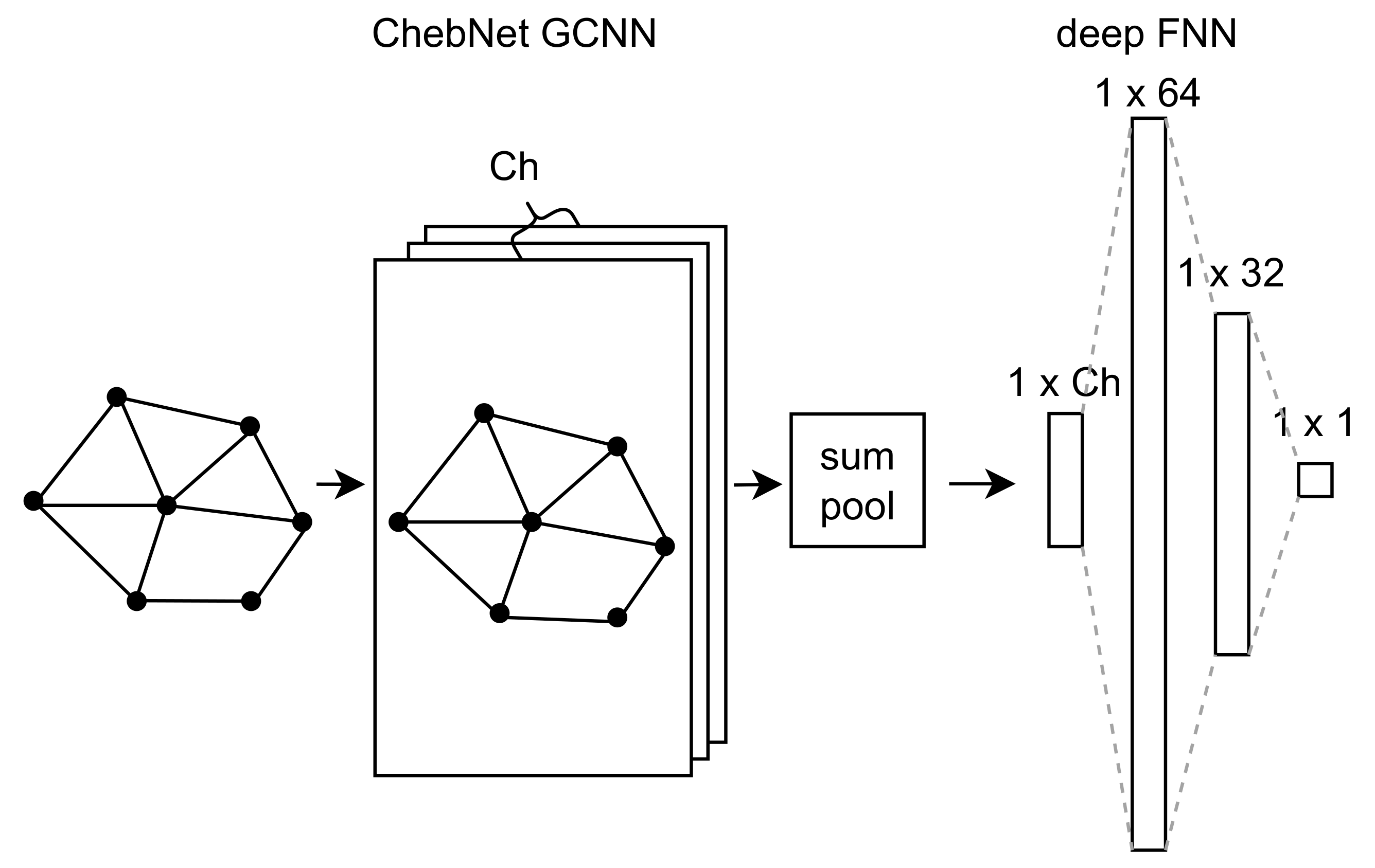
3.2. ChebNet GCNN
3.3. Architecture of Meta-Model
3.4. Assessment of Meta-Model
4. Multilevel Monte Carlo Method
4.1. Optimal Number of Samples
5. Monte Carlo Methods with a Meta-Model
5.1. MC-M
5.2. MLMC-M
6. Results
6.1. Analysis of Meta-Models
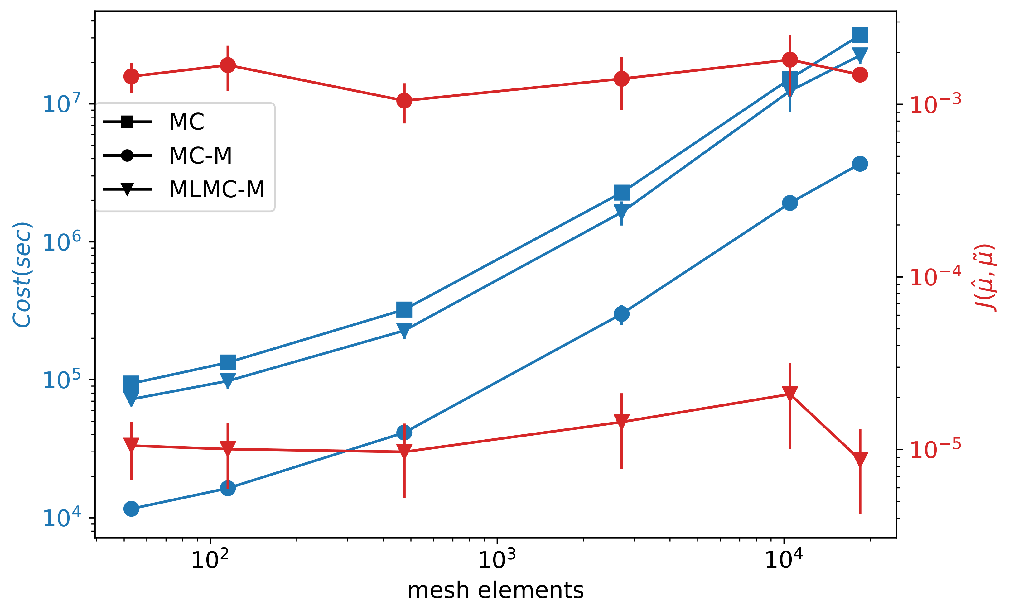
6.2. Comparison of MC-M and MLMC-M
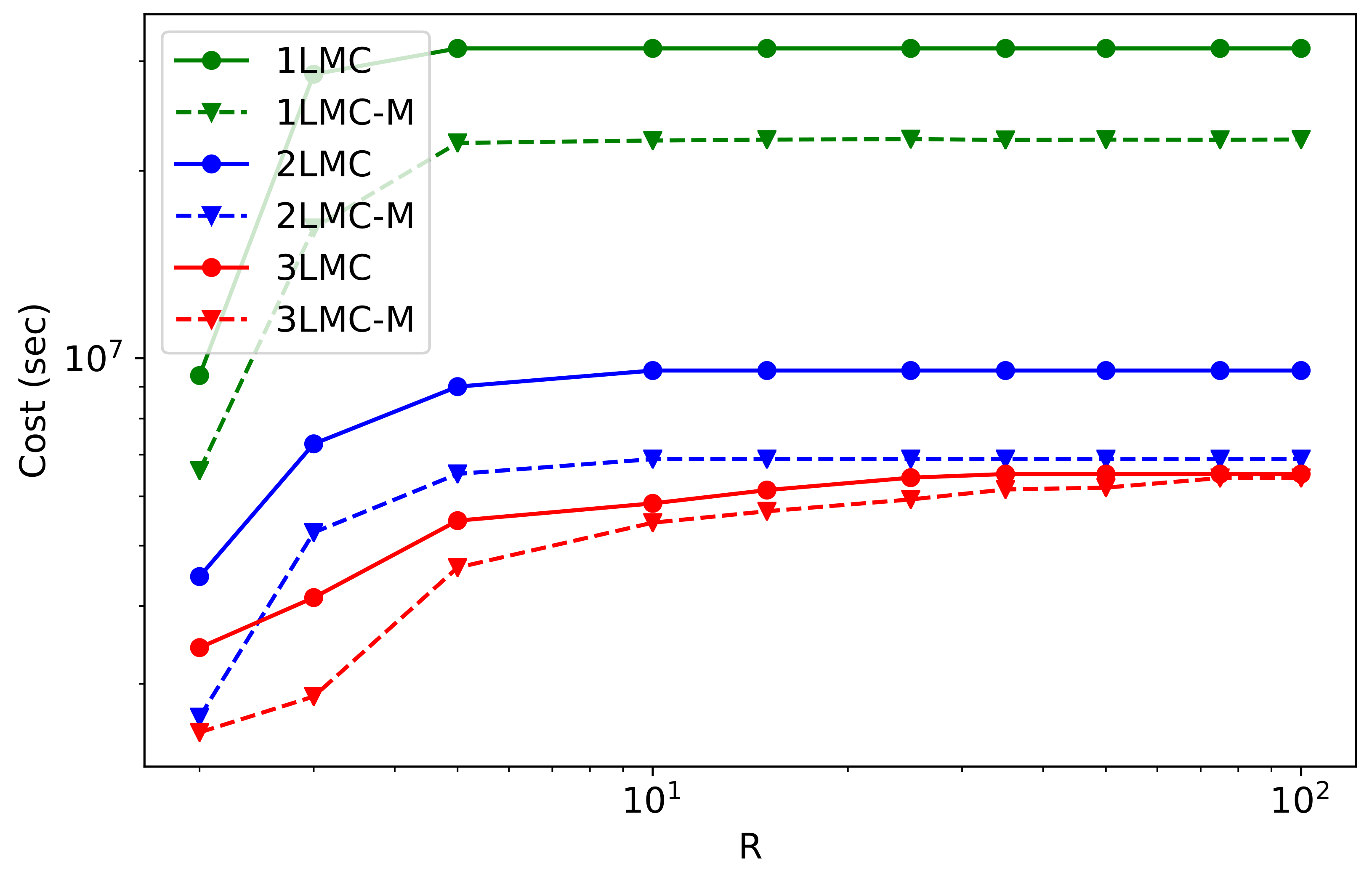
6.3. Multilevel Case
- 1LMC and 1LMC-M: standard MC of models on 18,397 mesh elements and its extension by meta-level;
- 2LMC and 2LMC-M: 2-level MLMC on models with 18,397 and 2714 mesh elements, and its extension by meta-level trained on the model of 2714 mesh elements;
- 3LMC and 3LMC-M: 3 level MLMC with models on 18,397, 2714, and 474 mesh elements and its extension by meta-level trained on the model of 474 mesh elements
6.4. Approximation of Probability Density Function
7. Discussion and Conclusions
Author Contributions
Funding
Institutional Review Board Statement
Informed Consent Statement
Data Availability Statement
Acknowledgments
Conflicts of Interest
Abbreviations
| DGR | deep geological repository |
| DNN | deep neural networks |
| GCNN | graph convolutional neural network |
| MC | Monte Carlo method |
| MEM | Maximum entropy method |
| MLMC | multilevel Monte Carlo method |
| NRMSE | normalized mean squared error |
| probability density function |
References
- Fitts, C.R. Groundwater Science, 2nd ed.; Academic Press: Amsterdam, The Netherlands, 2012. [Google Scholar]
- Anderson, M.P.; Woessner, W.W.; Hunt, R.J. Applied Groundwater Modeling: Simulation of Flow and Advective Transport, 2nd ed.; Academic Press: Amsterdam, The Netherlands, 2015. [Google Scholar] [CrossRef]
- Juckem, P.F.; Fienen, M.N. Simulation of The Probabilistic Plume Extent for a Potential Replacement Wastewater-Infiltration Lagoon, and Probabilistic Contributing Areas for Supply Wells for the Town of Lac Du Flambeau, Vilas County, Wisconsin; Open-File Report; U.S. Geological Survey: Reston, VA, USA, 2020. [CrossRef]
- Yoon, H.; Hart, D.B.; McKenna, S.A. Parameter estimation and predictive uncertainty in stochastic inverse modeling of groundwater flow: Comparing null-space Monte Carlo and multiple starting point methods. Water Resour. Res. 2013, 49, 536–553. [Google Scholar] [CrossRef]
- Baalousha, H.M. Using Monte Carlo simulation to estimate natural groundwater recharge in Qatar. Model. Earth Syst. Environ. 2016, 2, 1–7. [Google Scholar] [CrossRef] [Green Version]
- Giles, M.B. Multilevel Monte Carlo Methods. Acta Numer. 2015, 24, 259–328. [Google Scholar] [CrossRef] [Green Version]
- Peherstorfer, B.; Willcox, K.; Gunzburger, M. Survey of Multifidelity Methods in Uncertainty Propagation, Inference, and Optimization. SIAM Rev. 2018, 60, 550–591. [Google Scholar] [CrossRef]
- Mohring, J.; Milk, R.; Ngo, A.; Klein, O.; Iliev, O.; Ohlberger, M.; Bastian, P. Uncertainty Quantification for Porous Media Flow Using Multilevel Monte Carlo. In Proceedings of the Large-Scale Scientific Computing, Sozopol, Bulgaria, 8–12 June 2015; Lirkov, I., Margenov, S.D., Waśniewski, J., Eds.; Springer International Publishing: Cham, Switzerland, 2015; pp. 145–152. [Google Scholar]
- Iliev, O.; Shegunov, N.; Armyanov, P.; Semerdzhiev, A.; Christov, I. On Parallel MLMC for Stationary Single Phase Flow Problem. In Proceedings of the Large-Scale Scientific Computing, Sozopol, Bulgaria, 7–11 June 2021; Springer International Publishing: Cham, Switzerland, 2022; pp. 464–471. [Google Scholar]
- Cliffe, K.A.; Giles, M.B.; Scheichl, R.; Teckentrup, A.L. Multilevel Monte Carlo methods and applications to elliptic PDEs with random coefficients. Comput. Vis. Sci. 2011, 14, 3–15. [Google Scholar] [CrossRef]
- Müller, F.; Jenny, P.; Meyer, D.W. Multilevel Monte Carlo for Two Phase Flow and Buckley-Leverett Transport in Random Heterogeneous Porous Media. J. Comput. Phys. 2013, 250, 685–702. [Google Scholar] [CrossRef]
- Koziel, S.; Leifsson, L. Surrogate-Based Modeling and Optimization; Springer: New York, NY, USA, 2013. [Google Scholar] [CrossRef]
- Asher, M.J.; Croke, B.F.W.; Jakeman, A.J.; Peeters, L.J.M. A review of surrogate models and their application to groundwater modeling. Water Resour. Res. 2015, 51, 5957–5973. [Google Scholar] [CrossRef]
- Razavi, S.; Tolson, B.A.; Burn, D.H. Review of surrogate modeling in water resources. Water Resour. Res. 2012, 48, W07401. [Google Scholar] [CrossRef]
- Fienen, M.N.; Nolan, B.T.; Feinstein, D.T. Evaluating the sources of water to wells: Three techniques for metamodeling of a groundwater flow model. Environ. Model. Softw. 2016, 77, 95–107. [Google Scholar] [CrossRef]
- Hussein, E.A.; Thron, C.; Ghaziasgar, M.; Bagula, A.B.; Vaccari, M. Groundwater Prediction Using Machine-Learning Tools. Algorithms 2020, 13, 300. [Google Scholar] [CrossRef]
- Robinson, T.D.; Eldred, M.S.; Willcox, K.E.; Haimes, R. Surrogate-Based Optimization Using Multifidelity Models with Variable Parameterization and Corrected Space Mapping. AIAA J. 2008, 46, 2814–2822. [Google Scholar] [CrossRef] [Green Version]
- Jiang, P.; Zhou, Q.; Shao, X. Surrogate Model-Based Engineering Design and Optimization; Springer: Singapore, 2020. [Google Scholar] [CrossRef]
- Remesan, R.; Mathew, J. Hydrological Data Driven Modelling; Springer International Publishing: Cham, Switzerland, 2015. [Google Scholar] [CrossRef]
- Marçais, J.; de Dreuzy, J.R. Prospective Interest of Deep Learning for Hydrological Inference. Groundwater 2017, 55, 688–692. [Google Scholar] [CrossRef] [PubMed]
- Shen, C. A Transdisciplinary Review of Deep Learning Research and Its Relevance for Water Resources Scientists. Water Resour. Res. 2018, 54, 8558–8593. [Google Scholar] [CrossRef]
- Yoon, H.; Jun, S.C.; Hyun, Y.; Bae, G.O.; Lee, K.K. A comparative study of artificial neural networks and support vector machines for predicting groundwater levels in a coastal aquifer. J. Hydrol. 2011, 396, 128–138. [Google Scholar] [CrossRef]
- Hanoon, M.S.; Ahmed, A.N.; Fai, C.M.; Birima, A.H.; Razzaq, A.; Sherif, M.; Sefelnasr, A.; El-Shafie, A. Application of Artificial Intelligence Models for modeling Water Quality in Groundwater. Water Air Soil Pollut. 2021, 232, 411. [Google Scholar] [CrossRef]
- Chen, Y.; Song, L.; Liu, Y.; Yang, L.; Li, D. A Review of the Artificial Neural Network Models for Water Quality Prediction. Appl. Sci. 2020, 10, 5776. [Google Scholar] [CrossRef]
- Guezgouz, N.; Boutoutaou, D.; Hani, A. Prediction of groundwater flow in shallow aquifers using artificial neural networks in the northern basins of Algeria. J. Water Clim. Chang. 2020, 12, 1220–1228. [Google Scholar] [CrossRef]
- Santos, J.E.; Xu, D.; Jo, H.; Landry, C.; Prodanović, M.; Pyrcz, M.J. PoreFlow-Net: A 3D convolutional neural network to predict fluid flow through porous media. Adv. Water Resour. 2020, 138, 103539. [Google Scholar] [CrossRef]
- Yu, X.; Cui, T.; Sreekanth, J.; Mangeon, S.; Doble, R.; Xin, P.; Rassam, D.; Gilfedder, M. Deep learning emulators for groundwater contaminant transport modelling. J. Hydrol. 2020, 590, 125351. [Google Scholar] [CrossRef]
- Xu, M.; Song, S.; Sun, X.; Zhang, W. UCNN: A Convolutional Strategy on Unstructured Mesh. arXiv 2021, arXiv:2101.05207. [Google Scholar]
- Špetlík, M.; Březina, J. Groundwater flow meta-model for multilevel Monte Carlo methods. In Proceedings of the CEUR Workshop Proceedings, Odesa, Ukraine, 13–19 September 2021; Volume 2962, pp. 104–113. [Google Scholar]
- Trudeau, R.J. Introduction to Graph Theory, 1st ed.; Dover Publications: New York, NY, USA, 1993. [Google Scholar]
- Hamilton, W.L. Graph Representation Learning. Synth. Lect. Artif. Intell. Mach. Learn. 2020, 14, 1–159. [Google Scholar]
- Březina, J.; Stebel, J.; Exner, P.; Hybš, J. Flow123d. 2011–2021. Available online: http://flow123d.github.com (accessed on 19 June 2022).
- Goodfellow, I.; Bengio, Y.; Courville, A. Deep Learning; MIT Press: Cambridge, MA, USA, 2016; Available online: http://www.deeplearningbook.org (accessed on 19 June 2022).
- Wu, Z.; Pan, S.; Chen, F.; Long, G.; Zhang, C.; Yu, P.S. A Comprehensive Survey on Graph Neural Networks. IEEE Trans. Neural Netw. Learn. Syst. 2021, 32, 4–24. [Google Scholar] [CrossRef] [PubMed] [Green Version]
- Defferrard, M.; Bresson, X.; Vandergheynst, P. Convolutional Neural Networks on Graphs with Fast Localized Spectral Filtering. In Proceedings of the Advances in Neural Information Processing Systems, Barcelona, Spain, 5–10 December 2016; Lee, D., Sugiyama, M., Luxburg, U., Guyon, I., Garnett, R., Eds.; Curran Associates, Inc.: Red Hook, NY, USA, 2016; Volume 29. [Google Scholar]
- Barron, A.R.; Sheu, C.H. Approximation of Density Functions by Sequences of Exponential Families. Ann. Stat. 1991, 19, 1347–1369. [Google Scholar] [CrossRef]
- Březina, J.; Špetlík, M. MLMC Python Library. 2021. Available online: http://github.com/GeoMop/MLMC (accessed on 19 June 2022).
- Bierig, C.; Chernov, A. Approximation of probability density functions by the Multilevel Monte Carlo Maximum Entropy method. J. Comput. Phys. 2016, 314, 661–681. [Google Scholar] [CrossRef]
- Kullback, S.; Leibler, R.A. On Information and Sufficiency. Ann. Math. Stat. 1951, 22, 79–86. [Google Scholar] [CrossRef]


| Mesh Size | Accuracy of Meta-Model () | |
|---|---|---|
| Deep Meta-Model | Shallow Meta-Model | |
| 53 | ||
| 115 | ||
| 474 | ||
| 2714 | ||
| 10,481 | ||
| 18,397 | ||
Publisher’s Note: MDPI stays neutral with regard to jurisdictional claims in published maps and institutional affiliations. |
© 2022 by the authors. Licensee MDPI, Basel, Switzerland. This article is an open access article distributed under the terms and conditions of the Creative Commons Attribution (CC BY) license (https://creativecommons.org/licenses/by/4.0/).
Share and Cite
Špetlík, M.; Březina, J. Groundwater Contaminant Transport Solved by Monte Carlo Methods Accelerated by Deep Learning Meta-Model. Appl. Sci. 2022, 12, 7382. https://doi.org/10.3390/app12157382
Špetlík M, Březina J. Groundwater Contaminant Transport Solved by Monte Carlo Methods Accelerated by Deep Learning Meta-Model. Applied Sciences. 2022; 12(15):7382. https://doi.org/10.3390/app12157382
Chicago/Turabian StyleŠpetlík, Martin, and Jan Březina. 2022. "Groundwater Contaminant Transport Solved by Monte Carlo Methods Accelerated by Deep Learning Meta-Model" Applied Sciences 12, no. 15: 7382. https://doi.org/10.3390/app12157382
APA StyleŠpetlík, M., & Březina, J. (2022). Groundwater Contaminant Transport Solved by Monte Carlo Methods Accelerated by Deep Learning Meta-Model. Applied Sciences, 12(15), 7382. https://doi.org/10.3390/app12157382