Abstract
The future motion prediction of vehicles in the front is widely valued for its great potential to improve a vehicle’s safety, fuel consumption, and efficiency. However, due to the uncertainty of a driver’s driving intentions and vehicle dynamics, future motion prediction faces great challenges. In order to break the bottleneck in the prediction of leading vehicle motion, this paper proposes a prediction idea of decoupling the prediction of leading vehicle motion into vertical vehicle speed prediction based on the Gaussian process regression algorithm and horizontal heading angle prediction based on the long short-term memory method, which combines the predicted vehicle speed and heading angle to derive the future trajectory of the leading vehicle. Moreover, we propose a prediction algorithm of the leading vehicle motion based on the combination of driving intention recognition and multimodel prediction results by the Fuzzy C-means algorithm, which tries to solve the problem of the unclear driving intention of the predicted object and the nonlinearity between the future motion of the vehicle and the environment. Finally, the algorithm is validated using real vehicle data, proving that it has high prediction accuracy.
1. Introduction
The future driving actions of the leading vehicle have a considerable influence on the operation behavior of the vehicle, which in turn affects the fuel consumption, driving security, and transportation efficiency of the vehicle, especially in the lane change, overtaking, and ramp merging scenarios. However, there are limited data collection sources related to the front car’s trajectory. Therefore, the dynamics of the front car cannot be accurately calculated, thus affecting the accuracy of the front car’s action prediction. In addition, there is uncertainty about the driving intention of the leading vehicle. Finally, the trajectory prediction should not only predict the future coordinate points of the vehicle but also focus on the vehicle’s future heading angle and the leading vehicle’s future speed.
As a result, the trajectory forecasting of major vehicles is challenged by uncertainties about a driver’s driving intentions and dynamics and limited data sources.
Therefore, the accuracy of the trajectory prediction of the front vehicle is largely influenced by the uncertainty of the driving intention and dynamics of the leading vehicle. Current vehicle trajectory prediction methods are mainly divided into maneuver-based models and end-to-end models [1,2,3]. Xie [4] considered kinematic models in a physics-based prediction model. Deo [5] designed a trajectory prediction module based on the amalgamation of an interacting multiple model (IMM) based motion model and maneuver-specific variational Gaussian mixture models (VGMMs). The performance of the model-based parameterization method is influenced by the accuracy of the kinetic properties of the object [6]. The method has strong environmental adaptability. However, with limited data sources, it is impossible to build complex vehicle behavior models to describe factors, including road structure and traffic rules, and derive complex trajectory prediction algorithms.
Historical data-driven parameterization is mainly used in model training to understand the nonlinear relation between prediction and output. For example, Ballan [7] learns scene-specific motion patterns based on the shroom role between the state of moving objects and the semantic information of the scene and applies them to new scenes featuring similar elements for motion prediction. Ye [8] performs vehicle trajectory prediction based on a hidden Markov model with parameters determined from historical trajectory data. The authors of [9] proposed a recurrent neural network model for urban vehicle trajectory prediction based on attention mechanism. In [10], LSTM (long short-term memory) is used to learn the mapping from the input of the original sensor to the object coordinates in an unsupervised manner. In [11], the sequence of vehicle coordinates obtained from sensor measurements is fed to the LSTM, and probabilistic information about the future location of the vehicle on the occupancy grid map is generated. Choi et al. [12] proposed a trajectory prediction method based on a random forest (RF) algorithm and a long short-term memory (LSTM) encoder–decoder architecture. Shen et al. [13] based their process on visual recognition of lane lines and vehicles and input the vehicle coordinate sequence into the LSTM algorithm to predict the future coordinates of the target vehicle. These methods do not take into account the driver’s driving intention but only focus on the future trajectory points of the car in front of it and do not predict or modify future speeds by default.
Because it is difficult to detect driving intentions directly through sensors, Liu et al. [14] developed a driving behavior estimation-based model that uses a hidden Markov model to classify whether a vehicle makes a lane change or not. Gindele et al. [15] proposed a dynamic Bayesian network-based filter that estimates whether future vehicles have acceleration, deceleration, and overtaking operations and predicts future trajectories based on current driver decision behavior. Rákos et al. [16] used variational autoencoder (VAE) to classify driving intentions into lane-keeping, left turn, and right turn. Woo et al. [17] used the SVM algorithm to classify driving intentions into keeping, changing, arrival, and adjustment. Yuan et al. [18] developed a prediction method for lane change maneuvers of the vehicle in front using a hidden Markov model based on the distance between the primary vehicle and the vehicle in front and the lateral and longitudinal speed of the vehicle in front. Han et al. [19] predicted the vehicle lane change left (LCL), lane change right (LCR), and lane-keeping (LK) predictions based on the LSTM algorithm and selected the behavior with the highest probability from them as the future the driving behavior. However, most methods classify lane-changing operations, lane-keeping, and vertical driving intentions as aggressive and moderate [20], with low classification accuracy, and do not accurately describe the lane-changing process [21,22,23]. Instead of outputting discrete values, the classification results of the FCM algorithm output the probabilities belonging to different outcomes, which can improve the resolution and classification accuracy of the classification results, thus avoiding overly aggressive or conservative results of the prediction model. For example, Wang et al. [24] used acceleration and deceleration behavior, overspeed behavior, and operational stability as feature parameters to classify driver driving behavior using the FCM clustering method. Liu et al. [25] used speed, acceleration, and gas pedal opening as feature quantities for the FCM algorithm to classify driving styles.
According to the uncertainty of driving behavior and vehicle dynamics characteristics, this paper decomposes the problem of driving behavior recognition prediction into vertical speed prediction and horizontal heading angle prediction. The FCM method was applied to classify driving intentions to improve the accuracy and resolution of driving behavior pattern recognition. The model is trained with real vehicle data for different driving intentions. To accurately predict the future actions of the leading car, the action prediction is decoupled into vertical velocity prediction and horizontal heading angle prediction instead of just predicting coordinate points. For the horizontal prediction problem, the LSTM algorithm is used to predict the heading angle of the leading car, and for the vertical prediction problem, the GPR algorithm is used to predict the speed of the leading car and combine it with the calculated future trajectory. Finally, real vehicle data are used to validate the algorithm proposed.
The rest of this article is arranged as follows. Section 2 describes the proposed trajectory prediction model, including the principle of the algorithm and the framework of the trajectory prediction algorithm. Section 3 introduces the research object and evaluation criteria and analyzes the experimental results, and Section 4 concludes the paper.
2. Methods
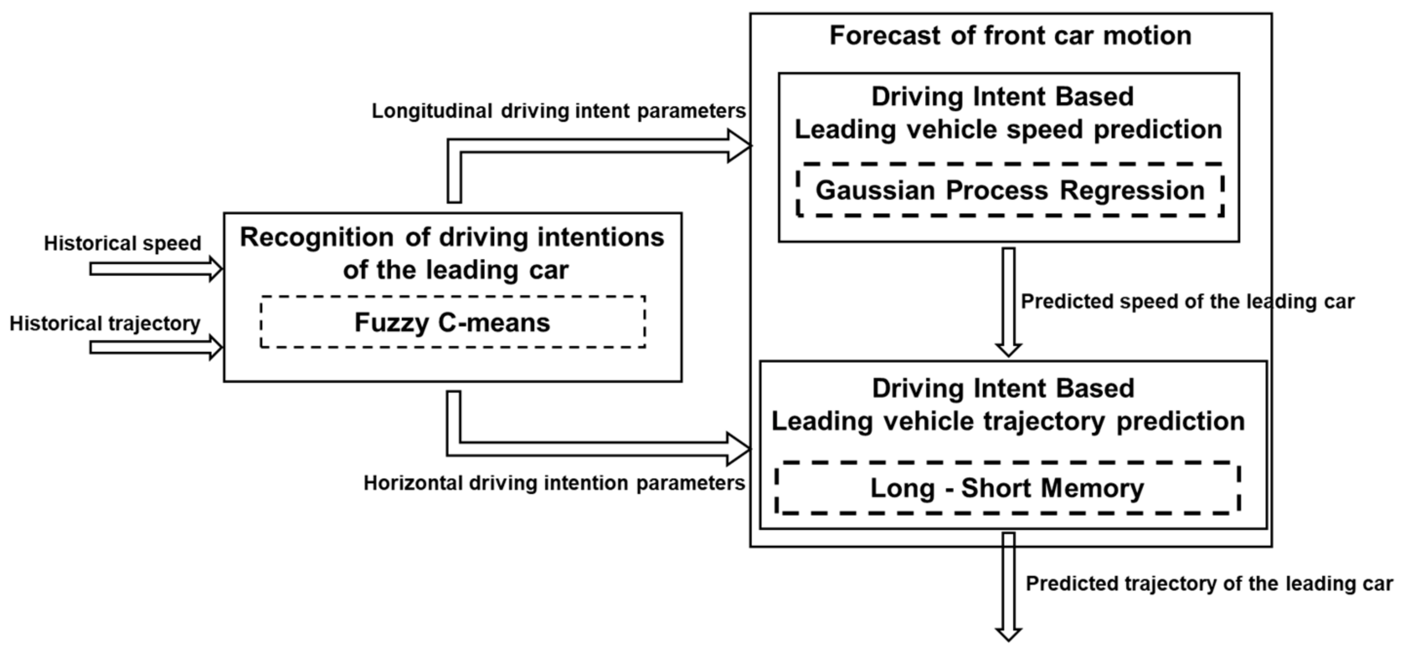
For the problem of predicting the future motion of the front vehicle, there is the problem of unclear driving intention and dynamics characteristics of the front vehicle, and the following ideas are proposed in this paper. First, for the problem of the unclear driving intention of the front vehicle, the driving intention is divided into vertical driving intention and horizontal driving intention, and FCM is used to extract the corresponding feature parameters by using vehicle acceleration and trajectory-related information; the driving intention is then automatically recognized through offline training. Secondly, the leading vehicle motion prediction problem is decomposed into vertical speed prediction and horizontal heading angle prediction. The GPR and LSTM methods are used to predict future vehicle speeds and heading angles using historical and current vehicle speeds and coordinate information combined with weight coefficients of different driving intentions. Then, based on the classification results of different driving intentions, three predicted speeds and heading angles are fused, and the 1s rolling prediction is made using an iterative method. Finally, the predicted vehicle speed and heading angle are combined to calculate the final vehicle trajectory. The structure diagram of the forward vehicle trajectory prediction algorithm is shown in Figure 1.

Figure 1.
Structure of the leading vehicle motion prediction algorithm.
2.1. Driving Intent Classification
In general, drivers need to turn on their turn signals in the appropriate direction before making a lane change operation. However, statistics [26] show that turn signals were used in only 78.6 percent of lane changes, and that some drivers turned on their signals after the lane change began rather than during the initial phase, with less than 50 percent of drivers turning on their signals during the initial phase. Therefore, it is not enough to use turn signals to identify driving intentions, and other characteristic parameters are also needed to distinguish driving intentions.
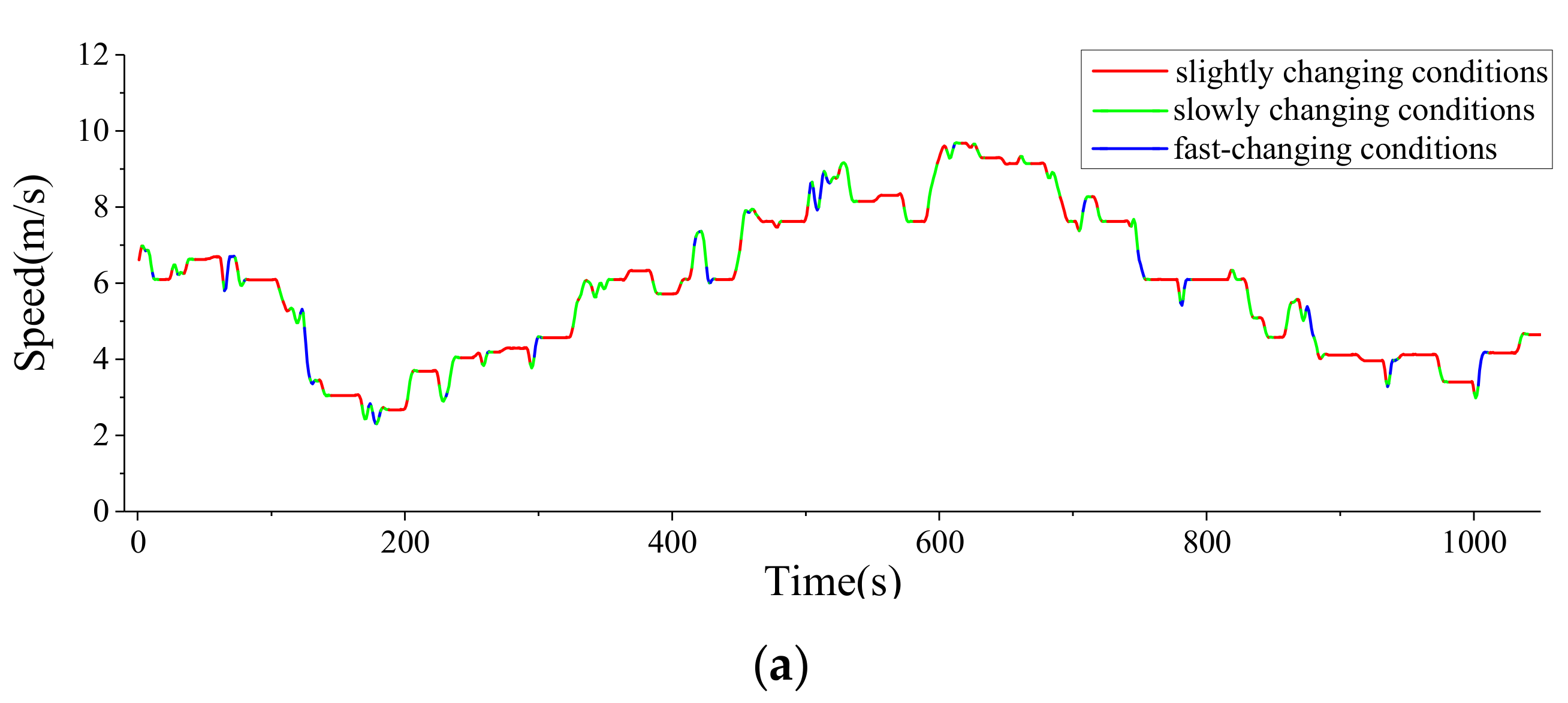
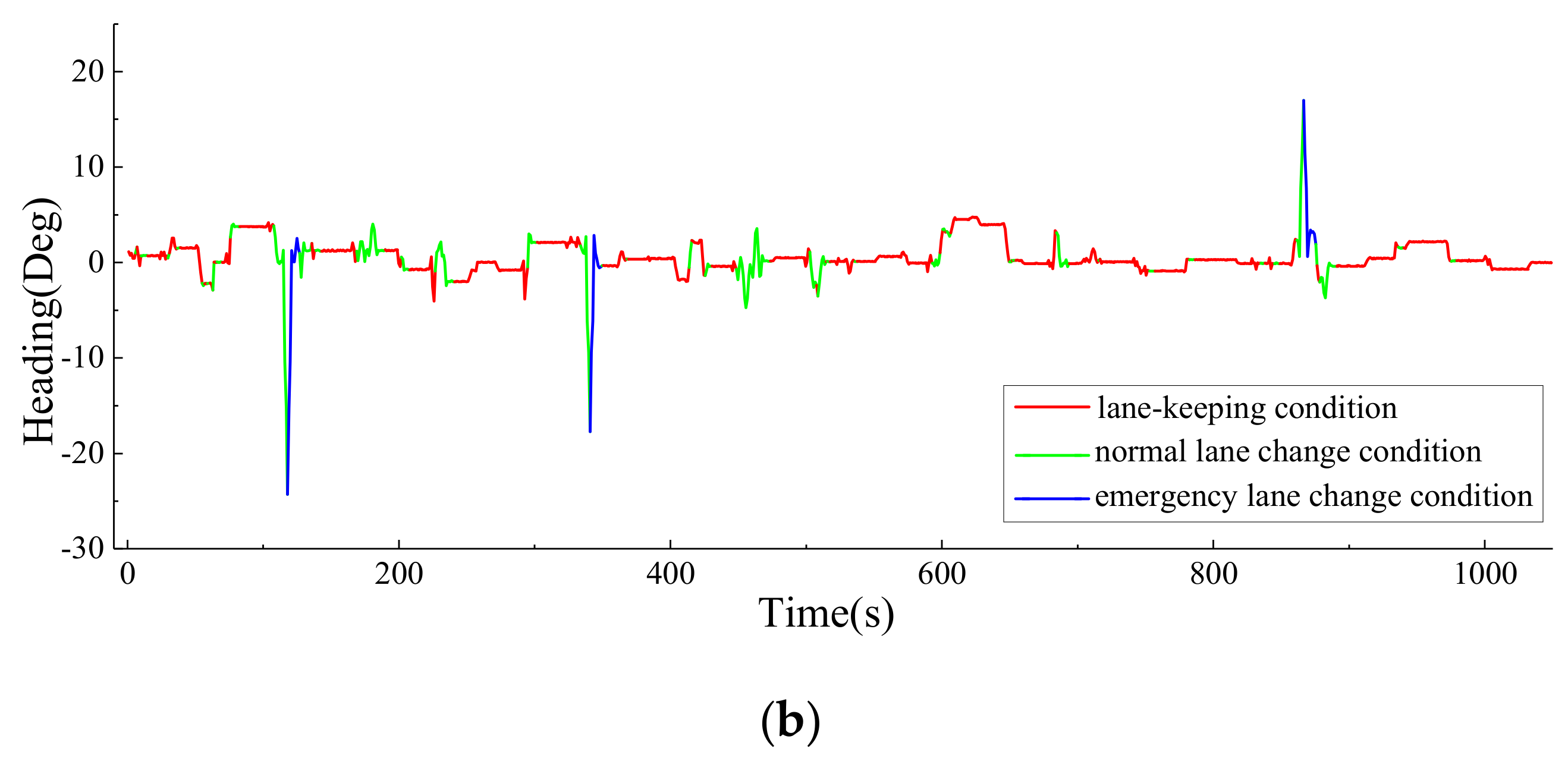
We classified vertical driving intentions into slightly changing, slowly, and fast-changing conditions. The horizontal driving intent is classified into lane-keeping conditions, normal lane change conditions, and emergency lane change conditions. The probability of belonging to each driving intention in the future is identified to improve the accuracy and resolution of the identification, and the identification results are used as weighting factors for the predicted vehicle speed and heading angle fusion module.
In order to distinguish between vertical and horizontal driving intentions, the corresponding feature parameters are extracted for classifying driving intentions in the horizontal and vertical directions, respectively. Table 1 and Table 2 show the selected feature parameters.

Table 1.
Table of horizontal characteristic parameters.
Table 2.
Table of vertical characteristic parameters.
A portion of the real vehicle data is selected as the training set, and the historical 4-step and current moment data are composed as a set. The extracted feature parameters of each set are used as the input of the FCM algorithm, and the clustering center and affiliation matrix are updated until the conditions of the objective function are satisfied. The final degree of similarity between data of the same category is maximized.
The FCM algorithm is applied to determine the clustering center and affiliation matrix. Before satisfying the objective function shown in Equation (1), the clustering centers and affiliation functions are iterated according to Equations (2) and (3) to obtain the clustering centers for lane-keeping condition , normal lane change condition , and emergency lane change condition in the horizontal direction, and the clustering centers for slightly changing conditions , slowly changing conditions and fast-changing conditions in the vertical direction.
where is the objective function, denotes the cluster center of class j, denotes the affiliation of the sample belonging to class s, and for a single sample , the sum of the affiliation for each class is 1.
In order to solve the problem of driving intention classification, the current and historical 4-step sampling time data are used as a group in the process of actual vehicle driving, and the feature values of this group are extracted. Furthermore, the distance from the current moment data to each cluster center and the respective affiliation function are calculated using Equation (3), which represents the probability of its belonging to that cluster center.
2.2. Speed Prediction
Gaussian Process Regression (GPR) methods have shown great potential in dealing with the uncertain relationship between inputs and outputs compared to existing popular nonparametric forecasting methods such as neural networks [27,28]. In [29], the results showed that traffic flow prediction using Gaussian models outperformed the commonly used methods. In [30], a conditional linear Gaussian model is proposed for multistep prediction of leading velocity, and the model is trained to estimate the probability distribution of leading velocity using actual measurement data. Authors of [31] developed a multistep Gaussian process regression model to predict the driver’s future power demand using vehicle–vehicle and vehicle–road information. Authors of [32] used a Gaussian process approach to estimate future vehicle motion from vehicle-to-vehicle and vehicle-to-infrastructure information. However, the above papers require the use of a priori roadwork information in vehicle speed prediction. Because the vehicle-to-vehicle information can be obtained without identifying the driving intention of the previous vehicle, the accurate prediction of the speed of the previous vehicle cannot be made when the data sources are limited, especially when the vehicle-to-road information and vehicle-to-vehicle information are not available, but there is room for further improvement.
GPR considers f(x) to be related to some specific models compared to Gaussian processes, which can represent f(x) indirectly but rigorously by allowing the data to represent the input–output relationship of the object. Gaussian process regression is a form of supervised learning method with fewer parameters.
GPs extend multivariate Gaussian distributions to an infinite number of dimensions. Formally Gaussian processes distribute the data in regions where any finite subset follows a multivariate Gaussian distribution. For all , which obey a multivariate Gaussian distribution, f is said to be a Gaussian process, denoted as:
where is the mean value function and is the covariance matrix.
The Gaussian noise model is used to represent the measured and noise values during data observation, which means:
where x is the vector of independent variables, i.e., the eigenvector. assumes that there is a Gaussian process prior to this, which means:
The effect of noise is also introduced in the covariance function, as in Equation (7):
where is the maximum covariance, and and are the hyperparameters determined during model training using the maximum likelihood estimation method. The covariance function can be understood as a measure of similarity between two x. is Kronecker delta function, whose independent variables are usually two integers, and its output value is 1 if they are equal, otherwise it is 0.
With the covariance function, the covariance matrix is calculated for all input observations as in Equation (8):
For the new point , the covariance matrix corresponding to the point is
The Gaussian process defines the joint distribution as a Gaussian distribution, then the corresponding prior distributions for the training set output and the test point output are shown in Equation (11):
The posterior probability distribution and best estimate of is calculated as shown in Equations (12) and (13):
The actual speed data with different driving intentions, five steps of historical data as input, and 1 step of future speed data as output are used to train the GPR model separately to form the GPR speed predictor for different driving intentions, respectively.
The GPR model takes the speed data of 5 historical sampling steps as input, and the results of the FCM-based driving intention classification introduced in the previous section are used as the result weights of each GPR model to finally predict the speed of the future 1 step.
2.3. Trajectory Prediction
Recurrent neural networks (RNNs) are widely used to analyze the time-series data structure. The long short-term memory (LSTM) model is a variant of RNN that learns long-term dependent information, and the main difference between the long short-term memory network and the traditional recurrent neural network is its added gate structure, which is input gate, forgetting gate, and output gate [33]. The relevant formula for the LSTM is:
where denotes the forgetting gate, denotes the input gate, denotes the state update, denotes the output gate, and denotes the final output value. , , , , , , , denotes the weight coefficient; , , , denotes the bias; and is the activation function.
First, three LSTM algorithm models were trained using data from different driving intentions, with the historical 4-step length and current heading angles as inputs and the future 1-step heading angle as output. Then the probability of three lane change patterns is determined by combining the FCM algorithm, the future heading angle of the three LSTMs deviation model is obtained with multimodel fusion, and the future vehicle position is calculated with Equations (22) and (23) based on the current speed of the vehicle.
2.4. Multistep Prediction
Currently, multistep prediction tasks can be performed either by explicitly training a direct model to predict the overstep, called the direct method, or by repeating the one-step overstep prediction until the desired horizon, called the iterative method [34]. The results show that the direct method requires a much higher training data volume and computational effort than the iterative method [35,36]. In this paper, the prediction of speed and trajectory is chosen for the iterative method; furthermore, to reduce the cumulative error caused by the iterative method, the driving intention is identified for each prediction step.
As an example of predicting a future 2-step trajectory, with the input data of historical 3-step and current moment trajectory information, as well as predicted future 1-step trajectory information, after extracting the corresponding feature parameters, the probability that the set of data belongs to different driving intentions is identified by the FCM algorithm. The trajectory data and the probability of driving intention data are input in the LSTM trajectory predictor, and the driving intention probability data are used as weight parameters, which are combined with the trajectory prediction results calculated based on different driving intentions to finally predict the car’s trajectory ahead of the next two steps.
3. Experimental Results and Analysis
3.1. Research Subjects
The research object of this paper is a purely electric bus, with the configuration parameters shown in Table 3.
Table 3.
Table of electric bus parameters configuration.
The data for this study were obtained from the millimeter-wave radar loaded on the vehicle and mounted at the vehicle’s front windshield. The collected vehicle data , where each data set in C is the speed and relative position information of the leading vehicle in the horizontal and vertical directions. The data cover a wide range of operating conditions and are collected at a frequency of 100 ms. The dataset includes different operating conditions, including uniform speed, acceleration, rapid acceleration, deceleration, rapid deceleration, lane change, and abrupt lane change, covering different vehicle behaviors, and is used to simulate vehicle conditions under different operating conditions in order to improve the algorithm’s ability to adapt in different environments. The collected data are divided into training, validation, and test sets, which train, validate, and test the driver intention classification algorithm and prediction algorithm.
3.2. Evaluation Indicators
In this paper, root mean square error (RMSE) and mean absolute error (MAE) were chosen as the indicators to evaluate the accuracy of trajectory prediction. Among them, RMSE measures deviations between predictions and real values and is more sensitive to outliers in data. MAE represents the average of absolute errors between predictions and observations, denoted as:
where m is the number of samples, is the predicted result, and is the real operating data of the vehicle.
3.3. Experimental Results Analysis
In the driving intention classification, 20 groups of vehicle operation data, totaling 20,238 sample points, were randomly selected for testing. The average recognition accuracy of vertical driving intention is 94.83%, and the average recognition accuracy of horizontal driving intention is 93.25%, which has a good recognition effect on driving intention. Figure 2 shows the driving intention classification results from one set of vehicle data, with different colors representing different driving intentions in the horizontal and vertical directions.
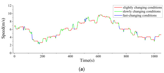
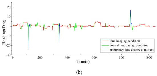
Figure 2.
Driving intent classification results: (a) vertical driving intention classification results; (b) horizontal driving intention classification results.
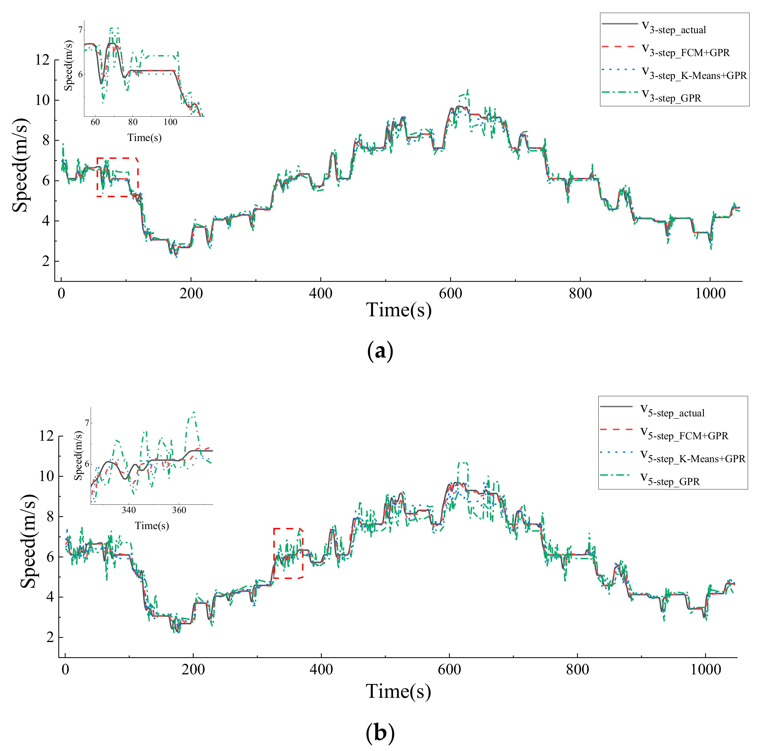
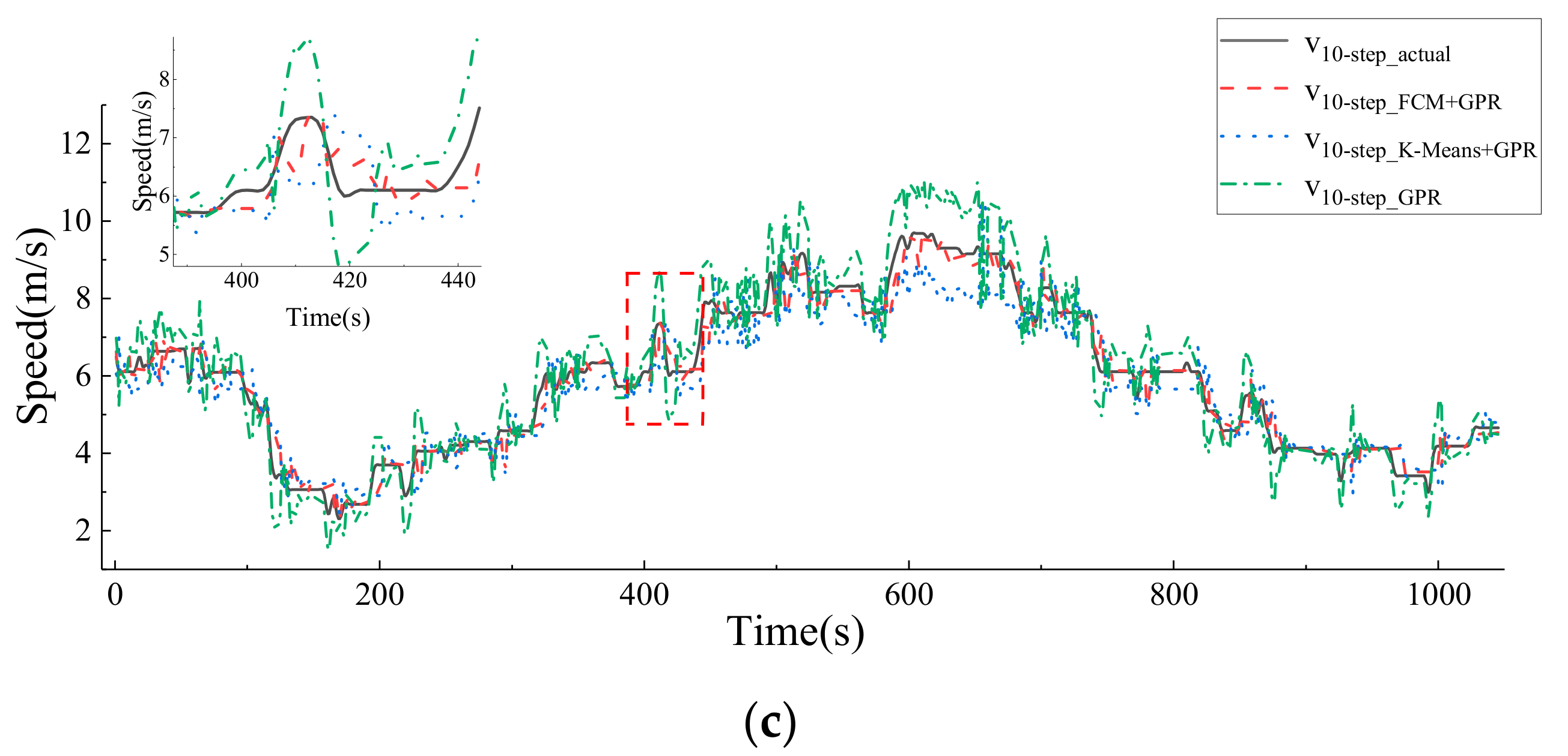
The results of the multistep prediction of future velocity using the iterative method are shown in Figure 3, and the graphs show the comparison curves of velocity prediction results for the third, fifth, and tenth steps of the prediction. From the figure, it can be seen that the error of velocity prediction increases with the increase in the prediction step length. Secondly, in the case of drastic speed changes, the other two methods have more aggressive prediction results than the algorithm used in this paper, and the difference is more obvious in the case of frequent acceleration and deceleration. The GPR prediction curve based on FCM is closer to the real speed of the vehicle in front, and the prediction error is significantly reduced.
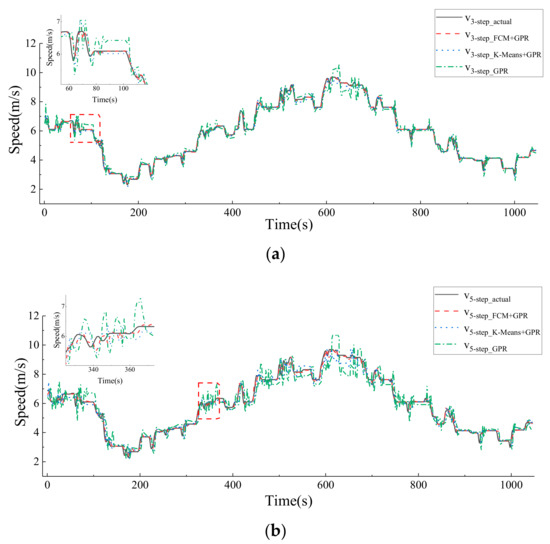
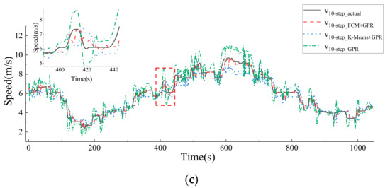
Figure 3.
Comparison of multistep velocity prediction results: (a) comparison of the results of 3-step speed prediction; (b) comparison of the results of 5-step speed prediction; (c) comparison of the results of 10-step speed prediction.
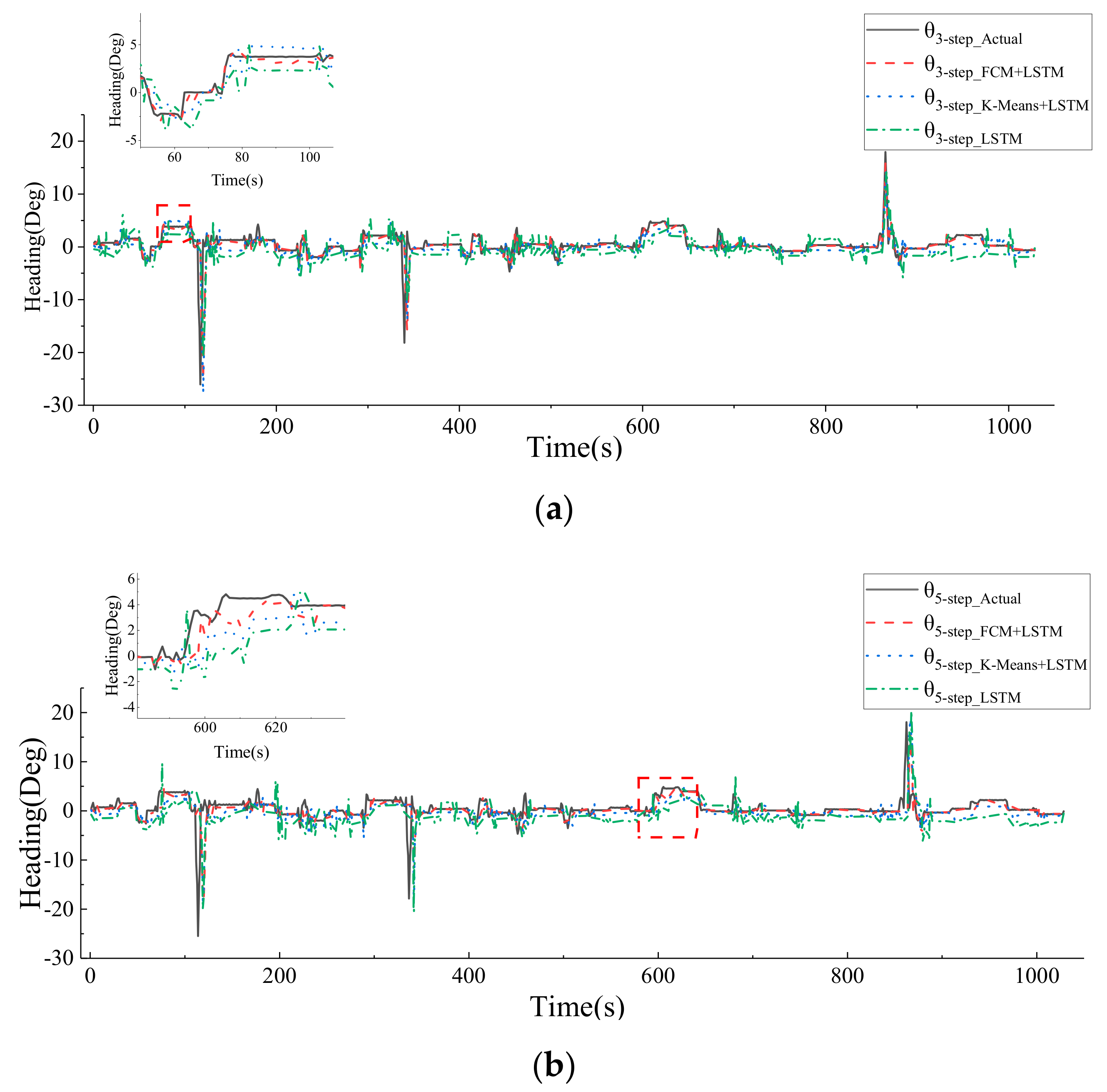
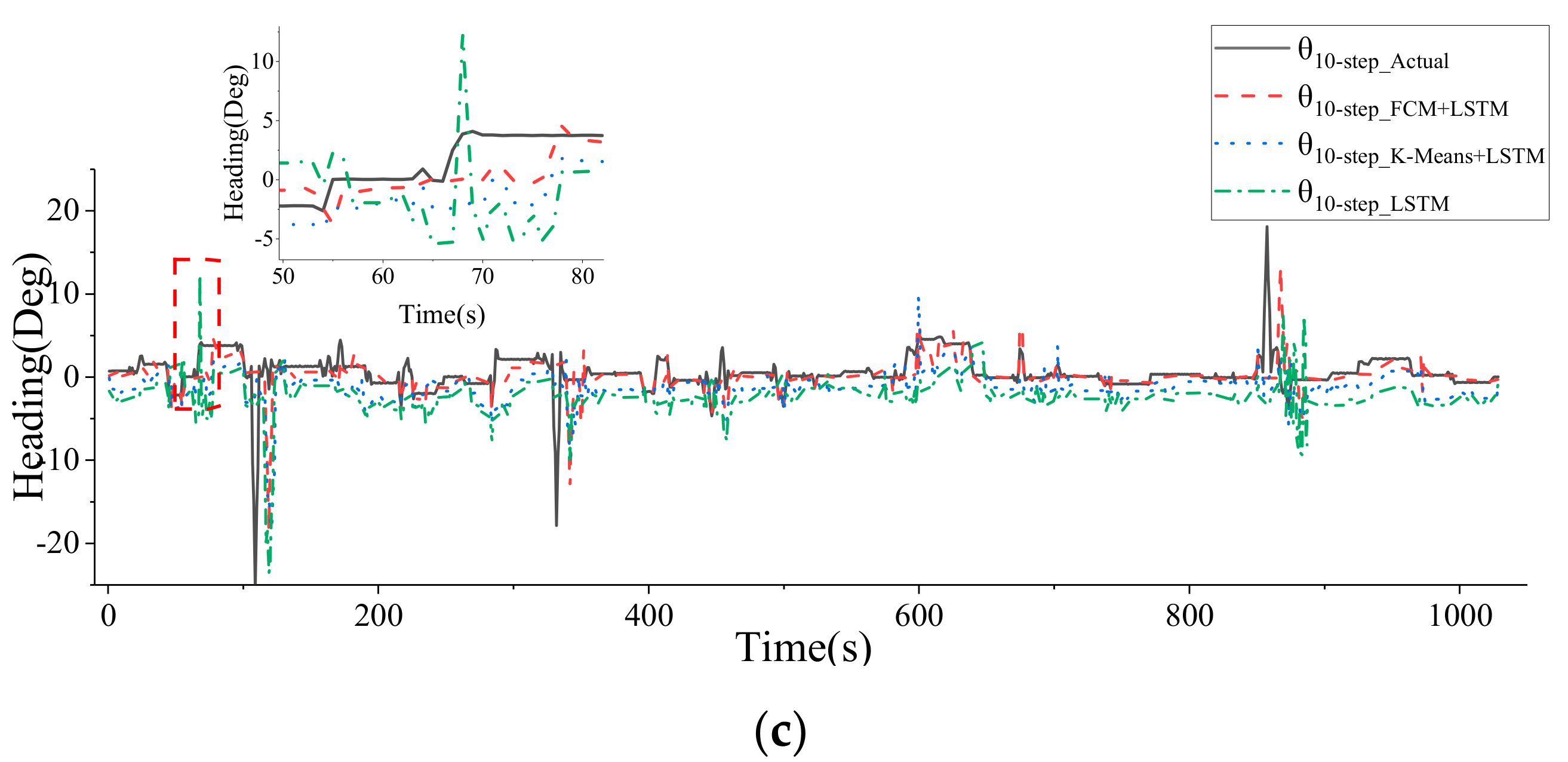
The results of multistep prediction for heading angle are shown in Figure 4 for the leading car, respectively, and the graphs show the prediction curves of heading angle for the third step length, the fifth step length, and the tenth step length. As seen from the graph, first of all, with the increase in the prediction step, each algorithm’s prediction results will appear with corresponding lag. The more prediction steps there are, the more significant the lag. Secondly, the prediction results of the other two methods are more aggressive than those of the algorithm adopted in this paper, which leads to an increase in the prediction error, especially in the course change operation; where the course angle changes more in a short period, the difference of the prediction results of the three methods is more obvious. The linear stability model based on FCM is more similar to the actual angle of attack of the vehicle in front of it, and the prediction error is reduced.
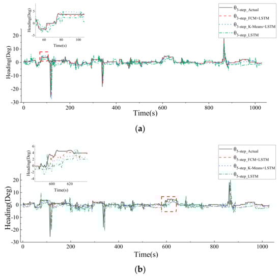
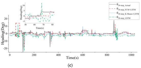
Figure 4.
Comparison of multistep heading angle prediction results: (a) comparison of the results of 3-step heading angle prediction; (b) comparison of the results of 5-step heading angle prediction; (c) comparison of the results of 10-step heading angle prediction.
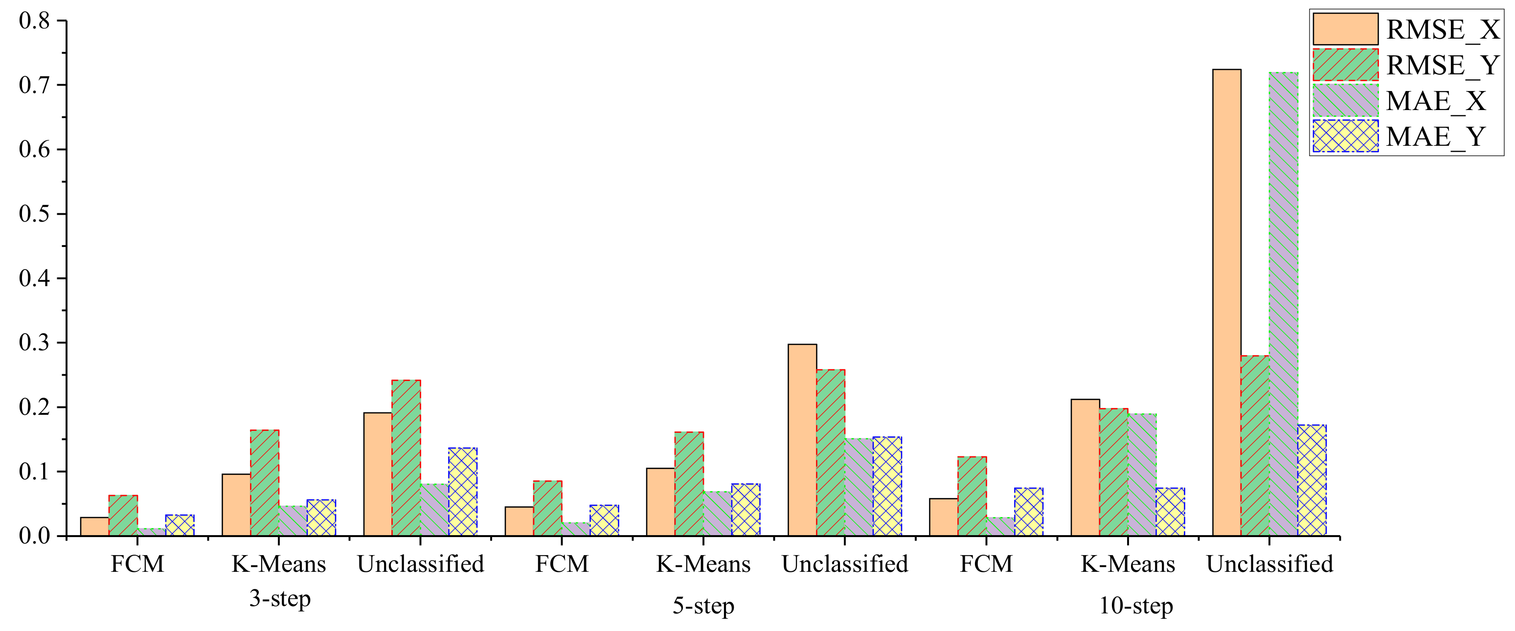
As shown in Figure 5, the comparison of RMSE and MAE of prediction in horizontal and vertical coordinates in the third step, fifth step, and tenth step using different prediction methods. Firstly, the three methods’ RMSE and MAE increased with the prediction step’s increase, especially in the tenth step. The RMSE and MAE values of the prediction algorithm without driving intent classification increased significantly in the horizontal coordinate compared to the fifth step, which proved that the prediction algorithm without driving intent classification was less effective at longer steps. Second, the RMSE and MAE values of the algorithm in this paper, both lower than the other two algorithms, prove the effectiveness of this algorithm.
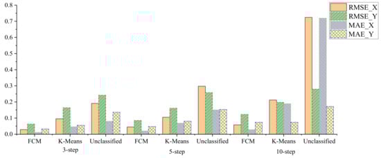
Figure 5.
Comparison figure of multistep prediction error.
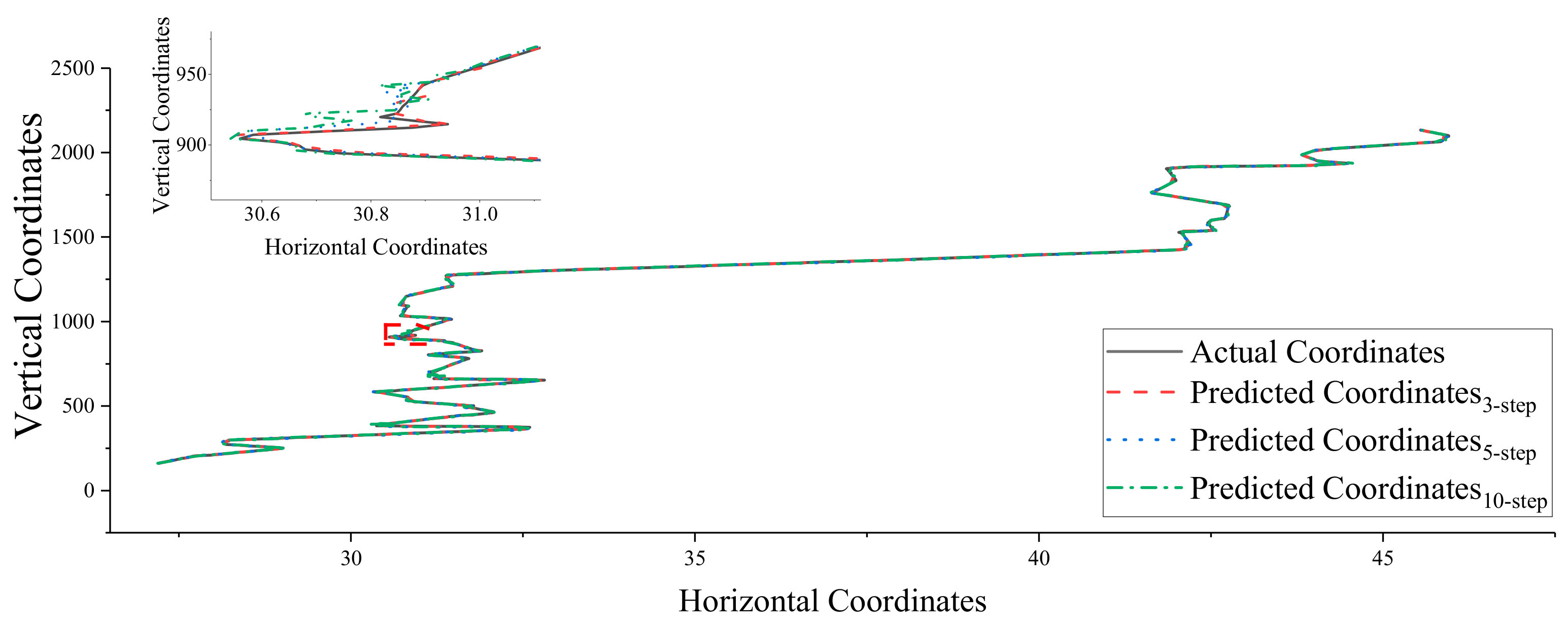
The trajectory prediction results of this algorithm are compared with the actual trajectory as shown in Figure 6. A 95% prediction error is less than 0.013 m for the tenth step horizontal distance. Of all the projected results, the maximum distance forecast error is 0.56 m. Of the vertical distance predictions, 95% had a prediction error of fewer than 0.025 m, and the maximum distance prediction error is 0.63 m.
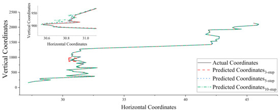
Figure 6.
Figure of multistep trajectory prediction results.
4. Conclusions
In this paper, we aimed to improve the prediction accuracy, reduce the influence of uncertainty of driving intention and dynamics of the leading vehicle on the prediction results, and construct a prediction algorithm based on driving intention classification. In order to accurately predict the future actions of the leading vehicle, instead of just predicting the coordinate points, this paper used the LSTM algorithm to predict the heading angle of the leading vehicle and the GPR algorithm to predict the speed. It combined them to calculate the future trajectory.
First, the impact on the future trajectory of the vehicle ahead under different driving intentions was fully considered, and the FCM algorithm was used to train the driving intentions of the vehicle ahead offline by taking the previous trajectory information and acceleration as input and using the information related to the speed and trajectory of the vehicle ahead under various complex working conditions. The output of FCM was the probability that the current input belongs to each category, and the final classification result was a probability set by the training dataset and the output classification probabilities to improve the resolution and accuracy of classification.
Second, the GPR model and the LSTM model were trained with the historical and current moment speed data and trajectory data of different driving intentions, and after the training was completed, the models output the speed and heading angle prediction results under different driving intentions.
Third, the FCM output affiliation function was used as the weight of each model to realize the variable gain weighted fusion of different driving intention prediction results and the joint calculation of heading angle and speed. An iterative rolling method predicts the target’s trajectory in the next 1s.
Finally, the algorithm was verified using real vehicle data, and the results showed that none of the horizontal prediction errors of the future 1s trajectory prediction results were greater than 0.013 m. All prediction results’ maximum values of horizontal distance prediction error reached 0.56 m. The vertical prediction error was no more than 0.025 m, and the maximum prediction error of the vertical distance among all the prediction results reached 0.63 m.
Author Contributions
Conceptualization, W.M. and Z.W.; software, W.M.; validation, W.M.; resources, W.M. and Z.W.; data curation, W.M.; writing—original draft preparation, W.M.; writing—review and editing, W.M. and Z.W.; visualization, W.M.; supervision, Z.W. All authors have read and agreed to the published version of the manuscript.
Funding
This research received no external funding.
Conflicts of Interest
The authors declare no conflict of interest.
References
- Lefèvre, S.; Sun, C.; Bajcsy, R.; Laugier, C. Comparison of parametric and non-parametric approaches for vehicle speed prediction. In Proceedings of the American Control Conference, Portland, OR, USA, 4–6 June 2014; IEEE: Piscataway, NJ, USA, 2014. [Google Scholar]
- Dai, S.; Li, L.; Li, Z. Modeling Vehicle Interactions via Modified LSTM Models for Trajectory Prediction. IEEE Access 2019, 7, 38287–38296. [Google Scholar] [CrossRef]
- Lin, L.; Li, W.; Bi, H.; Qin, L. Vehicle Trajectory Prediction Using LSTMs with Spatial–Temporal Attention Mechanisms. IEEE Intell. Transp. Syst. Mag. 2022, 14, 197–208. [Google Scholar] [CrossRef]
- Xie, G.; Gao, H.; Qian, L.; Huang, B.; Li, K.; Wang, J. Vehicle Trajectory Prediction by Integrating Physics- and Maneuver-Based Approaches Using Interactive Multiple Models. IEEE Trans. Ind. Electron. 2017, 65, 5999–6008. [Google Scholar] [CrossRef]
- Deo, N.; Rangesh, A.; Trivedi, M.M. How Would Surround Vehicles Move? A Unified Framework for Maneuver Classification and Motion Prediction. IEEE Trans. Intell. Veh. 2018, 3, 129–140. [Google Scholar] [CrossRef] [Green Version]
- Xiao, W.; Zhang, L.; Meng, D. Vehicle Trajectory Prediction Based on Motion Model and Maneuver Model Fusion with Interactive Multiple Models. SAE Int. J. Adv. Curr. Prac. Mobil. 2020, 2, 3060–3071. [Google Scholar]
- Ballan, L.; Castaldo, F.; Alahi, A.; Palmieri, F.; Savarese, S. Knowledge Transfer for Scene-Specific Motion Prediction; Springer: Cham, Switzerland, 2016. [Google Scholar]
- Ye, N.; Zhang, Y.; Wang, R. Vehicle trajectory prediction based on Hidden Markov Model. KSII Trans. Internet Inf. Syst. (TIIS) 2016, 10, 3150–3170. [Google Scholar]
- Choi, S.; Kim, J.; Yeo, H. Attention-based Recurrent Neural Network for Urban Vehicle Trajectory Prediction. Procedia Comput. Sci. 2019, 151, 327–334. [Google Scholar] [CrossRef]
- Ondruska, P.; Posner, I. Deep Tracking: Seeing Beyond Seeing Using Recurrent Neural Networks. In Proceedings of the Thirtieth AAAI Conference on Artificial Intelligence, Phoenix, AZ, USA, 12–17 February 2016. [Google Scholar]
- Kim, B.; Kang, C.M.; Kim, J.; Lee, S.H.; Chung, C.C.; Choi, J.W. Probabilistic Vehicle Trajectory Prediction over Occupancy Grid Map via Recurrent Neural Network. In Proceedings of the 2017 IEEE 20th International Conference on Intelligent Transportation Systems (ITSC), Yokohama, Japan, 16–19 October 2017; IEEE: Piscataway, NJ, USA, 2017. [Google Scholar]
- Choi, D.; Yim, J.; Baek, M.; Lee, S. Machine learning-based vehicle trajectory prediction using v2v communications and on-board sensors. Electronics 2021, 10, 420. [Google Scholar] [CrossRef]
- Shen, C.H.; Hsu, T.J. Research on Vehicle Trajectory Prediction and Warning Based on Mixed Neural Networks. Appl. Sci. 2020, 11, 7. [Google Scholar] [CrossRef]
- Liu, P.; Kurt, A.; Özgüner, Ü. Trajectory prediction of a lane changing vehicle based on driver behavior estimation and classification. In Proceedings of the 2014 17th IEEE International Conference on Intelligent Transportation Systems (ITSC), Qingdao, China, 8–11 October 2014; IEEE: Piscataway, NJ, USA, 2014. [Google Scholar]
- Gindele, T.; Brechtel, S.; Dillmann, R. A probabilistic model for estimating driver behaviors and vehicle trajectories in traffic environments. In Proceedings of the 13th International IEEE Conference on Intelligent Transportation Systems, Funchal, Portugal, 19–22 September 2010; IEEE: Piscataway, NJ, USA, 2010. [Google Scholar]
- Rákos, O.; Aradi, S.; Bécsi, T.; Szalay, Z. Compression of vehicle trajectories with a variational autoencoder. Appl. Sci. 2020, 10, 6739. [Google Scholar] [CrossRef]
- Woo, H.; Madokoro, H.; Sato, K.; Tamura, Y.; Yamashita, A.; Asama, H. Advanced adaptive cruise control based on operation characteristic estimation and trajectory prediction. Appl. Sci. 2019, 9, 4875. [Google Scholar] [CrossRef] [Green Version]
- Yuan, W.; Li, Z.; Wang, C. Lane-change prediction method for adaptive cruise control system with hidden Markov model. Adv. Mech. Eng. 2018, 10. [Google Scholar] [CrossRef] [Green Version]
- Han, T.; Jing, J.; Özgüner, Ü. Driving Intention Recognition and Lane Change Prediction on the Highway. In Proceedings of the 2019 IEEE Intelligent Vehicles Symposium (IV), Paris, France, 9–12 June 2019; pp. 957–962. [Google Scholar] [CrossRef] [Green Version]
- Kumar, P.; Perrollaz, M.; Lefevre, S.; Laugier, C. Learning-based approach for online lane change intention prediction. In Proceedings of the IEEE Intelligent Vehicles Symposium, Gold Coast, QLD, Australia, 23–26 June 2013; IEEE: Piscataway, NJ, USA, 2013. [Google Scholar]
- Liu, L.; Xu, G.Q.; Song, Z. Driver lane changing behavior analysis based on parallel Bayesian networks. In Proceedings of the Sixth International Conference on Natural Computation, Yantai, China, 10–12 August 2010; IEEE: Piscataway, NJ, USA, 2010. [Google Scholar]
- Wang, W.; Xi, J. A Rapid Pattern-Recognition Method for Driving Types Using Clustering-Based Support Vector Machines. In Proceedings of the 2016 American Control Conference (ACC), Boston, MA, USA, 6–8 July 2016; IEEE: Piscataway, NJ, USA, 2016; pp. 5270–5275. [Google Scholar]
- Jing, J.; Kurt, A.; Ozatay, E.; Michelini, J.; Filev, D.; Ozguner, U. Vehicle Speed Prediction in a Convoy Using V2V Communication. In Proceedings of the IEEE International Conference on Intelligent Transportation Systems, Gran Canaria, Spain, 15–18 September 2015; IEEE: Piscataway, NJ, USA, 2015. [Google Scholar]
- Wang, X.; Wang, H. Driving Behavior Clustering for Hazardous Material Transportation Based on Genetic Fuzzy C-Means Algorithm. IEEE Access 2020, 8, 11289–11296. [Google Scholar] [CrossRef]
- Liu, Y.; Wang, J.; Zhao, P.; Qin, D.; Chen, Z. Research on Classification and Recognition of Driving Styles Based on Feature Engineering. IEEE Access 2019, 7, 89245–89255. [Google Scholar] [CrossRef]
- Olsen, E. Modeling Slow Lead Vehicle Lane Changing. Ph.D. Thesis, Virginia Polytechnic Institute and State University, Blacksburg, VA, USA, 2003. [Google Scholar]
- Sun, C.; Sun, F.; He, H. Investigating adaptive-ECMS with velocity forecast ability for hybrid electric vehicles. Appl. Energy 2016, 185 Pt 2, 1644–1653. [Google Scholar] [CrossRef]
- Park, J.; Li, D.; Murphey, Y.L.; Kristinsson, J.; McGee, R.; Kuang, M.; Phillips, T. Real time vehicle speed prediction using a Neural Network Traffic Model. In Proceedings of the 2011 International Joint Conference on Neural Networks, San Jose, CA, USA, 31 July–5 August 2011; IEEE: Piscataway, NJ, USA, 2011. [Google Scholar]
- Zhao, J.; Sun, S. High-Order Gaussian Process Dynamical Models for Traffic Flow Prediction. IEEE Trans. Intell. Transp. Syst. 2016, 17, 2014–2019. [Google Scholar] [CrossRef]
- Moser, D.; Schmied, R.; Waschl, H.; del Re, L. Flexible Spacing Adaptive Cruise Control Using Stochastic Model Predictive Control. IEEE Trans. Control. Syst. Technol. 2017, 26, 114–127. [Google Scholar] [CrossRef]
- Zhang, B.; Zhang, J.; Xu, F.; Shen, T. Optimal control of power-split hybrid electric powertrains with minimization of energy consumption. Appl. Energy 2020, 266, 114873. [Google Scholar] [CrossRef]
- Xu, F.; Shen, T. Look-Ahead Prediction-Based Real-Time Optimal Energy Management for Connected HEVs. IEEE Trans. Veh. Technol. 2020, 69, 2537–2551. [Google Scholar] [CrossRef]
- Hochreiter, S.; Schmidhuber, J. Long Short-Term Memory. Neural Comput. 1997, 9, 1735–1780. [Google Scholar] [CrossRef] [PubMed]
- Girard, A.; Rasmussen, C.E.; Candela, J.Q.; Murray-Smith, R. Gaussian Process Priors with Uncertain Inputs-Application to Mutiple-Step ahead Time Series Forecasting. In Advances in Neural Information Processing Systems; MIT Press: Cambridge, MA, USA, 2003; Volume 15, pp. 542–552. [Google Scholar]
- Hachino, T.; Kadirkamanathan, V. Time Series Forecasting Using Multiple Gaussian Process Prior Model. In Proceedings of the IEEE Symposium on Computational Intelligence & Data Mining, Honolulu, HI, USA, 1 March–5 April 2007. [Google Scholar]
- Yan, W.; Qiu, H.; Xue, Y. Gaussian process for long-term time-series forecasting. In Proceedings of the International Joint Conference on Neural Networks, Atlanta, GA, USA, 14–19 June 2009; IEEE: Piscataway, NJ, USA, 2009. [Google Scholar]
Publisher’s Note: MDPI stays neutral with regard to jurisdictional claims in published maps and institutional affiliations. |
© 2022 by the authors. Licensee MDPI, Basel, Switzerland. This article is an open access article distributed under the terms and conditions of the Creative Commons Attribution (CC BY) license (https://creativecommons.org/licenses/by/4.0/).