An MHD Marangoni Boundary Layer Flow and Heat Transfer with Mass Transpiration and Radiation: An Analytical Study

Abstract

This examination is carried out on the two-dimensional magnetohydrodynamic problem for a steady incompressible flow over a porous medium. The $Cu-A{l}_2{O}_3$ nanoparticles are added to the water base fluid in order to improve thermal efficiency. The transverse magnetic field with strength $B_0$ is applied. The governing equations formed for the defined flow form a system of partial differential equations that are then converted to a system of ordinary differential equations upon applying the suitable similarity transformations. On analytically solving the obtained system, the solutions for velocity profile and temperature distribution are obtained in terms of exponential and Gamma functions, respectively. In addition, the physical parameter of interest, the local Nusselt number, is obtained. The results are analyzed through plotting graphs, and the effect of different parameters is analyzed. Furthermore, we observe that the suction/injection parameter enhances the axial velocity. The porous and radiation parameters enhance the temperature distribution, and the suction/injection parameter suppresses the temperature distribution.

1. Introduction

Several studies have focused on the problem of boundary layer flow (BLF) and heat transfer across a stretching/shrinking sheet [1]. Because of its importance in industrial and engineering processes, a significant amount of effort has been devoted to this area in recent years. The application of certain flows in engineering and technological operations includes refrigeration, electrical gadgets with fans, nuclear reactors, polyethylene extraction, steel fabrication, and many more. Crane introduced the idea of flow across a stretching sheet by analytically solving the steady 2D flow through a linearly stretched plat [1]. Wang further generalized this concept to a 3D example [2]. Numerous scholars have since investigated various facets of this form of movement [3,4,5,6,7,8,9,10]. They examined fluid flow and even heat transfer properties of a permeable stretching sheet of convective boundary conditions (BCs), viscous dissipation, and several types of fluid.

Choi was the first to invent the phrase “nanofluid” (NF) in 1995 [11], which is a mixture that improves the physical and chemical properties of a fluid using nanoparticles. Currently, the importance of energy consumption has led scientists to optimize thermal devices. One of the solutions proposed for this purpose is using solid nanoparticles to amend the thermal properties of conventional viscous fluids. Furthermore, a different type of NF, called a hybrid nanofluid (HNF), is being studied to boost the mass transfer coefficient even more. HNF is an enhanced NF composed of two unique nanoparticles, while ordinary NF consists of a special nanoparticle that absorbs the base fluid. The chemical compositions of HNF are then improved, which improves mass transfer efficiency. Most of the studies investigated the BLF and mass transfer. The concept of HNF has been the subject of extensive scientific studies. It was proven that hybrid nanofluids can be an alternative to the single nanofluid, because it can provide more heat transfer enhancement, particularly in the contexts of solar energy, electromechanics and automobile use.

Mahabaleshwar et al. studied the radiation effect on inclined MHD flow and found the exact solution for the flow over the porous media by considering different boundary conditions, such as on the studied MHD flow with CNTs by considering the impact of mass transpiration and radiation, on the flow and heat transfer with chemical reaction in porous media, as well as on the unsteady inclined MHD flow for Casson HNF due to porous media [12,13]. Moreover, Aly and Pop [14] performed a comparison between the significance of HNF and NF on MHD flow and heat transfer by considering the effect of partial slip. The flow of MHD in such a particular case was first explored by Sarpakaya [15] and Mahabaleshwar [16]. Mahabaleshwar et al. [17] investigated the MHD effect on a Newtonian fluid flow due to a super-linear stretching sheet. Fang and Zhang [18] and Hamad [19] examined the MHD flow due to a shrinking sheet and a stretching sheet, respectively. Turkyilmazoglu [20] examined the MHD flow, heat and mass transfer of viscoelastic fluid with slip over the stretching surface, and obtained multiple solutions. Suresh et al. [21,22] investigated the effect of HNF on heat transfer and the formation of HNF out of (Al₂O₃-Cu/H₂O). Vinay Kumar et al. [23] also investigated the MHD flow over a nonlinear stretching/shrinking sheet and the impact of slip on it in a porous medium.

On the other hand, many studies have been conducted on HNF flow, MHD HNF flow due to a quadratic stretching/shrinking sheet, radiative mixed convective flow, and also dusty HNF [24,25]. Furthermore, recent developments and applications of HNF were investigated in Refs. [26,27].

The Marangoni convection is stress due to the transverse gradient of surface tension that is acting along interfaces to produce movements in liquid–liquid or liquid–gas interfaces in some industrial processes. The thermo-Marangoni convection has important applications in the semiconductor and metallurgical industries, as well as in welding and crystal growth [27,28,29]. Chamkha [30] demonstrated that surface-driven flows, which may be produced not only by Marangoni effects but also by the existence of the buoyancy effects caused by gravity and the external pressure gradient, can produce steady boundary layers along the interface of two immiscible fluids. Motivated by the aforementioned works, the aim of the current study was to examine the 2D MHD steady incompressible flow and heat transfer of HNF over a porous medium. In particular, we included the effect of adding $Cu-A{l}_2{O}_3$ nanoparticles to the base fluid water in order to improve thermal efficiency. The thermal conductivity of $Cu-A{l}_2{O}_3$ water increases with increasing volume concentration of nanoparticles. The main reason for the increase in thermal conductivity of $Cu-A{l}_2{O}_3$ water hybrid nanofluid is the functionalization of $A{l}_2{O}_3$ and $Cu$ nanoparticles, which have a higher thermal conductivity than $A{l}_2{O}_3$ nanoparticles. Thermal radiation was also incorporated in the present study. Because of its impact on processes that operate at high temperatures, thermal radiation has also drawn a lot of interest [31,32,33]. We performed an analysis to obtain the velocity profile and temperature distribution for this system. The manuscript is arranged as follows: In Section 2, the physical model is presented and, in Section 3, the analytical solutions of the model are obtained. In Section 4, the results are discussed. Finally, the concluding remarks are given in Section 5.

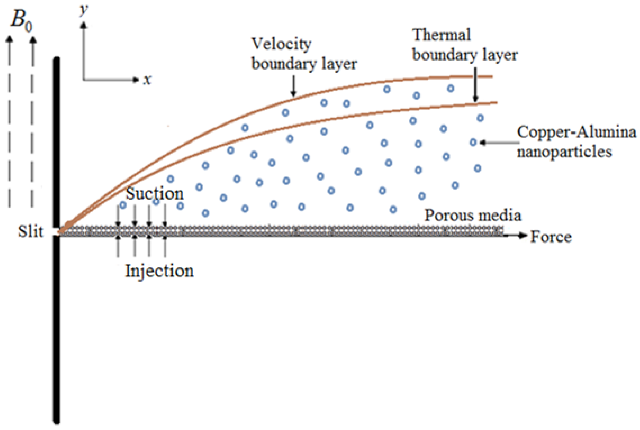
2. Physical Model

The 2D MHD steady incompressible flow and heat transfer of HNF over a porous medium are here considered. As shown in Figure 1, the transverse magnetic field with strength $B_0$ is applied along the y-axis. In addition, the $Cu$ and $A{l}_2{O}_3$ nanoparticles are added to the water base fluid. This shows that the velocity boundary layer thickness is more than the thermal boundary layer thickness. The ambient temperature of the HNF is kept constant at $T_{\infty }$. In adopting the standard boundary layer approximation, the leading equations are as follows [27],

$$\frac{\partial u}{\partial x}+\frac{\partial \mathrm{v}}{\partial y}=0$$

(1)

$$u\frac{\partial u}{\partial x}+\mathrm{v}\frac{\partial u}{\partial y}=\frac{{\mu }_{eff}}{{\rho }_{hnf}}\frac{{\partial }^{2}u}{\partial y^2}-\frac{{\sigma }_{hnf}{B}_0^2}{{\rho }_{hnf}}u-\frac{{\mu }_{hnf}}{{\rho }_{hnf}K}u$$

(2)

$$u\frac{\partial T}{\partial x}+\mathrm{v}\frac{\partial T}{\partial y}=\frac{{\kappa }_{hnf}}{{\left(\rho C_P\right)}_{hnf}}\frac{{\partial }^{2}T}{\partial y^2}-\frac{1}{{\left(\rho C_P\right)}_{hnf}}\frac{\partial q_r}{\partial y}$$

(3)

subject to BCs,

$$\begin{array}{l}\mathrm{v}={\mathrm{v}}_w\hspace{0.17em}\hspace{0.17em},\hspace{0.17em}\hspace{0.17em}{\mu }_{hnf}\frac{\partial u}{\partial y}=\frac{\partial \sigma }{\partial T}\frac{\partial T}{\partial x}\hspace{0.17em}\hspace{0.17em}\hspace{0.17em}\hspace{0.17em}\mathrm{at}\hspace{0.17em}\hspace{0.17em}\hspace{0.17em}y=0,\\ u\to 0\hspace{0.17em}\hspace{0.17em}\hspace{0.17em}\hspace{0.17em}\hspace{0.17em}\hspace{0.17em},\hspace{0.17em}\hspace{0.17em}T\to T_{\infty }\hspace{0.17em}\hspace{0.17em}\hspace{0.17em}\hspace{0.17em}\hspace{0.17em}\hspace{0.17em}\hspace{0.17em}\hspace{0.17em}\hspace{0.17em}\hspace{0.17em}\mathrm{as}\hspace{0.17em}\hspace{0.17em}\hspace{0.17em}y\to \infty \end{array}\}$$

(4)

All mentioned parameters are as described in the nomenclature. The subscript $hnf$ denotes the HNF quantities and are described as below,

$$\frac{{\rho }_{hnf}}{{\rho }_f}=\left(1-{\varphi }_2\right)\left(1-{\varphi }_1+{\varphi }_1\frac{{\rho }_{s_1}}{{\rho }_f}\right)+{\varphi }_2\left(\frac{{\rho }_{s_2}}{{\rho }_f}\right)$$

$$\begin{gathered} \frac{{\mu }_{hnf}}{{\mu }_f}=\frac{1}{{\left(1-{\varphi }_1\right)}^{2.5}{\left(1-{\varphi }_2\right)}^{2.5}}\hspace{0.17em}\hspace{0.17em}\hspace{0.17em}\hspace{0.17em}\hspace{0.17em}\hspace{0.17em}\hspace{0.17em}\hspace{0.17em}\hspace{0.17em} \\ \frac{{\sigma }_{hnf}}{{\sigma }_f}=\frac{{\sigma }_{s_2}+2{\sigma }_{bf}+2{\varphi }_2\left({\sigma }_{s_2}-{\sigma }_f\right)}{{\sigma }_{s_2}+2{\sigma }_{bf}-{\varphi }_2\left({\sigma }_{s_2}-{\sigma }_f\right)}, \end{gathered}$$

where

$$\begin{gathered} \frac{{\sigma }_{bf}}{{\sigma }_f}=\frac{{\sigma }_{s_1}+2{\sigma }_f+2{\varphi }_1\left({\sigma }_{s_1}-{\sigma }_f\right)}{{\sigma }_{s_1}+2{\sigma }_f-{\varphi }_1\left({\sigma }_{s_1}-{\sigma }_f\right)}\hspace{0.17em} \\ \frac{k_{hnf}}{k_f}=\frac{k_{s_2}+2k_{bf}+2{\varphi }_2\left(k_{s_2}-k_f\right)}{k_{s_2}+2k_{bf}-{\varphi }_2\left(k_{s_2}-k_f\right)}, \end{gathered}$$

where

$$\frac{k_{bf}}{k_f}=\frac{k_{s_1}+2k_f+2{\varphi }_1\left(k_{s_1}-k_f\right)}{k_{s_1}+2k_f-{\varphi }_1\left(k_{s_1}-k_f\right)}$$

$$\frac{{\left(\rho C_P\right)}_{hnf}}{{\left(\rho C_P\right)}_f}=\left(1-{\varphi }_2\right)\left(1-{\varphi }_1+{\varphi }_1\frac{{\left(\rho C_p\right)}_{s_1}}{{\left(\rho C_p\right)}_f}\right)+{\varphi }_2\frac{{\left(\rho C_p\right)}_{s_2}}{{\left(\rho C_P\right)}_f}$$

(5)

The radiative heat flux is calculated by applying the Rosseland approximation for radiation as follows [12,28],

$$q_r=-\frac{4{\sigma }^{*}}{3k^{*}}\frac{\partial T^4}{\partial y}$$

(6)

It is implicit that the temperature varies within the flow, where the term $T^4$ is the linear function of the temperature. Therefore, using Taylor series expansion to the term $T^4$ about $T_{\infty }$ and ignoring the higher order terms, we acquire

$$T^4\cong 4T_{\infty }^{3}T-3T_{\infty }^4$$

(7)

Equation (3) reduces to

$$u\frac{\partial T}{\partial x}+\mathrm{v}\frac{\partial T}{\partial y}=\frac{{\kappa }_{hnf}}{{\left(\rho C_P\right)}_{hnf}}\frac{{\partial }^{2}T}{\partial y^2}+\frac{16{\sigma }^{*}{T}_{\infty }^3}{3k^{*}{\left(\rho C_P\right)}_{hnf}}\frac{{\partial }^{2}T}{\partial y^2}$$

(8)

Consider the suitable similarity transformations as follows [27]:

$$\begin{array}{l}\psi \left(\eta \right)={\xi }_{2}xf\left(\eta \right),\eta ={\xi }_{1}y\hspace{0.17em}\\ u={\xi }_1{\xi }_{2}x{f}_{\eta }\left(\eta \right),\hspace{0.17em}\mathrm{v}=-{\xi }_{2}f\left(\eta \right)\hspace{0.17em},\hspace{0.17em}\theta \left(\eta \right)=\frac{T-T_{\infty }}{a{x}^2}\hspace{0.17em}\hspace{0.17em}\hspace{0.17em}\end{array}$$

(9)

On using (9), Equations (2) to (4) are converted as

$$\mathsf{\Lambda }{f}_{\eta \eta \eta }+C_1\left(f{f}_{\eta \eta }-f_{\eta }{}^2\right)-\left(C_{3}M+C_{2}D{a}^{-1}\right)f_{\eta }=0$$

(10)

$$\frac{1}{C_4}\left(\frac{C_5}{\mathrm{Pr}}+N_R\right){\theta }_{\eta \eta }+f{\theta }_{\eta }-2f_{\eta }\theta =0$$

(11)

With the imposed BCs as

$$\begin{array}{l}f\left(0\right)=S\hspace{0.17em}\hspace{0.17em},\hspace{0.17em}\hspace{0.17em}{f}_{\eta \eta }\left(0\right)=-2{\left(1-{\varphi }_1\right)}^{2.5}{\left(1-{\varphi }_2\right)}^{2.5}\hspace{0.17em}\hspace{0.17em},\hspace{0.17em}\hspace{0.17em}\theta \left(0\right)=1,\\ f_{\eta }\left(\eta \right)\to 0\hspace{0.17em}\hspace{0.17em},\hspace{0.17em}\hspace{0.17em}\theta \left(\eta \right)\to 0\hspace{0.17em}\hspace{0.17em}\hspace{0.17em}as\hspace{0.17em}\hspace{0.17em}\hspace{0.17em}\eta \to \infty \end{array}\}$$

(12)

where $D{a}^{-1}=\frac{{\nu }_f}{K{\xi }_1{\xi }_2}$ is the inverse Darcy number; $\mathsf{\Lambda }=\frac{{\mu }_{eff}}{{\mu }_f}$ is the Brinkman ratio; $M=\frac{{\sigma }_f{B}_0{}^2}{{\xi }_1{\xi }_2{\nu }_f}$ is the magnetic field; $N_R=\frac{16{\sigma }^{*}{T}_{\infty }{}^3}{3k_f{k}^{*}}$ is thermal radiation; and $C_i$, where i = 1 to 5, is taken as

$$C_1=\frac{{\rho }_{hnf}}{{\rho }_f}\hspace{0.17em}\hspace{0.17em},\hspace{0.17em}\hspace{0.17em}{C}_2=\frac{{\mu }_{hnf}}{{\mu }_f}\hspace{0.17em}\hspace{0.17em},\hspace{0.17em}\hspace{0.17em}{C}_3=\frac{{\sigma }_{hnf}}{{\sigma }_f}\hspace{0.17em}\hspace{0.17em},\hspace{0.17em}\hspace{0.17em}{C}_4=\frac{{\left(\rho C_P\right)}_{hnf}}{{\left(\rho C_P\right)}_f}\hspace{0.17em}\hspace{0.17em}\hspace{0.17em}\mathrm{and}\hspace{0.17em}\hspace{0.17em}\hspace{0.17em}{C}_5=\frac{k_{hnf}}{k_f}$$

(13)

The interested physical local Nusselt number $N{u}_x$ is given by

$$N{u}_x=\frac{x{q}_w}{k_f\left(T-T_{\infty }\right)}$$

(14)

where $q_w$ is the heat flux given as

$$q_w=-k_{hnf}{\left(\frac{\partial T}{\partial y}+q_r\right)}_{y=0}$$

(15)

Equations (14) and (15) lead to

$$N{u}_x=-\left(\frac{k_{hnf}}{k_f}-k_{hnf}\mathrm{Pr}{N}_R\right){\xi }_{1}x{\theta }_{\eta }\left(0\right)$$

(16)

3. Exact Analytical Solutions

In this section, we compute the analytical solution of the model. We separate the section into two subsections for the velocity and temperature fields.

3.1. Velocity

The exact analytical solution of Equation (10) is in the form

$$f\left(\eta \right)=d_1+d_2{e}^{-\alpha \eta }$$

(17)

where $\alpha >0$ is to be determined. On using BCs (12a)

$$\begin{gathered} d_1=S-d_2\hspace{0.17em}\hspace{0.17em}\hspace{0.17em}\hspace{0.17em}\hspace{0.17em}\hspace{0.17em}\hspace{0.17em}\hspace{0.17em}\hspace{0.17em}\hspace{0.17em}\hspace{0.17em}\hspace{0.17em}\hspace{0.17em}\hspace{0.17em} \\ \hspace{0.17em}\hspace{0.17em}\hspace{0.17em}\hspace{0.17em}\hspace{0.17em}\hspace{0.17em}\hspace{0.17em}\hspace{0.17em}\hspace{0.17em}\hspace{0.17em}\hspace{0.17em}\hspace{0.17em}{d}_2=-\frac{2}{{\alpha }^2}{\left(1-{\varphi }_1\right)}^{2.5}{\left(1-{\varphi }_2\right)}^{2.5} \end{gathered}$$

(18)

So, using (17) in Equation (10) gives

$$\mathsf{\Lambda }{\alpha }^3-S{C}_1{\alpha }^2-\left(C_{3}M+C_{2}D{a}^{-1}\right)\alpha -2C_1{\left(1-{\varphi }_1\right)}^{2.5}{\left(1-{\varphi }_2\right)}^{2.5}=0$$

(19)

3.2. Temperature Distribution $\theta \left(\eta \right)$

Using Equation (17) and applying a new variable $\epsilon =-e^{-\alpha \eta }$ in Equation (11),

$$\epsilon {\theta }_{\epsilon \epsilon }\left(\epsilon \right)+\left(p-q\epsilon \right){\theta }_{\epsilon }\left(\epsilon \right)+2q\theta \left(\epsilon \right)=0$$

(20)

with BCs as

$$\theta \left(0\right)=0\hspace{0.17em}\hspace{0.17em},\hspace{0.17em}\hspace{0.17em}\theta \left(-1\right)=1,$$

(21)

where $p=1-\frac{n}{\alpha }\left[S+\frac{2}{{\alpha }^2}{\left(1-{\varphi }_1\right)}^{2.5}{\left(1-{\varphi }_2\right)}^{2.5}\right]$ and $q=\frac{2n}{{\alpha }^3}{\left(1-{\varphi }_1\right)}^{2.5}{\left(1-{\varphi }_2\right)}^{2.5}$, where $n=\frac{C_4}{\left(\frac{C_5}{\mathrm{Pr}}+N_R\right)}$.

To solve Equation (20), we deploy the Laplace transformation to obtain

$$S\left(q-S\right){\mathsf{\Theta }}_S\left(S\right)+\left[3q+S\left(p-2\right)\right]\mathsf{\Theta }\left(S\right)=0$$

(22)

Here, $\mathsf{\Theta }\left(S\right)=L\left[\theta \left(\epsilon \right)\right]$. Integrating Equation (22) gives

$$\mathsf{\Theta }\left(S\right)=\frac{C{\left(S-q\right)}^{\left(p+1\right)}}{S^3}$$

(23)

In order to obtain the solution of Equation (20), we apply the inverse Laplace transformation and use the convolution property to acquire

$$\theta \left(t\right)=\frac{C}{2\mathsf{\Gamma }\left[-1-p\right]}{\displaystyle \underset{0}{\overset{t}{\int }}\frac{{\left(t-w\right)}^2}{w^{p+2}}exp\left(qw\right)dw}, \mathrm{here} p<-1$$

(24)

where $C$ is integrating constant can be determined by using the BCs $\theta \left(-1\right)=1$ in Equation (24) to obtain,

$$C=\frac{2\mathsf{\Gamma }\left[-1-p\right]}{{\displaystyle \underset{0}{\overset{-1}{\int }}\frac{{\left(1+w\right)}^2}{w^{p+2}}exp\left(qw\right)dw}}$$

(25)

Therefore, Equation (24) becomes

$$\theta \left(\epsilon \right)=-\frac{{\displaystyle \underset{0}{\overset{\epsilon }{\int }}\frac{{\left(\epsilon -w\right)}^2}{w^{p+2}}exp\left(qw\right)dw}}{{\displaystyle \underset{-1}{\overset{0}{\int }}\frac{{\left(1+w\right)}^2}{w^{p+2}}exp\left(qw\right)dw}}$$

(26)

Operating the integration of Equation (26) gives the final expression for $\theta \left(t\right)$

$$\theta \left(\epsilon \right)=\frac{q^2{\epsilon }^2\mathsf{\Gamma }\left[-p-1,0,-q\epsilon \right]+2q\epsilon \hspace{0.17em}\mathsf{\Gamma }\left[-p,0,-q\epsilon \right]+\mathsf{\Gamma }\left[-p+1,0,-q\epsilon \right]}{q^2\mathsf{\Gamma }\left[-p-1,0,q\right]-2q\mathsf{\Gamma }\left[-p,0,q\right]+\mathsf{\Gamma }\left[-p+1,0,q\right]}$$

(27)

In terms of the similarity variable $\eta$, Equation (27) becomes:

$$\theta \left(\eta \right)=\frac{q^2{e}^{-2\alpha \eta }\hspace{0.17em}\mathsf{\Gamma }\left[-p-1,0,q{e}^{-\alpha \eta }\right]-2q{e}^{-\alpha \eta }\hspace{0.17em}\mathsf{\Gamma }\left[-p,0,q{e}^{-\alpha \eta }\right]+\mathsf{\Gamma }\left[-p+1,0,q{e}^{-\alpha \eta }\right]}{q^2\mathsf{\Gamma }\left[-p-1,0,q\right]-2q\mathsf{\Gamma }\left[-p,0,q\right]+\mathsf{\Gamma }\left[-p+1,0,q\right]}$$

(28)

Differentiating Equation (28), we obtain

$${\theta }_{\eta }\left(0\right)=\frac{2\alpha q\left\{\mathsf{\Gamma }\left[-p,0,q\right]-q\mathsf{\Gamma }\left[-p-1,0,q\right]\right\}}{q^2\mathsf{\Gamma }\left[-p-1,0,q\right]-2q\mathsf{\Gamma }\left[-p,0,q\right]+\mathsf{\Gamma }\left[-p+1,0,q\right]}$$

(29)

Therefore, from Equation (16,) Nusselt number becomes

$$N{u}_x=-\left(\frac{k_{hnf}}{k_f}-k_{hnf}\mathrm{Pr}{N}_R\right){\xi }_{1}x\frac{2\alpha q\left\{\mathsf{\Gamma }\left[-p,0,q\right]-q\mathsf{\Gamma }\left[-p-1,0,q\right]\right\}}{q^2\mathsf{\Gamma }\left[-p-1,0,q\right]-2q\mathsf{\Gamma }\left[-p,0,q\right]+\mathsf{\Gamma }\left[-p+1,0,q\right]}$$

(30)

In the next section, we analyze these results.

4. Results and Discussion

We examined the 2D MHD steady incompressible flow and heat transfer due to a porous medium containing $Cu-A{l}_2{O}_3$ nanoparticles in the base fluid by applying a magnetic field of strength $B_0$ to the fluid flow. The addition of nanoparticles enhances the thermal efficiency of the flow system. The leading equations form the system of PDEs and are then converted into the system of ODEs by adopting suitable similarity transformations. The system is analytically solved to obtain the solutions for the velocity profile and temperature distribution in terms of exponential and Gamma functions, respectively. In all plots, the dotted lines refer to the behavior of the base fluid, while the solid lines refer to the behavior of HNF for $Cu-A{l}_2{O}_3$.

Figure 2 demonstrates the axial velocity $f\left(\eta \right)$ for various $D{a}^{-1}$. We found that the velocity declines as $D{a}^{-1}$ increases. Panels (a)–(c), where the velocity is examined for $S=0$ show that there is no permeability. For suction $S=1$ and injection $S=-1$, we observe that as $S$ increases from injection to suction, the axial velocity for HNF very quickly coincides with the base fluid as $D{a}^{-1}$ increases. In all cases, the profile of $f_{\eta }\left(\eta \right)$ has a decreasing nature, and it becomes constant to zero at a certain point of $\eta$.

Figure 3 depicts the velocity $f_{\eta }\left(\eta \right)$ as a function of $\eta$ for various values of $\mathsf{\Lambda }$. The velocity increases with an increase in $\mathsf{\Lambda }$. Panels (a)–(c), where the velocity is examined for $S=0$, show that there is no permeability. For suction $S=1$ and injection $S=-1$, we observe that the difference between the axial velocity of the base fluid and HNF is larger in the case of suction and smaller in the case of injection. In all cases, the axial velocity is less for an HNF than the base fluid.

Figure 4 shows the profile of $f_{\eta }\left(\eta \right)$ for various $M$. It can be seen that $f_{\eta }\left(\eta \right)$ is smaller for larger values of $M$. Panels (a)–(c), where the velocity is examined for $S=0$, show that there is no permeability. For suction $S=1$ and injection $S=-1$, we observe that the difference between the axial velocity of the base fluid and the HNF is more in the case of suction and less in the case of injection.

The effect of S is shown in Figure 5 for both the suction and injection cases. Clearly, the velocity profile $f_{\eta }\left(\eta \right)$ decreases for a larger $S$. Panel (a) shows that the difference between the axial velocity of the base fluid and the HNF is larger in the case of suction and smaller in the case of injection as in panel (b). At $\eta =0$, the axial velocity is different for various values of each parameter.

Figure 6 displays the temperature profile $\theta \left(\eta \right)$ for various values of $D{a}^{-1}$. We observe that $\theta \left(\eta \right)$ increases as $D{a}^{-1}$ increases. Panels (a)–(c), where the temperature is shown for $S=0$, show that there is no permeability. For suction $S=1$ and injection $S=-1$, we observe that $\theta \left(\eta \right)$ for HNF coincides with the base fluid as $D{a}^{-1}$ increases. In all cases, we found that $\theta \left(\eta \right)$ decreases and that becomes constant to zero at a certain point of $\eta$. The temperature profile has the same value at $\eta =0$ irrespective of the parameters’ values. Moreover, as the thermal rate increases upon adding nanoparticles to the base fluid, we can see from the figures that $\theta \left(\eta \right)$ becomes more of an HNF than a base fluid.

Figure 7 shows the temperature profile $\theta \left(\eta \right)$ for different values $\mathsf{\Lambda }$. We observe that $\theta \left(\eta \right)$ decreases with the enhancement in $\mathsf{\Lambda }$. Panels (a)–(c) show the regimens of S. In panel (a) for $S=0$, there is no permeability, whereas in panel (b) suction $\left(S=1\right)$ and finally in panel (c) for injection case $\left(S=-1\right)$. We found that there is an achievement of enhancement of heat transfer upon using HNF and that Casson fluid will suppress the temperature distribution.

Figure 8 shows the temperature profile as a function of $\eta$ for different values of $M$. We see that $\theta \left(\eta \right)$ increases as $M$ increases. Panels (a)–(c) show $\theta$ for $S=0$, $S=1$, and $S=-1$, respectively. We observe that HNF has much more thermal conductivity than the base fluid. Furthermore, we observe that as the value of S increases, the domain of the temperature distribution decreases.

Figure 9 shows the temperature distribution $\theta \left(\eta \right)$ for various values of the radiation parameter $N_R$. We can observe that $\theta \left(\eta \right)$ increases as the effect of radiation increases. Panels (a)–(c) show the profile for cases with no permeability, with suction and injection. We note that the domain of the temperature is larger in the case of injection and smaller in the case of no-permeability. Furthermore, by observing each plot of temperature distribution, the effect of radiation on the change of heat transfer rate is less than those of the magnetic field and Casson fluid, i.e., the difference in temperature distribution between base fluid and HNF is not that much more significant.

Finally, the effect of various values of $S$ on the temperature profile is shown in Figure 10 for suction and injection cases. $\theta \left(\eta \right)$ decreases when as $S$ increases, as shown in the figure. The domain of $\theta \left(\eta \right)$ is larger in the case of injection than in suction.

5. Concluding Remarks

In the present study, we examined 2D MHD steady incompressible flow and heat transfer over a porous medium containing $Cu-A{l}_2{O}_3$ nanoparticles in a base fluid. The addition of nanoparticles enhances the thermal efficiency of the flow system. The system was analytically solved to obtain the solutions for the velocity profile and temperature distribution in terms of exponential and Gamma functions, respectively. In addition, the effect of different physical parameters was examined by using graphical representations. The following observations were made:

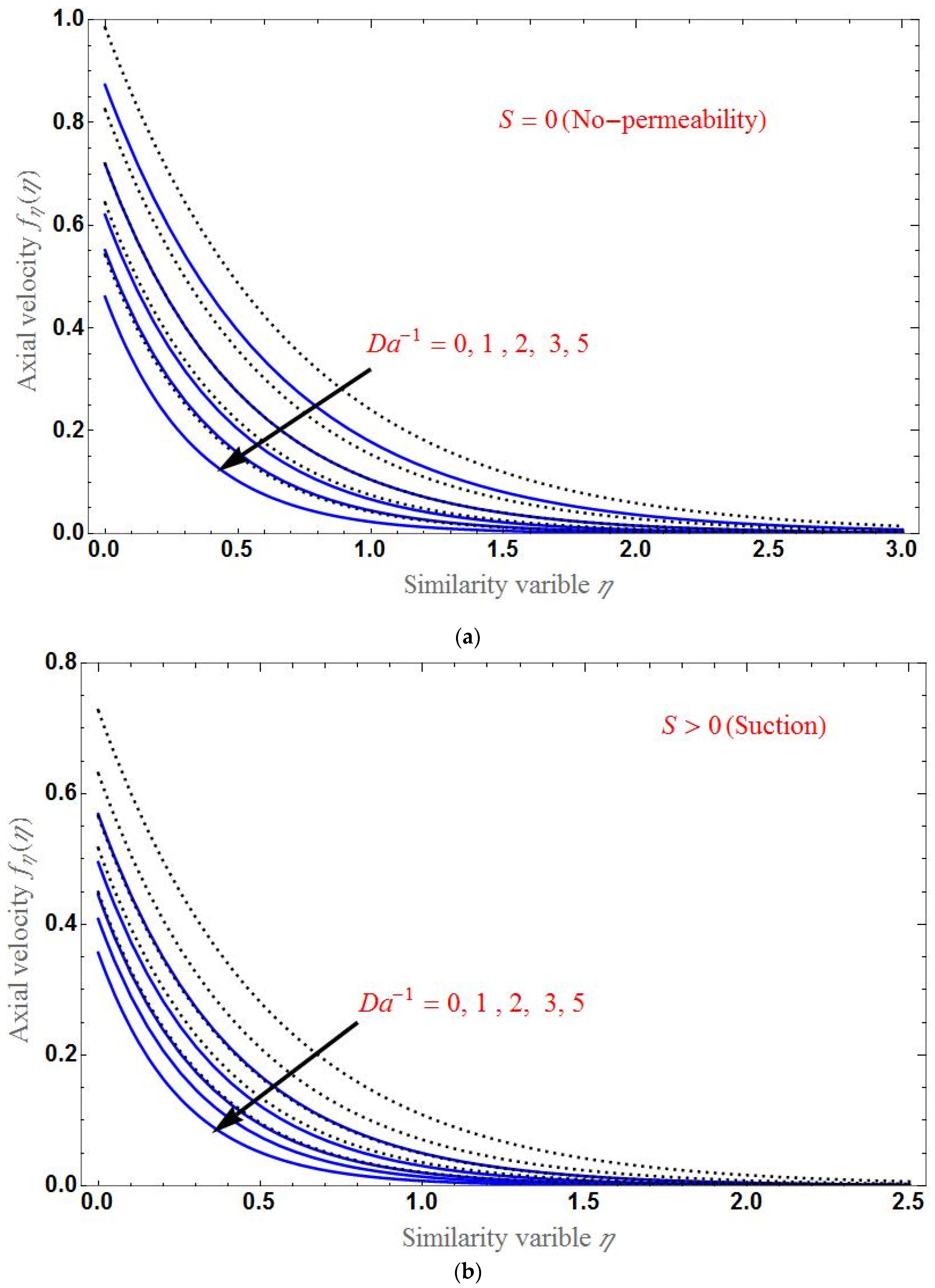
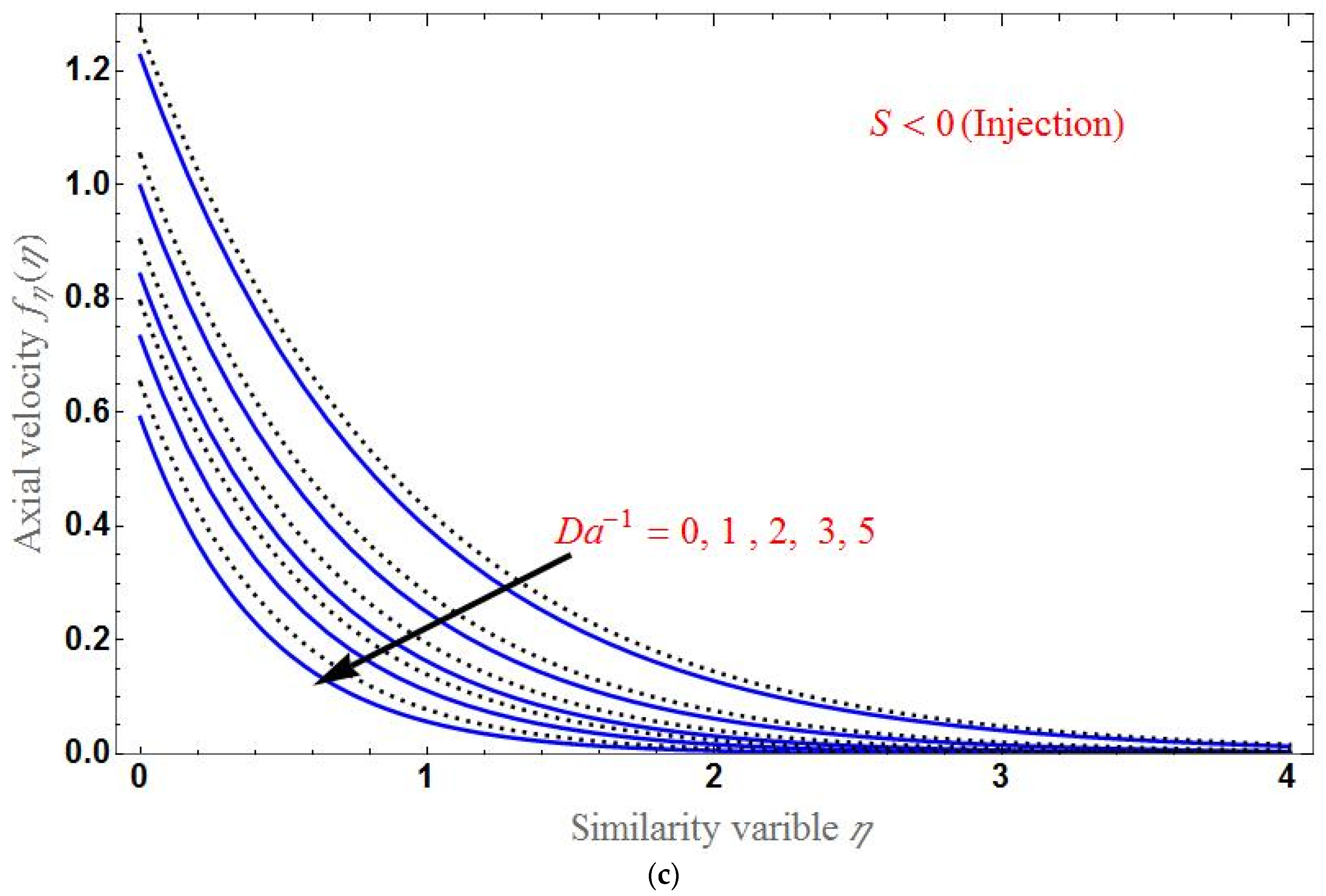
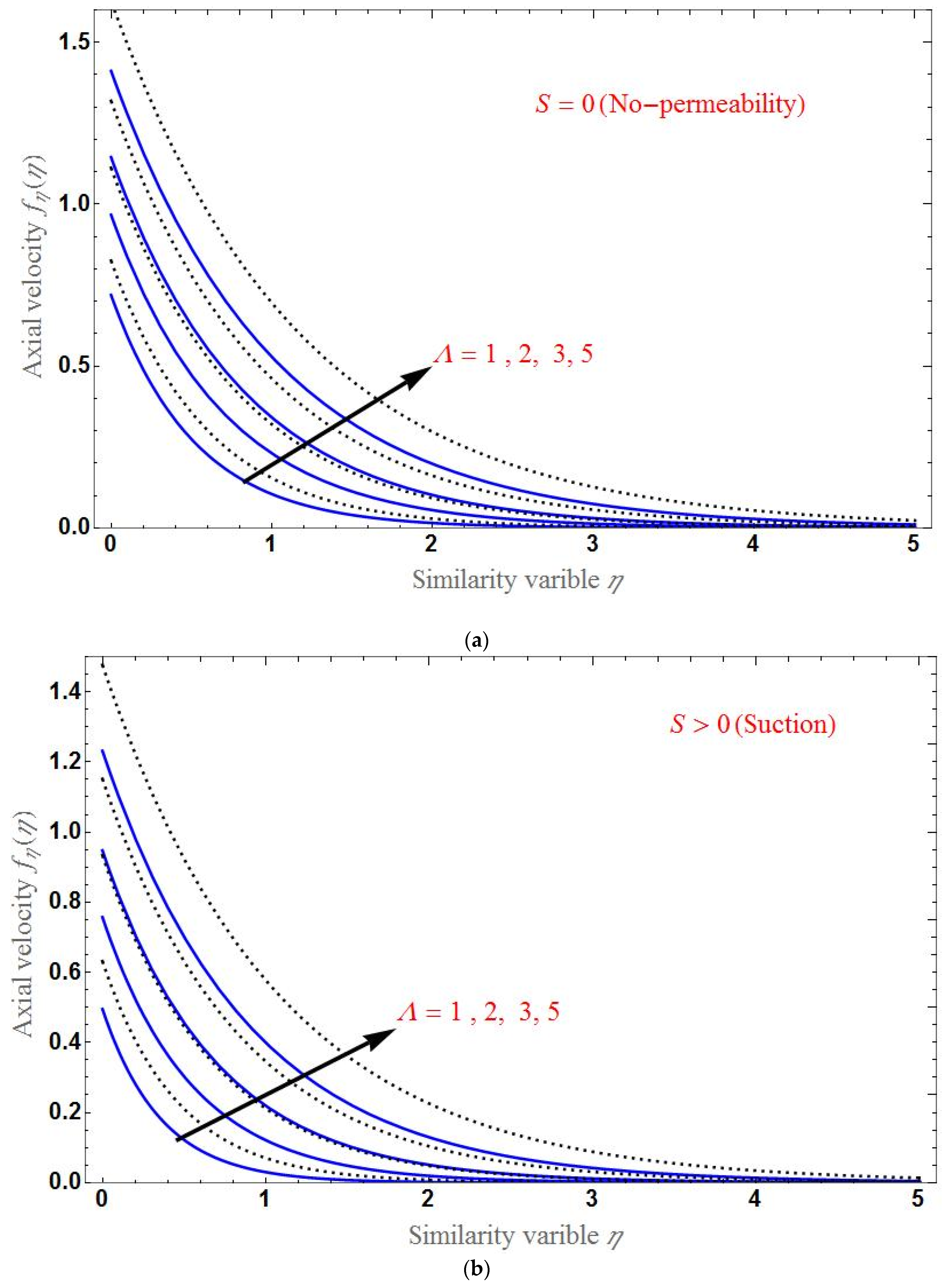
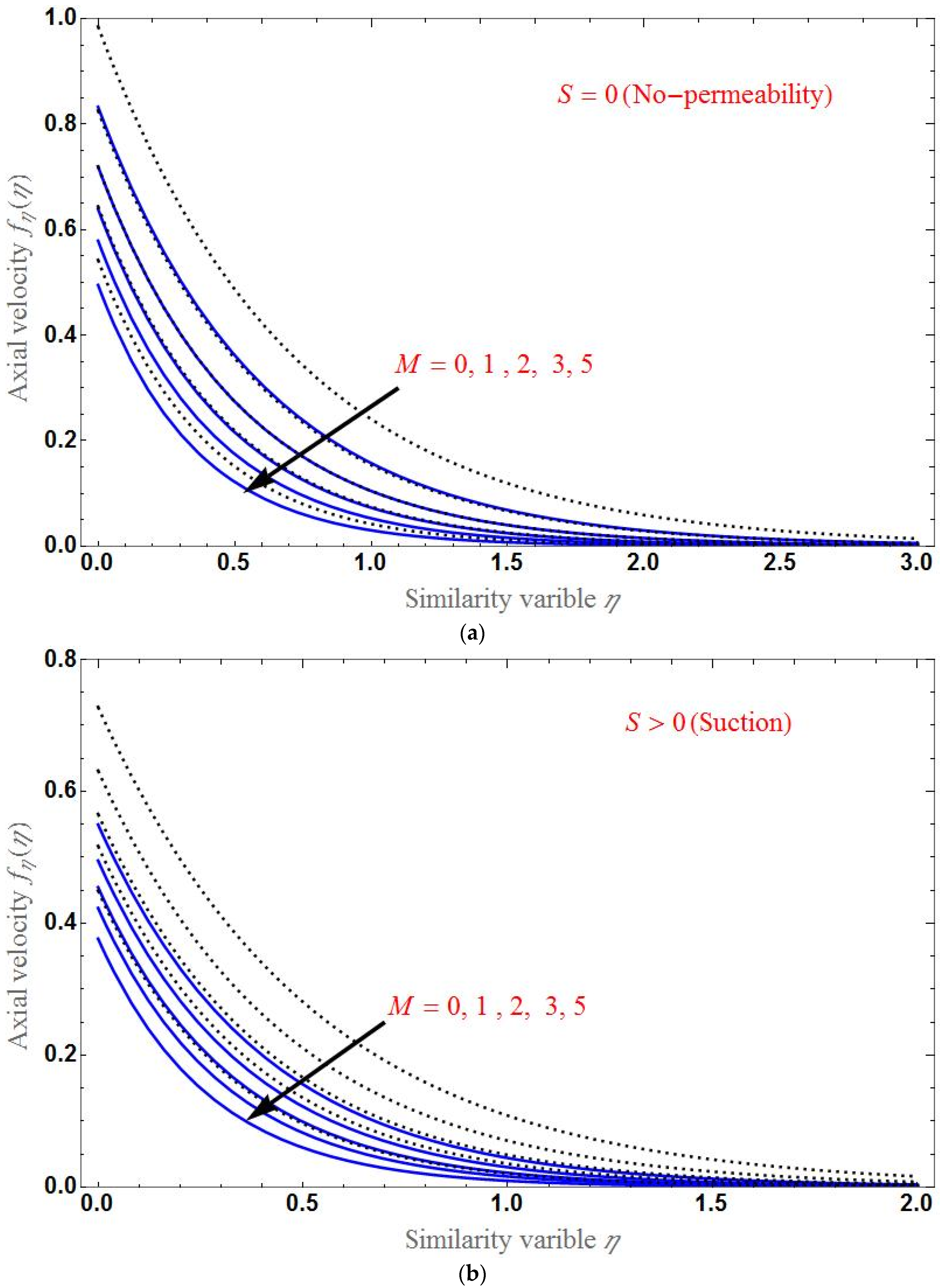
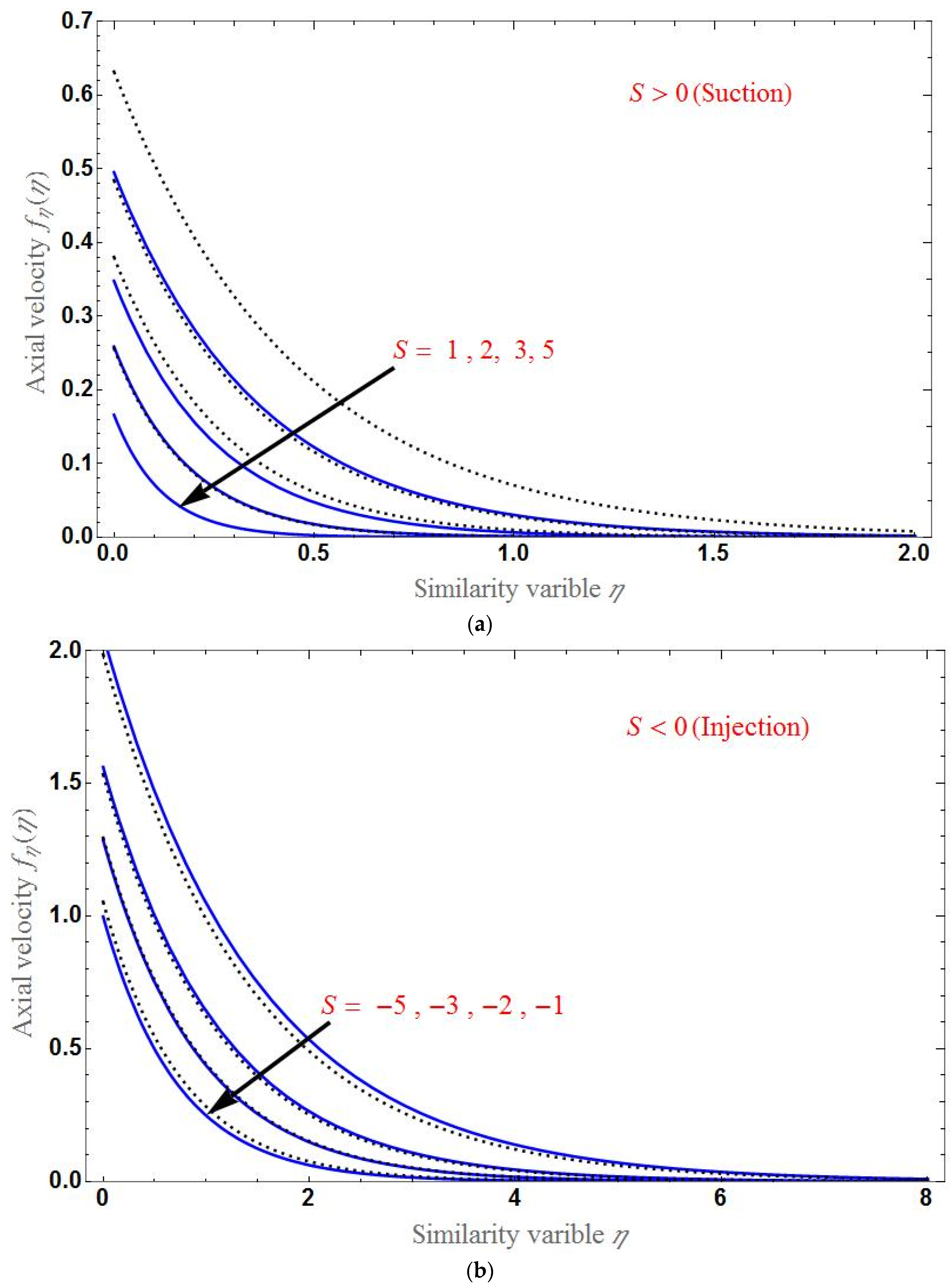
• The axial velocity declines with increasing porous parameter or magnetic field, and the suction/injection parameter increases with increasing Brinkman ratio.
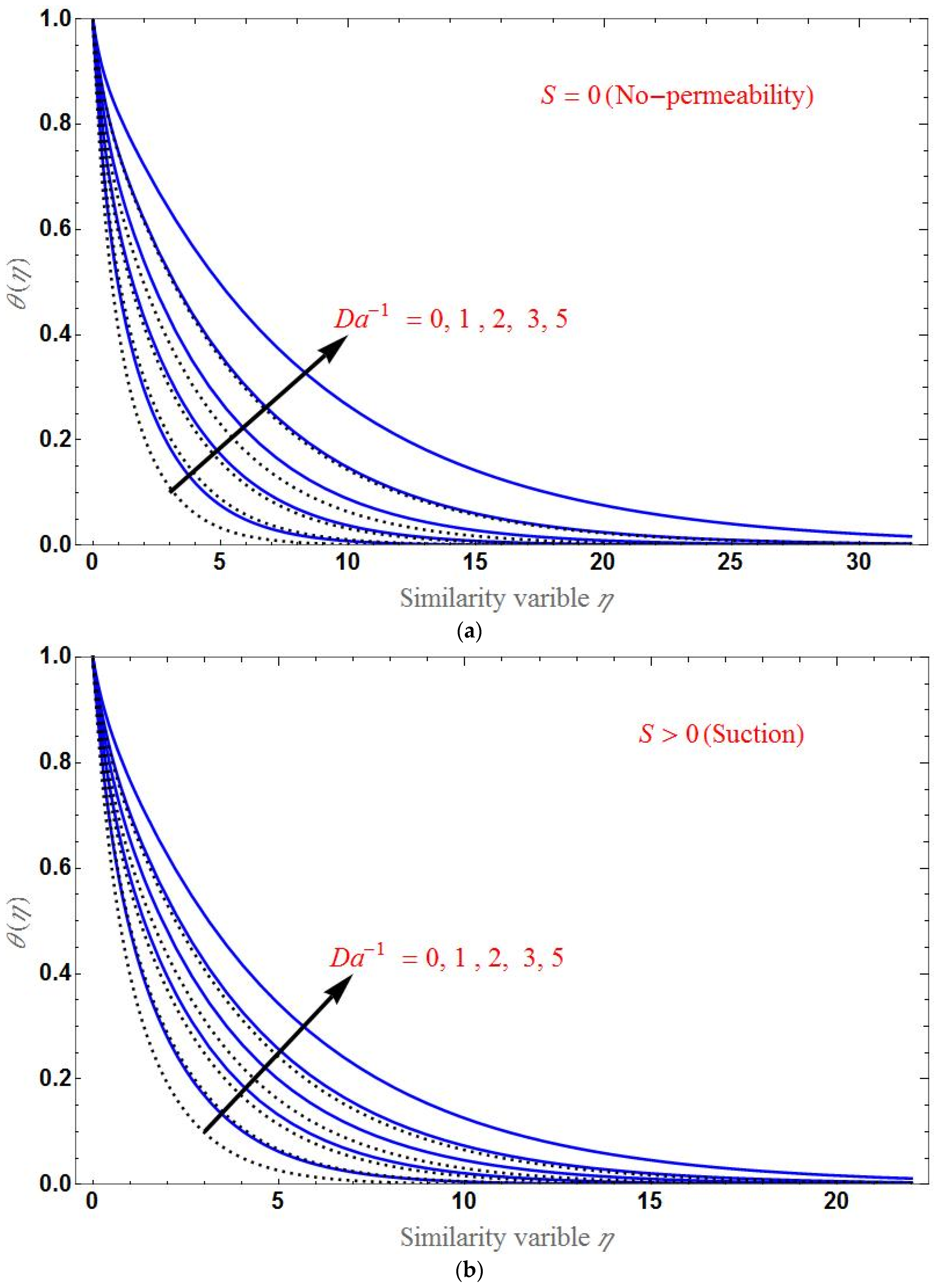
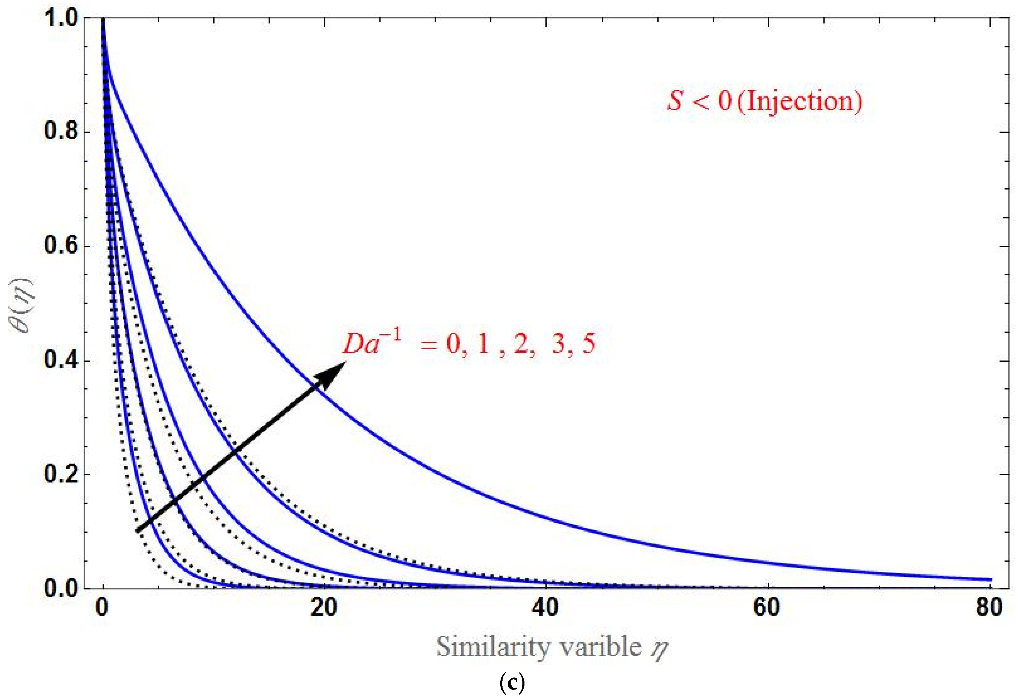
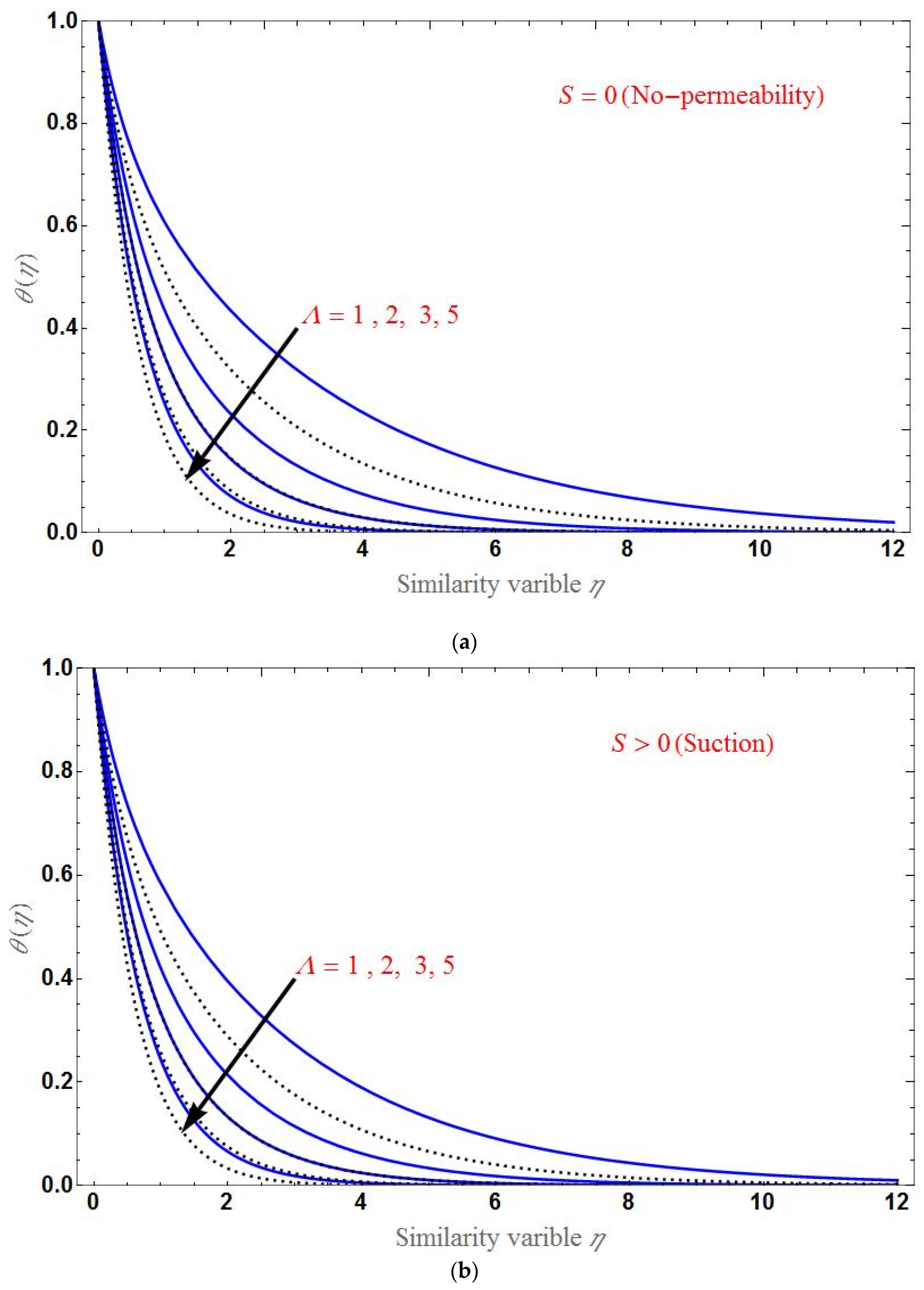
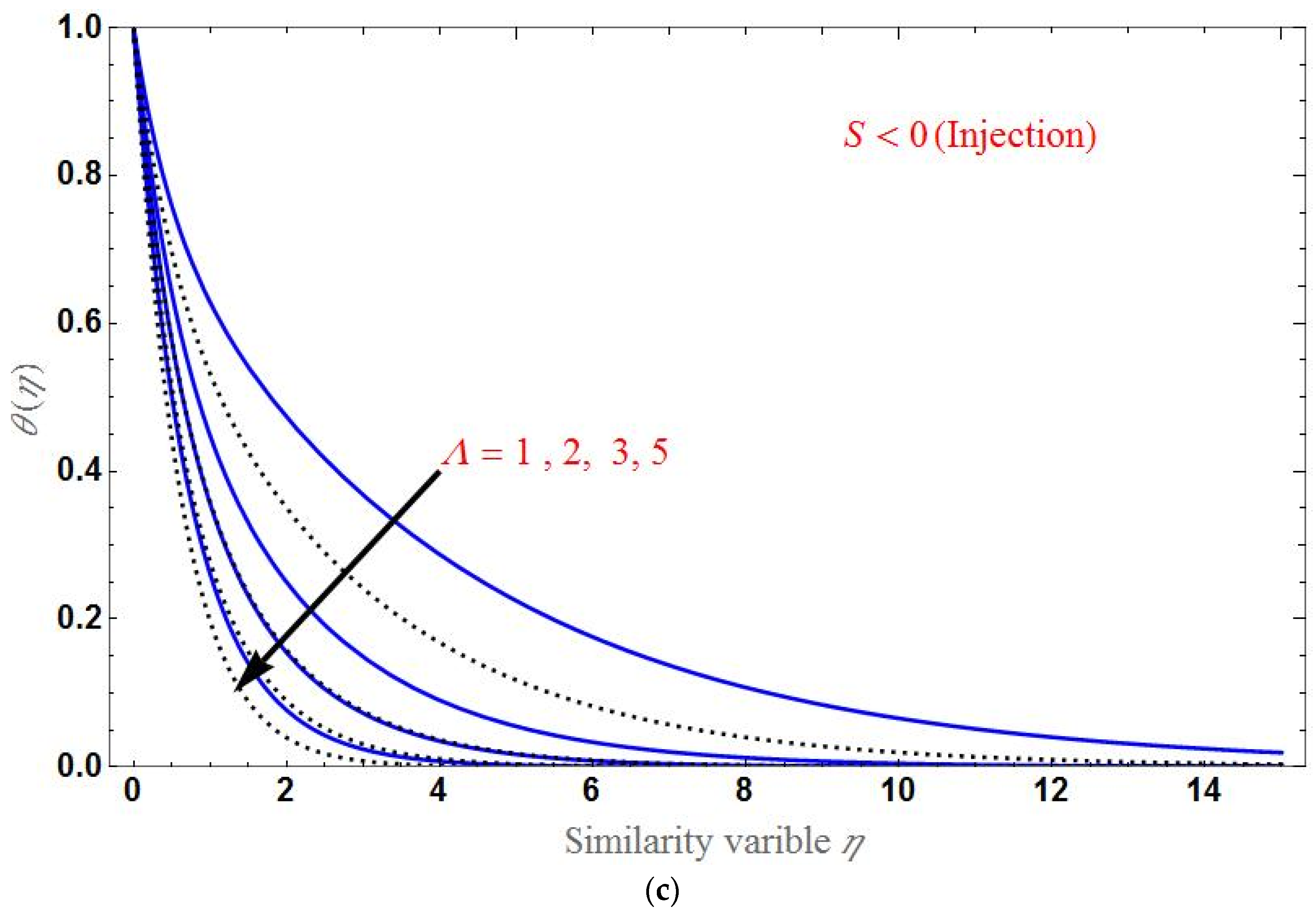
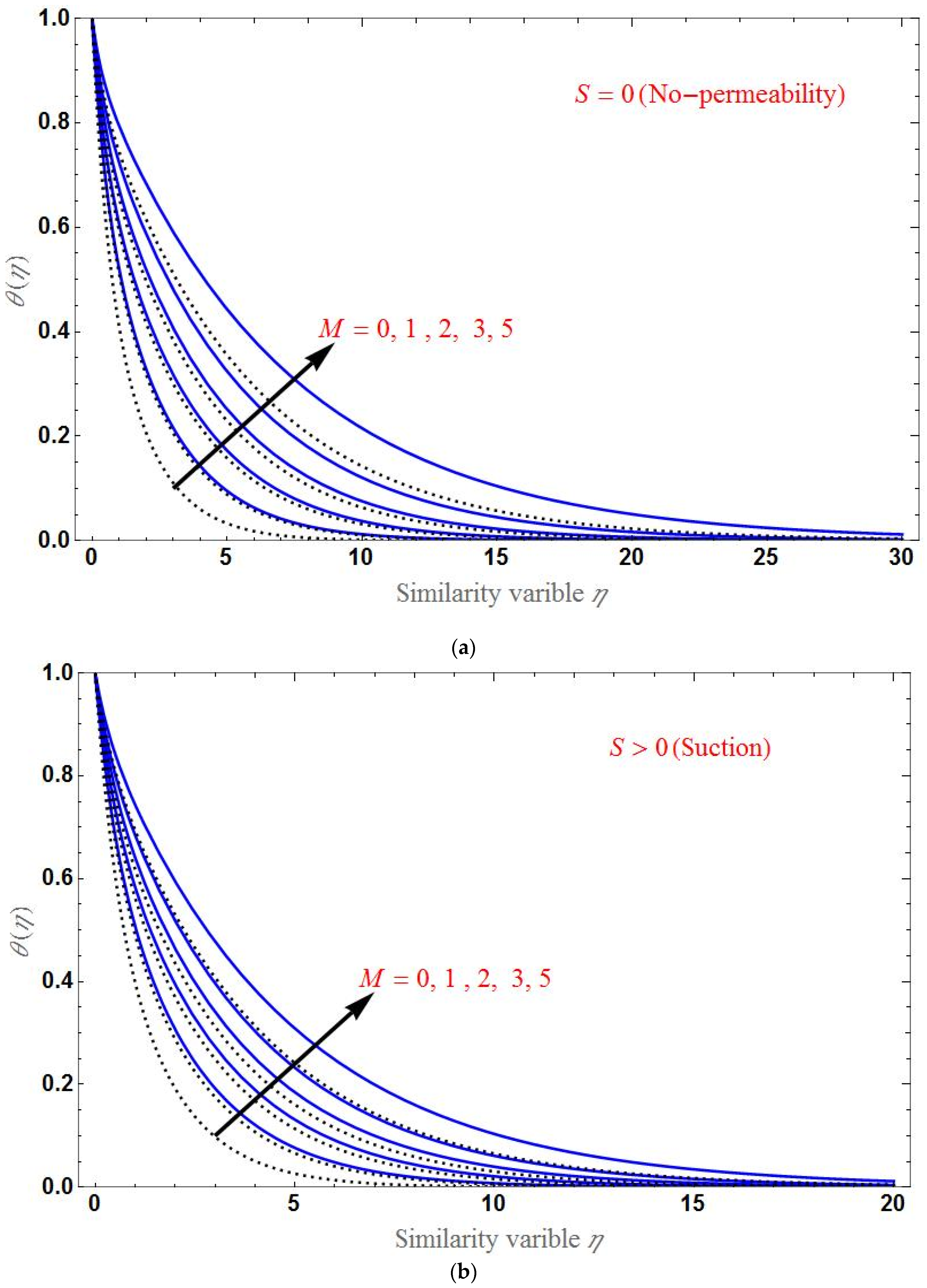
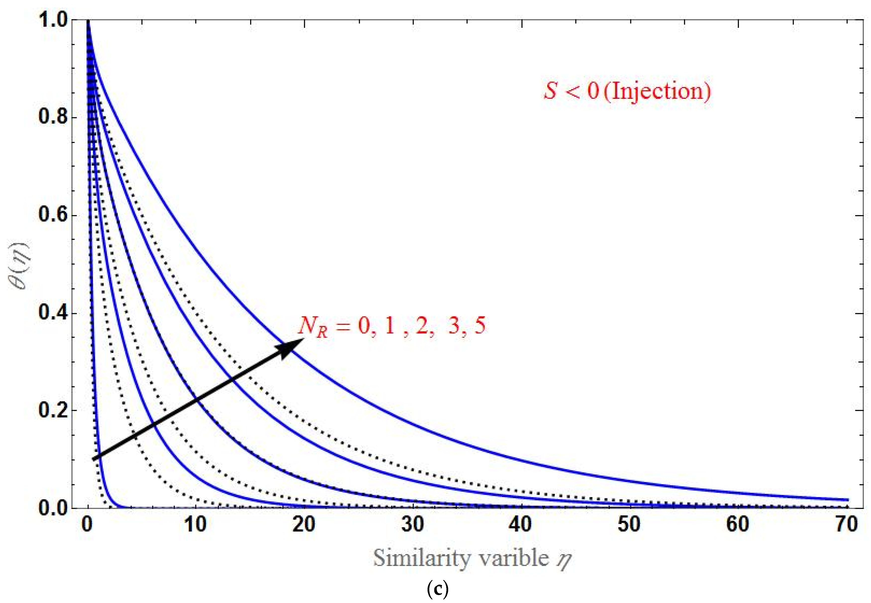
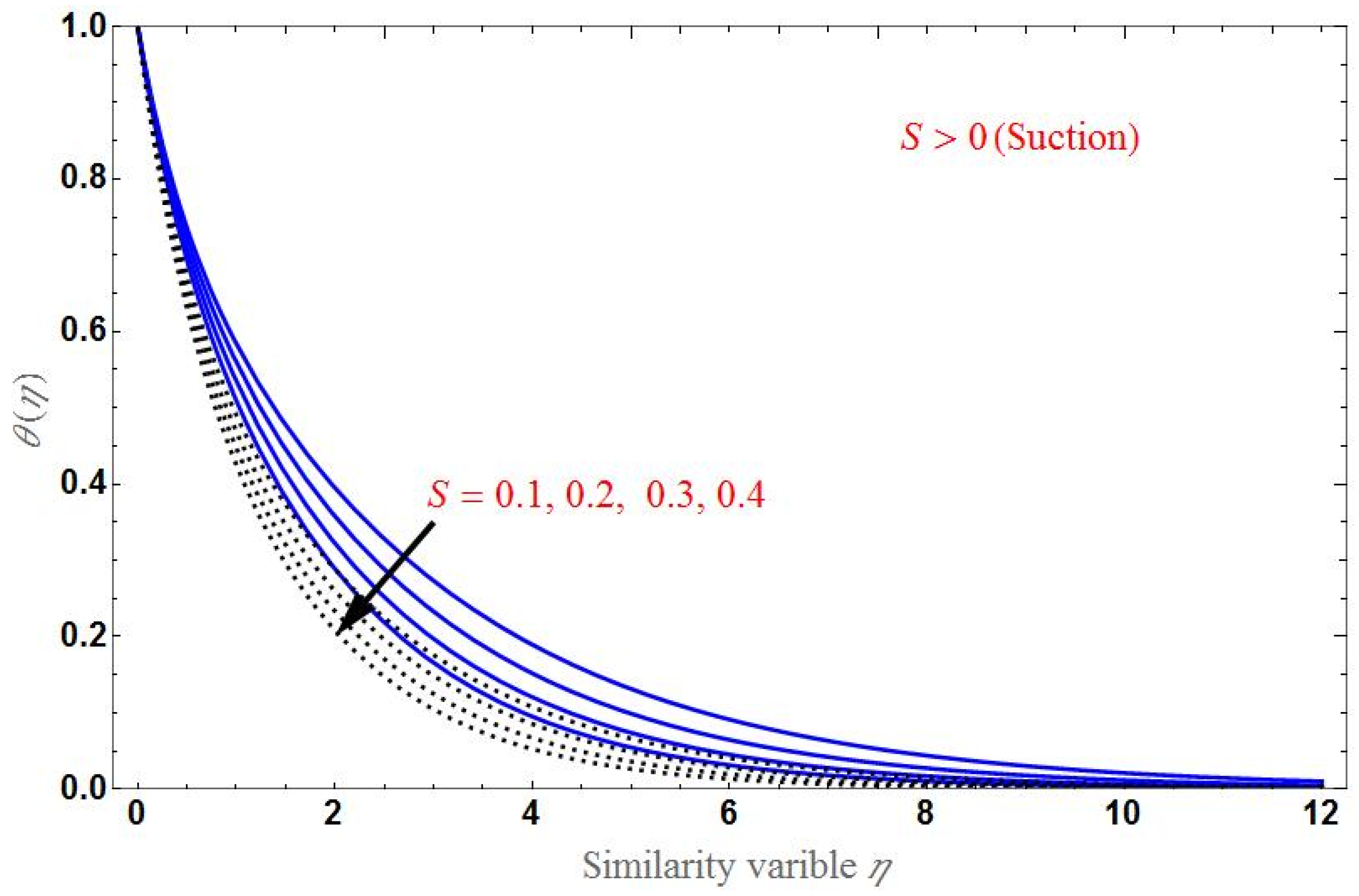
• The temperature distribution increases for higher values of the porous parameter, magnetic field, or radiation; it decreases with an increase in the Brinkman ratio or suction/injection parameter.
• At $\eta =0$, the axial velocity is different for various values of each parameter.
• The axial velocity is smaller for hybrid nanofluid than for base fluid.
• $\theta \left(\eta \right)$ is the same for every value of varying parameters at $\eta =0$.
• As the thermal rate increases upon adding nanoparticles to the base fluid, the figures showed that $\theta \left(\eta \right)$ will be larger for hybrid nanofluid than for base fluid.

In the future, we plan to conduct a similar investigation on a non-Newtonian fluid with mass transfer problems. We postulate that adding the effect of viscous dissipation and various physical parameters can uncover another interesting phenomenon.

References

- Crane, L.J. Flow past a stretching plate. Z. Angew. Math. Phys. 1970, 21, 645–647. [Google Scholar] [CrossRef]
- Wang, C.W. The three-dimensional flow due to a stretching flat surface. Phys. Fluids 1984, 27, 1915–1917. [Google Scholar] [CrossRef]
- Rosca, A.V.; Pop, I. Flow and heat transfer over a vertical permeablestretching/shrinking sheet with a second order slip. Int. J. Heat Mass Transf. 2013, 60, 355–364. [Google Scholar] [CrossRef]
- Nandy, S.K.; Mahapatra, T.R. Effects of slip and heat generation/absorptionon MHD stagnation flow of nanofluid past a stretching/shrinking surface withconvective boundary conditions. Int. J. Heat Mass Transf. 2013, 64, 1091–1100. [Google Scholar] [CrossRef]
- Kumaran, V.; Banerjee, A.K.; Vanav Kumar, A.; Pop, I. Unsteady MHD flow and heat transfer with viscous dissipation past a stretching sheet. Int. Commun. Heat Mass Transf. 2011, 38, 335–339. [Google Scholar] [CrossRef]
- Turkyilmazoglu, M. Multiple solutions of heat and mass transfer of MHD slip flow for the viscoelastic fluid over a stretching sheet. Int. J. Therm. Sci. 2011, 50, 2264–2276. [Google Scholar] [CrossRef]
- Ishak, A.; Nazar, R.; Pop, I. Unsteady mixed convection boundary layer flowdue to a stretching vertical surface. Arab. J. Sci. Eng. 2006, 31, 165–182. [Google Scholar]
- Ishak, A.; Nazar, R.; Pop, I. MHD boundary-layer flow due to a movingextensible surface. J. Eng. Math. 2008, 62, 23–33. [Google Scholar] [CrossRef]
- Ishak, A.; Nazar, R.; Pop, I. Magnetohydrodynamic (MHD) flow and heattransfer due to a stretching cylinder. Energy Convers. Manag. 2008, 49, 3265–3269. [Google Scholar] [CrossRef]
- Yacob, N.A.; Ishak, A.; Pop, I.; Vajravelu, K. Boundary layer flow past astretching/shrinking surface beneath an external uniform shear flow with aconvective surface boundary condition in a nanofluid. Nanoscale Res. Lett. 2011, 6, 314. [Google Scholar] [CrossRef] [Green Version]
- Choi, S.U.S. Enhancing Thermal Conductivity of Fluids with Nanoparticles. In Developments and Applications of Non-Newtonian Flows; Siginer, D.A., Wang, H.P., Eds.; ASME: New York, NY, USA, 1995; pp. 99–105. [Google Scholar]
- Mahabaleshwar, U.S.; Anusha, T.; Sakanaka, P.H. Suvanjan Bhattacharyya, Impact of inclined Lorentz force and Schmidt number on chemically reactive Newtonian fluid flow on a stretchable surface when Stefan blowing and thermal radiation are significant. Arab. J. Sci. Eng. 2021, 46, 12427–12443. [Google Scholar] [CrossRef]
- Mahabaleshwar, U.S.; Lorenzini, G. Combined effect of heat source/sink and stress work on MHD Newtonian fluid flow over a stretching porous sheet. Int. J. Heat Technol. 2017, 35, S330–S335. [Google Scholar] [CrossRef]
- Aly, E.H.; Pop, I. MHD flow and heat transfer near stagnation point over a stretching/shrinking surface with partial slip and viscous dissipation: Hybrid nanofluid versus nanofluid. Powder Technol. 2020, 367, 192–205. [Google Scholar] [CrossRef]
- Sarpakaya, T. Flow of non-Newtonian fluids in a magnetic field. AIChEJ 1961, 7, 324–328. [Google Scholar] [CrossRef]
- Mahabaleshwar, U.S. Combined effect of temperature and gravity modulations on the onset of magneto-convection in weak electrically conducting micropolar liquids. Int. J. Eng. Sci. 2007, 45, 525–540. [Google Scholar] [CrossRef]
- Mahabaleshwar, U.S.; Vinay kumar, P.N.; Sakanaka, P.H.; Lorenzini, G. An MHD effect on a Newtonian fluid flow due to a superlinear stretching sheet. J. Eng. Thermophys. 2018, 27, 501–506. [Google Scholar]
- Fang, T.; Zhang, J. Closed-form exact solutions of MHD viscous flow over a shrinking sheet. Commun. Nonlinear Sci. Numer. Simul. 2009, 14, 2853–2857. [Google Scholar] [CrossRef]
- Hamad, M.A.A. Analytical solution of natural convection flow of a nanofluid over a linearly stretching sheet in the presence of magnetic field. Int. Commun. Heat Mass Transf. 2011, 38, 487–492. [Google Scholar] [CrossRef]
- Turkyilmazoglu, M. Multiple analytic solutions of heat and mass transfer of magnetohydrodynamic slip flow for two types of viscoelastic fluids over a stretching surface. J. Heat Transf. 2012, 134, 071701. [Google Scholar] [CrossRef]
- Suresh, S.; Venkitaraj, K.; Selvakumar, P.; Chandrasekar, M. Effect of Al2O3–Cu/water hybrid nanofluid in heat transfer. Exp. Therm. Fluid Sci. 2012, 38, 54–60. [Google Scholar] [CrossRef]
- Suresh, S.; Venkitaraj, K.; Selvakumar, P.; Chandrasekar, M. Synthesis of Al2O3–Cu/water hybrid nanofluids using two step method and its thermo physical properties. Colloids Surf. A 2011, 388, 41–48. [Google Scholar] [CrossRef]
- Vinay Kumar, P.N.; Mahabaleshwar, U.S.; Nagaraju, K.R.; MousaviNezhad, M.; Daneshkhah, A. Mass transpiration in magneto-hydrodynamic boundary layer flow over a superlinear stretching sheet embedded in porous medium with slip. J. Porous Media 2019, 22, 1015–1025. [Google Scholar] [CrossRef]
- AmiraZainal, N.; RoslindaNazar, R.; Naganthran, K.; Pop, I. Stability analysis of MHD hybrid nanofluid flow over a stretching/shrinking sheet with quadratic velocity. Alex. Eng. J. 2020, 60, 915–926. [Google Scholar]
- Khan, U.; Shafiq, A.; Zaib, A.; Baleanu, D. Hybrid nanofluid on mixed convective radiative flow from an irregular variably thick moving surface with convex and concave effects. Case Stud. Therm. Eng. 2020, 21, 100660. [Google Scholar] [CrossRef]
- Sarkar, J.; Ghosh, P.; Adil, A. A review on hybrid nanofluids: Recent research, development and applications. Renew. Sustain. Energy Rev. 2015, 43, 164–177. [Google Scholar] [CrossRef]
- Aly, E.H.; Ebaid, A. Exact analysis for the effect of heat transfer on MHD and radiation Marangoni boundary layer nanofluid flow past a surface embedded in a porous medium. J. Mol. Liq. 2016, 215, 625–639. [Google Scholar] [CrossRef]
- Mahabaleshwar, U.S.; Nagaraju, K.R.; Vinay Kumar, P.N.; Azese, M.N. Effect of radiation on thermosolutal Marangoni convection in a porous medium with chemical reaction and heat source/sink. Phys. Fluids 2020, 32, 1136902. [Google Scholar] [CrossRef]
- Napolitano, L.G. Marangoni boundary layers. In Proceedings of the 3rd European Symposium on Material Science in Space, Grenoble, France, 24–27 April 1979. [Google Scholar]
- Chamkha, A.J.; Pop, I.; Takhar, H.S. Marangoni mixed convection boundary layer flow. Meccanica 2006, 41, 219–232. [Google Scholar] [CrossRef]
- Cortell, R. Radiation effects for the Blasius and Sakiadis flows with a convective surface boundary condition. Appl. Math. Comput. 2008, 206, 832–840. [Google Scholar]
- Mahabaleshwar, U.S.; Sarris, I.E.; Hill, A.A.; Lorenzini, G.; Pop, I. An MHD couple stress fluid due to a perforated sheet undergoing linear stretching with heat transfer. IJHM 2017, 105, 157–167. [Google Scholar] [CrossRef] [Green Version]
- Mahabaleshwar, U.S.; Nagaraju, K.R.; Vinay Kumar, P.N.; Nadagoud, M.N.; Bennacer, R.; Sheremet, M.A. Effects of Dufour and Soret mechanisms on MHD mixed convective-radiation non-Newtonian liquid flow and heat transfer over a porous sheet. Therm. Sci. Eng. Prog. 2019, 16, 100459. [Google Scholar] [CrossRef]
Publisher’s Note: MDPI stays neutral with regard to jurisdictional claims in published maps and institutional affiliations. |
© 2022 by the authors. Licensee MDPI, Basel, Switzerland. This article is an open access article distributed under the terms and conditions of the Creative Commons Attribution (CC BY) license (https://creativecommons.org/licenses/by/4.0/).
Share and Cite
Anusha, T.; Mahesh, R.; Mahabaleshwar, U.S.; Laroze, D. An MHD Marangoni Boundary Layer Flow and Heat Transfer with Mass Transpiration and Radiation: An Analytical Study. Appl. Sci. 2022, 12, 7527. https://doi.org/10.3390/app12157527
Anusha T, Mahesh R, Mahabaleshwar US, Laroze D. An MHD Marangoni Boundary Layer Flow and Heat Transfer with Mass Transpiration and Radiation: An Analytical Study. Applied Sciences. 2022; 12(15):7527. https://doi.org/10.3390/app12157527
Chicago/Turabian StyleAnusha, Thippeswamy, Rudraiah Mahesh, Ulavathi Shettar Mahabaleshwar, and David Laroze. 2022. "An MHD Marangoni Boundary Layer Flow and Heat Transfer with Mass Transpiration and Radiation: An Analytical Study" Applied Sciences 12, no. 15: 7527. https://doi.org/10.3390/app12157527
APA StyleAnusha, T., Mahesh, R., Mahabaleshwar, U. S., & Laroze, D. (2022). An MHD Marangoni Boundary Layer Flow and Heat Transfer with Mass Transpiration and Radiation: An Analytical Study. Applied Sciences, 12(15), 7527. https://doi.org/10.3390/app12157527