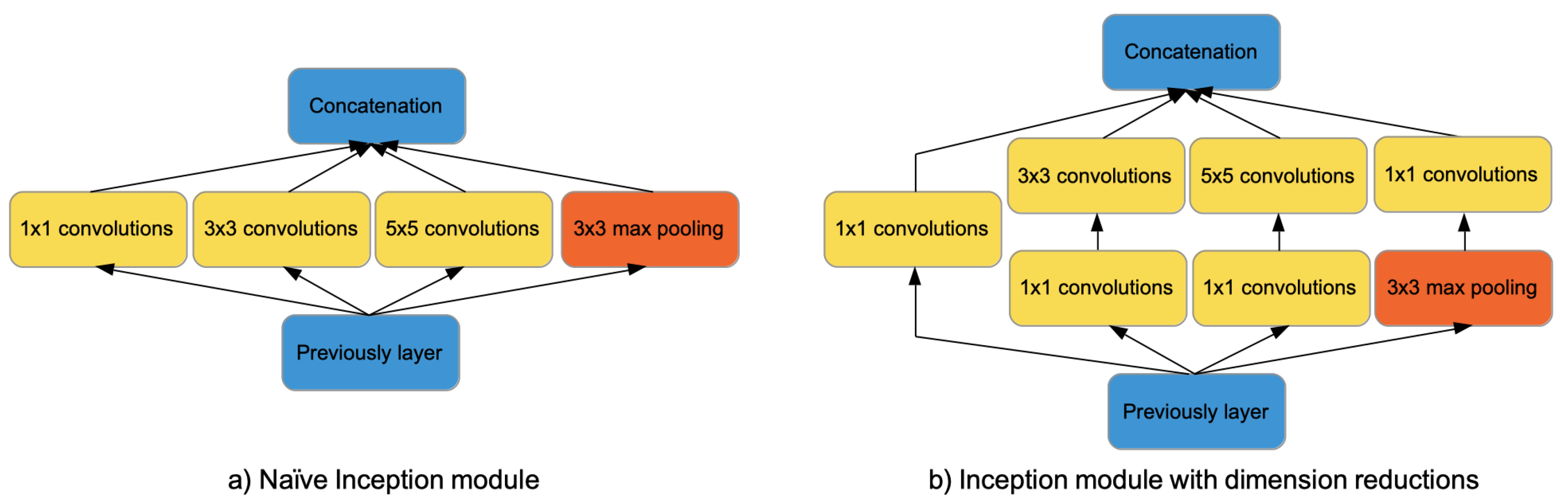
Article

A Soft-Voting Ensemble Classifier for Detecting Patients Affected by COVID-19

1
Institute of Biomedical Technologies, National Research Council of Italy, 20054 Segrate, Italy
2
Department of Mathematics and Computer Science, University of Cagliari, 09124 Cagliari, Italy
*
Author to whom correspondence should be addressed.
Appl. Sci. 2022, 12(15), 7554; https://doi.org/10.3390/app12157554
Submission received: 1 June 2022 / Revised: 15 July 2022 / Accepted: 25 July 2022 / Published: 27 July 2022
(This article belongs to the Section Computing and Artificial Intelligence)

Abstract

:
COVID-19 is an ongoing global pandemic of coronavirus disease 2019, which may cause severe acute respiratory syndrome. This disease highlighted the limitations of health systems worldwide regarding managing the pandemic. In particular, the lack of diagnostic tests that can quickly and reliably detect infected patients has contributed to the spread of the virus. Reverse Transcriptase—Polymerase Chain Reaction (RT-PCR) and antigen tests, which are the main diagnostic tests for COVID-19, showed their limitations during the pandemic. In fact, RT-PCR requires several hours to provide a diagnosis and is not properly accurate, thus generating a high number of false negatives. Unlike RT-PCR, antigen tests provide rapid diagnosis but are less accurate in detecting COVID-19 positive patients. Medical imaging is an alternative diagnostic test for COVID-19. In particular, chest computed tomography allows detecting lung infections related to the disease with high accuracy. However, visual analysis of a chest scan generated by computed tomography is a demanding activity for radiologists, making widespread use of this test unfeasible. Therefore, it is essential to lighten their work with automated tools able to provide accurate diagnosis in a short time. To deal with this challenge, in this work, an approach based on 3D Inception CNNs is proposed. Specifically, 3D Inception-V1 and Inception-V3 models have been built and compared. Then, soft-voting ensemble classifier models have been separately built on these models to boost the performance. As for the individual models, results showed that Inception-V1 outperformed Inception-V3 according to different measures. As for the ensemble classifier models, the outcome of experiments pointed out that the adopted voting strategy boosted the performance of individual models. The best results have been achieved enforcing soft voting on Inception-V1 models.

1. Introduction

COVID-19 is an ongoing global pandemic of the coronavirus disease 2019 caused by severe acute respiratory syndrome. First identified in December 2019 in Wuhan, China, the virus has spread quickly to all continents (at the time of writing, the World Health Organization is reporting around 481 million confirmed cases of COVID-19, which have caused over 6 million deaths).
Reverse Transcriptase—Polymerase Chain Reaction (RT-PCR) and antigen tests are the main diagnostic tests for COVID-19. During the pandemic, RT-PCR has shown its limitations in detecting COVID-19. On the one hand, the performance of this diagnostic test reported a low sensitivity, resulting in a large number of false negatives. On the other hand, RT-PCR is a laboratory technique that requires several hours to provide a diagnostic result. Unlike RT-PCR, antigen tests provide quick diagnoses, but they have a lower sensitivity with respect to that of RT-PCR [1]. A fast and accurate diagnostic test would allow both to quickly isolate infected patients limiting the spread of the virus and to promptly provide them with the first targeted treatments.
Diagnostic imaging is an alternative approach aimed at detecting COVID-19 infections. In particular, chest scans obtained with computed tomography (CT) allow accurately detecting lung abnormalities due to COVID-19, together with the possibility of identifying lesions that explain the degree of severity of the disease. Unfortunately, a diagnosis can only be made by analyzing a multitude of chest slices obtained through a scan. Moreover, recognizing lung infections related to COVID-19 is not trivial. Although the CT findings of COVID-19 are well known [2], it can be difficult to properly differentiate COVID-19 from other kinds of viral pneumonia. A targeted study involving radiologists in China and the United States of America showed how their performance was characterized by a moderate sensitivity in distinguishing COVID-19 from viral pneumonia [3]. Therefore, it is essential to support radiologists with automated tools able to analyze CT scans and targeted to provide accurate COVID-19 diagnosis in a short amount of time.
Deep learning (DL) can be successfully used to implement algorithms able to deal with this challenge. DL has rapidly become a methodology of choice in diagnostic imaging [4]. It is increasingly used to analyze medical images in different fields obtained with different medical imaging tools (e.g., [5,6,7]) including CT (e.g., [8,9]). Some DL-based solutions have also been proposed to detect COVID-19 lung infections. With no claim to be exhaustive, some works are reported hereinafter. For the screening of COVID-19, Silva et al. [10] proposed a method based on EfficientNet [11] that adopts transfer learning and a voting-based approach. In particular, the 2D images of a chest CT scan from a given patient are classified as a group in a voting system. In [12], the authors proposed CovNet19 to predict COVID-19 by analyzing chest X-ray images. CovNet19 uses pre-trained Convolutional Neural Networks (CNNs) for feature extraction and a Support Vector Machine (SVM) [13] for classification. In [14], Zhang et al. proposed a system consisting of a cascade of two models: a lung-lesion segmentation model and a diagnostic model. The former is used to generate a lung-lesion map, which is given as input to the latter. The diagnostic model classifies scans as related to novel coronavirus pneumonia, common pneumonia and normal controls. A similar approach aimed at classifying COVID-19, SARS, and MERS chest X-ray (CXR) images using CNNs is presented in [15]. A unique dataset representative of the three infections was compiled and used as a benchmark for the study. Then, a two-level recognition system was implemented. In the first step, the lung regions are segmented, while in the second step, a CNN is used to classify the segmented regions. In [16], the authors proposed a system to perform lung segmentation, COVID-19 diagnosis, and COVID-19 infections slices locating. The diagnostic network was able to process 2D images and to classify input slides into five categories, i.e., non-pneumonia, community-acquired pneumonia (CAP), influenza-A, influenza-B, and COVID-19. Li and Li [17] proposed a deep learning voting approach combining multiple CNNs to detect COVID-19 by analyzing chest X-ray images. Transfer learning was used to build 17 models. Then, the outcome obtained by these models is combined using a majority voting rule. The built model is able to distinguish patients affected by COVID-19 from those with bacterial pneumonia or without pneumonia. Transfer learning has been also used in [18]. In this work, the authors used transfer learning on residual networks (i.e., ResNet-50) to detect COVID-19 positive patients from 2D chest CT images. A novel model called deep contrastive mutual learning (DCML) for COVID-19 recognition was proposed in [19]. In this work, to avoid the overfitting, the training set was enriched using a multi-way data augmentation strategy based on the Fast AutoAugment algorithm [20]. Then, the contrastive learning was combined with the conventional deep mutual learning (DML) framework to obtain more discriminative image features through a new adaptive model fusion method. The interested reader can find an outline of the current state-of-the-art of COVID-19 image classification in [21].
This work addresses the issue of detecting COVID-19 infections by analyzing chest CT scans with 3D Inception-based models, with the goal of identifying patients with no infections, affected by common pneumonia, and affected by COVID-19 pneumonia. To this end, first, individual models have been trained starting from 3D Inception-V1 and Inception-V3 CNNs; then, the voting ensemble method has been experimented with to improve their performance. The comparative setting in which experiments have been carried out includes the individual models and the ensembles. Experimental results have also been compared with those obtained by other works proposed in the literature.
The remainder of this article is organized as follows. First, materials and methods are described; then, experiments and the corresponding results are presented. A discussion on the results and on the challenges that arise from this classification task follows. Finally, conclusions are drawn.

2. Materials and Methods

As CT scans can consist of hundreds of slices, training DL models able to analyze this huge amount of data is a challenging task. Independently from the specific problem, two main approaches based on analyzing 2D or 3D images have been proposed in the literature.
The first approach is twofold, as one or more representative slices of a scan can be analyzed. In the former case, no further work is required, whereas in the latter, each slice is analyzed independently, and then individual results are combined to produce the desired outcome. In the second approach, a subset of the available slices is selected and analyzed together. Basically, the first approach requires less memory and is computationally less expensive than the second, but information about chest slices contiguity is lost. The proposed work is based on the latter approach.
A soft-voting ensemble approach built on Inception networks able to analyze 3D images to detect COVID-19 infections is proposed. Inception networks have been used for their ability to limit overfitting when working with not large datasets. Moreover, the size of these networks allowed fitting the trainable 3D model on the device memory according to different settings. Details of the materials and the implemented methods are reported in the following.
This section is organized as follows: first, the Inception-based architectures used in this work are recalled; then, a brief summary of the main ensemble classifier methods is given; afterwards, the dataset used to train and test the models is described; and finally, the strategy adopted for dealing with the detection of COVID-19 is presented.

2.1. Inception Networks

CNNs are a class of deep neural networks widely used for images analysis. Basically, a CNN implements a stack of several modules that perform convolutions, introduce non-linearity to the model, downsample the features and classify the images. These operations make use of convolutional, ReLU, pooling, and fully connected layers. The convolutional layer represents the core building block of a CNN. It applies a set of convolution filters to the input feature map, producing an output feature map. Optimal values for the filters are learned by the CNN during the training phase. The ReLU layer is used to apply the rectifier function, with the aim of increasing the model’s non-linearity after convolution. The pooling layer is used to downsample the features by implementing a dimensionality reduction of the feature map. Finally, the fully connected layer performs the classification task using the features extracted by the previous layers.
Inception networks represented a milestone in CNNs. Before the advent of Inception, the design of CNN architectures was focused on increasing the convolutional layers. However, networks designed according to this principle have some limitations. In particular, the number of parameters of the network increases with the number of network layers. As a consequence, the parameters might not fit in memory. Moreover, models built on very deep networks can be affected by overfitting, especially when working with not large datasets. To deal with these limitations, Inception moved from fully connected network architectures to sparsely connected network architectures. This idea resulted in the so-called Inception module. The naïve Inception module consists of a pooling path and filters of different sizes (i.e., 1 × 1, 3 × 3, 5 × 5) which perform convolutions on the input image (see Figure 1a). The output generated by these operators is concatenated into a single output vector representing the input of the next layer. Some convolutions can become prohibitively expensive on top of a convolutional layer with a large number of filters. To deal with this issue, the Inception module has been modified by adding 1 × 1 convolutions to compute reductions before the expensive 3 × 3 and 5 × 5 convolutions (see Figure 1b). This Inception module has been used to build the so-called Inception-V1 network [22] consisting of 27 layers.
Inception-V2 and Inception-V3 are two incremental optimizations presented in the same paper [23]. Architectural changes implemented in Inception-V2 are aimed at reducing the computational cost with respect to Inception-V1. This was obtained implementing smart factorization methods aimed at making convolutions computationally more efficient. In Inception-V2, convolution filters with kernel size 3 × 3 were factorized to two 5 × 5 convolutions. This change affects the performance of the network in terms of computational time and accuracy. Notably, a 5 × 5 convolution is 2.78 times more expensive than a 3 × 3 convolution. Moreover, using 3 × 3 is preferable to larger kernel size, which may affect the accuracy of a neural network due to the representational bottleneck. Additionally, n × n convolutions were factorized to a stack of 1 × n and n × 1 convolutions (see Figure 2). Converting 3 × 3 convolutions into 1 × 3 and 3 × 1 convolutions was 33% cheaper in terms of computational cost.
Inception-V3 implements all changes reported for Inception-V2 and additionally makes use of (i) RMSprop optimizer, (ii) label smoothing regularization, (iii) 7 × 7 factorized convolution, and (iv) batch normalization in the fully connected layer. Experiments carried out in the paper presenting both architectures showed that better performances were obtained using Inception-V3 also outperforming Inception-V1.

2.2. Ensemble Classifiers

Ensemble methods are machine learning solutions aimed at building a more robust and effective model starting from a group of base models (say “base” or “weak” models). As long as certain requirements are met (e.g., enforcing diversity), an ensemble typically performs better than its base models. Note that there are no general constraints on the technology used to generate the base models, meaning in particular that it is not required for them to be homogenous.

2.2.1. Training Strategies for Ensemble Methods

As for training strategies, ensemble methods fall in two categories, namely sequential and parallel.
Sequential ensemble methods—The base models are built in a pipeline, with the goal of progressively improving the performance of the ensemble. At each step, the current solution is typically refined by adding a new base classifier biased toward the residual misclassification errors. Boosting algorithms are the most well-known sequential ensemble methods, in which any new base model is forced to focus on misclassified examples, assigning them a higher probability of being selected as part of the current training set.
The interested reader may consult [24] to obtain a deeper insight into the capability of boosting methods to improve the overall performance in a residual-decreasing way.
Parallel ensemble methods—Since combining base models that make independent classification errors can significantly improve the overall performance, base models are trained in parallel, and their independence in misclassification errors is fostered with various techniques. Bagging algorithms are well-known representative for parallel ensemble methods. By construction, bagging is aimed at generating an ensemble that shows a lower variance on errors with respect to the base classifiers. In particular, a set of independent models is obtained from different training sets built by using bootstrap sampling [25].

2.2.2. Blending Policies for Ensemble Methods

In principle, training strategies and blending policies are independent of each other, whereas in practice, there is often a bias toward a specific output blending policy given the adopted training strategy. Some the most acknowledged voting policies are introduced hereinafter, which are followed by relevant comments on their use with sequential and parallel ensemble methods.
Given an instance to be classified, several base classifier outputs must be blended together to give rise to the actual classification. Voting and stacking are the main blending methods acknowledged by the research community.
Voting—Two main voting policies are feasible, namely hard and soft voting (see Figure 3).
A schematic representation of both concepts follows hereinafter. Let m i be the i-th model of an ensemble consisting of N individual classifiers aimed at predicting the class label from a set of k possible labels { c 1 , c 2 , , c k } . For a given input x, the classifier m i will generate a k-dimensional vector [ m i 1 ( x ) , m i 2 ( x ) , , m i k ( x ) ] , where m i j ( x ) is the output of the i-th model for the j-th category label. All N individual classifiers are treated equally, and the overall classification is obtained by averaging the individual outputs with varying the class label and then selecting the label k * corresponding to the highest vote. In symbols:
k * = arg max j M j ( x ) = arg max j 1 N · i = 1 N m i j ( x ) = arg max j i = 1 N m i j ( x )
Note that the above formula can be adapted to both hard- and soft-voting policies, depending on whether base classifiers output a value in { 0 , 1 } (hard voting) or in [ 0 , 1 ] (soft voting). In the former case, majority voting is actually enforced, meaning that the class that obtained most votes by the base models is selected, whereas in the latter case, m i j ( x ) represents an estimate of the posterior probability P ( c j | x ) issued by the i-th base classifier.
Weighted voting can be seen as a generalization of the previous cases, as here, base models are combined depending on a weight that accounts for their importance. Under the same hypotheses made above, and assuming that w i represents the weight assigned to the i-th model m i , the weighted voting policy can be summarized as follows:
k * = arg max j M j ( x ) = arg max j i = 1 N w i · m i j ( x )
Note that weighted voting is the most general case of voting, as non-weighted voting can be easily simulated by setting each individual w i to any given positive constant (e.g., w i = 1 ).
Stacking—An ensemble made of base models can also be combined by training a meta-learner. The obtained model will output a prediction starting from those of the base models. There are no constraints on the type and technology of the stacking module, which in particular is not tied to the type of base classifiers.

2.3. Dataset Used for Experiments

The study is based on the China Consortium of Chest CT Image Investigation (CC-CCII) dataset [14]. CC-CCII is a large dataset built collecting chest CT scans from six hospitals in China. It consists of 408,350 slices obtained from 4167 scans. The dataset includes chest CT scans from patients affected by both novel corona virus pneumonia (NCP) and common pneumonia (CP) as well as from normal controls (Normal) (see Table 1). As reported in the table, CC-CCII is an imbalanced dataset. NCP and CP instances are equally represented, whereas Normal instances represent the minority class. As for the CP group, it consists of CT scans from patients affected by viral, bacterial, and mycoplasma pneumonia. Chest CT scans were obtained using a window width of 1200 and window center of −600, and the slices of size 512 × 512 were converted from Hounsfield Units (HU) values to grayscale. The dataset is released as a set of ordered PNG images representing the slices of each CT scan.
To the best of our knowledge, CC-CCII is the largest publicly available dataset and the only one classifying the scans according to the before described classes. However, CC-CCII comes with some issues. As highlighted in [26], CC-CCII contains damaged data, non-unified data type, repeated and noisy slices, disordered slices, and non-segmented slices. In the same work, the authors addressed these issues releasing CLEAN-CC-CCII, a cleaned version of the CC-CCII dataset, consisting of 340,190 slices from 4023 scans (see Table 2).
In particular, in CLEAN-CC-CCII:
  • Damaged data have been removed. This consists of around 10% of the CC-CCII downloadable zip files that cannot be successfully decompressed;
  • All slice image files have been unified to the PNG format without losing the information of the original files;
  • Duplicated slices have been manually removed to avoid redundant data by scanning all the images in CC-CCII;
  • All scans of CC-CCII have been analyzed to rearrange the disordered slices to the correct order;
  • An open-source K-Means-based method has been used to segment lungs from the CT slices and remove the white background.
As the issues identified in CC-CCII may impact the training phase of a model, in this work, the cleaned dataset CLEAN-CC-CCII has been used.

2.4. The Proposed Approach

The pipeline aimed at training and testing both the individual models and the soft-voting ensemble models is graphically represented in Figure 4. Summarizing, its first step is aimed at pre-processing the chest CT dataset. Specifically, the dataset has been pre-processed to uniform the depth of the CT scans and to remove irrelevant contents for the problem in hand. Then, with the aim of reporting an accurate estimate of the models’ prediction performance, the dataset has been split to implement a 5-fold cross-validation. Subsequently, five individual models have been independently built, tuning a hyperparameter of the network. To avoid overfitting, an online image augmentation process has been enforced while training the networks. Performances of each model have been independently assessed according to the 5-fold cross-validation. Then, the soft-voting ensemble models have been built using the individual models. Details of these steps are described in the following.

2.4.1. Data Pre-Processing

The dataset used in this work consists of CT scans with slices of 512 × 512 pixels and a non-uniform depth size. Therefore, it has been necessary to process the scans so that each of them has the same depth size. This was also completed with the aim to assess how the scan depth affects the classifier’s performance. To this end, the CT scans in the CLEAN-CC-CCII dataset were processed to generate two sets of scans with two distinct depth sizes. These sets consisted of CT scans with a uniform depth size of 25 and 35 slices.
This pre-processing step has required to down-sample or over-sample the CT scans according to their original depth. The adopted strategy to perform these operations was to work at the ends of the scans, where generally, the information content is lower (see Figure 5). Basically, the oversampling was implemented by replicating the slices at both ends. Similarly, the downsampling was implemented by removing the slices starting from the ends.
In addition, the size of the slices had to be reduced to meet the memory constraints of the GPU. To this end, the central part of each slice has been cropped with a fixed size and then scaled to 256 × 256 pixels (see Figure 6). The cropping has been aimed at removing contents non-informative for the problem at hand but that might affect the training phase.

2.4.2. Training

Models have been built to be able to classify a 3D CT according to three possible classes (i.e., Normal, NCP and CP). For the aim of this work, Inception architectures adapted to analyze 3D inputs have been used. Due to the adopted testing strategy, i.e., 5-fold cross-validation, at each step, the dataset is automatically split into training (80%) and testing (20%). Each model has been trained with 2896 CT scans—note that 80% of 4023 scans amounts to 3218, but only 90% are used for training, whereas 10% are used for validation (see Table 3).
Given a scan, to fit the GPU memory, only a fixed number of the available slices (i.e., 25 and 35) has been used to represent each sample. In particular, the number of features (observed variables) relating to each scan amounts to 1,638,400 (i.e., 256 × 256 × 25) when taking 25 slices, whereas 2,293,760 (i.e., 256 × 256 × 35) features are required when taking 35 slices.
It should be pointed out that working with an overwhelming number of features with respect to the available observations raises the well-known curse of dimensionality issue, which was first introduced by Bellman [27]. In particular, as the total amount of features increases, overfitting becomes more and more likely. To limit the overfitting, image augmentation has been enforced.
Let us recall that image augmentation refers to techniques used to increase the amount of images in a dataset. Basically, it applies transformations (e.g., flipping, shifting, rotating) to existing images with the aim to create modified copies of them. In DL, image augmentation is applied with a twofold aim. In particular, it allows increasing the amount of data used to train a deep network with the aim of preventing overfitting. Moreover, the level of variation embedded with the new images allows building more robust models, enabling better generalizing on unseen images.
Image augmentation can be implemented offline or online. In the former case, the transformations are applied before the learning process starts. In the latter case, augmentation is performed at each epoch, typically injecting some randomness in the procedures used for augmentation. As a consequence, whereas the offline approach generates a fixed set of augmented scans, the online approach generates augmented CT scans that in principle are different at each epoch.
The online image augmentation approach has been used in this work. Basically, at each epoch, the CT scans have been modified by slightly rotating and shifting them. For each CT scan, the rotation and shift factors were randomly generated and applied to all slices.

2.4.3. The Ensemble Model Classifier

As previously mentioned, the proposed approach uses an ensemble method to boost the performance of a set of estimators. In particular, a soft-voting strategy has been applied and assessed on ensembles of Inception-V1 and Inception-V3 models. It should be pointed out that generally, soft voting is applied to homogeneous ensembles. For heterogeneous ensembles, the class probabilities generated by different type of learners cannot be compared directly without a careful calibration [24]. Starting from this consideration, ensemble classifier models have been separately built on Inception-V1 and Inception-V3.
The individual models have been built tuning a single hyperparameter of the networks. Each model has been built to be able to analyze a 3D CT scan to generate a distribution probability according to three possible classification labels (i.e., Normal, NCP and CP) (see Figure 7).
Then, the ensemble classifier model combines the output of each individual model through a decision fusion layer to provide the final output (see Figure 8). In particular, each ensemble consists of five models obtained tuning the dropout value of the last (fully connected) layer of the networks. Dropout [28] refers to a technique to prevent overfitting issue in neural networks. Basically, it works by ignoring a set of randomly selected neurons during the training phase. In so doing, it forces a neural network to learn more robust features that are useful in conjunction with many different random subsets of the other neurons [29]. The hyperparameter used to control the dropout is used to specify the probability that neurons at a given layer are dropped. The five models of each ensemble have been built setting this hyperparameter to 0.0 and ranging it from 0.3 to 0.6 with a step size of 0.1.

3. Results

Experiments have been carried out to assess the proposed approach according to different aspects. Specifically, they have been designed to (i) compare Inception-V1 and Inception-V3 architectures for the problem at hand, (ii) compare the performance of individual models with respect to ensemble models, and (iii) assess if the CT scan depth affects the performance of the models. The performance of all built models has been evaluated through a 5-fold cross-validation.
This section is organized as follows. First, the experimental setup is described. Then, the measures used to assess the built models are described. Afterwards, the results for the individual models are presented. Subsequently, the results of the ensemble models are reported. Finally, the results are compared with those of other works presented in the literature.

3.1. Experimental Setup

The pre-processed CLEAN-CC-CCII dataset was used to train and test the models. According to the 5-fold cross-validation testing strategy, the dataset was split into 80% for training and validation and the remaining 20% for testing the models, maintaining the original imbalance among classes. Moreover, as for the training and validation, the 80% of the CT scans were split into 90% and 10%, respectively. According to this split ratio, the training set consists of 2896 CT, the validation set consists of 322 CT, and the test set consists of 805 CT (see Table 3).
The individual models have been built training the networks for 100 epochs using the Adam optimizer (learning rate set to 10 5 ), ReLU activation, and with a batch size of 16. The accuracy on the validation set was assessed at each epoch, and the model with the highest accuracy was chosen as the best model. Then, the model was used to assess the performance on the test set. The ensemble models were built using the best models and then assessed on the test set.
As for the hardware equipment, experiments have been performed on an IBM Power System AC922 equipped with 512 GB of RAM and a GPU NVIDIA V100 equipped with 16 GB of memory. The IBM Watson Machine Learning Community Edition (WML-CE 1.7.0) was used for deployment.

3.2. Performance Measures

The performance of the build models has been analyzed according to different measures. In particular, the performance of the models has been assessed in terms of balanced accuracy, precision, specificity, sensitivity, F1-score, Area Under the ROC Curve (AUC), and Matthews Correlation Coefficient (MCC). In the following, the measures are briefly recalled for a binary classification problem and subsequently generalized for a multiclass problem.
Let D be a dataset consisting of instances belonging to two classes, say positive and negative class. A binary classifier will assign a positive or negative label to each observation of D. According to the classification outcome, the observations will fall into four categories:
  • True positives (TP)—instances belonging to the positive class that have been correctly predicted;
  • False positives (FP)—instances belonging to the negative class that have been incorrectly predicted;
  • True negatives (TN)—instances belonging to the negative class that have been correctly predicted;
  • False negatives (FN)—instances belonging to the positive class that have been incorrectly predicted.
Starting from the above definitions, the following performnce measures hold:
  • Precision measures the fraction of positive instances correctly classified among all instances classified as positive:
    P R E C = T P T P + F P
  • Specificity refers to the true negative rate and is a measure of the ability of the classifier to predict the negative class:
    S P E C = T N T N + F P
  • Sensitivity (or recall R) refers to the true positive rate and is a measure of the ability of the classifier to predict the positive class:
    S E N S = T P T P + F N
  • F1-score is the harmonic mean between precision and recall:
    F 1 = 2 · P · R P + R
  • Accuracy typically measures the ratio between correct predictions and the total number of observations.
    A different definition is adopted here, which consists of calculating the mean between specificity and sensitivity. This alternative measure (sometimes called balanced accuracy or unbiased accuracy) is more appropriate in the presence of imbalanced datasets (note that standard accuracy on imbalanced datasets may provide overoptimistic or overpessimistic estimations of the classifier ability to discriminate between classes. To contrast this “bias”, one may define accuracy as the mean performed over specificity and sesnsitivity, so that the the class imbalance is not taken into account). In symbols:
    A C C = S P E C + S E N S 2
  • AUC denotes the Area Under the Receiver Operating Characteristic curve (ROC curve for short). Being a plot of false positive rate (i.e., 1-specificity) against the true positive rate (i.e., sensitivity), it is used to assess the performance of a classifier varying the classification threshold. The AUC can provide relevant information while comparing different learning models.
  • Matthews Correlation Coefficient (MCC) provides a score that is very robust against class imbalance.
    Ranging from 1 to +1, MCC outputs a high score only when the classifier obtained good performance for both categories. In symbols:
    M C C = T P · T N F P · F N ( T P + F P ) · ( T P + F N ) · ( T N + F P ) · ( T N + F N )
Although the above performance measures are natively defined for binary problems, they can also be used to assess multiclass classifiers. A straightforward strategy to achieve this goal is to calculate the measures by adopting a One-vs-Rest (OvR) approach. The behavior of each class is first calculated against the remanining ones, and then, macro-averaging is enforced on these results. There are three main averaging methods, i.e., micro, macro and weighted averaging. The second was adopted to ensure that all classes are deemed equally important. This choice is reasonable as long as the minority class is not several orders of magnitude lower. Summarizing, for a multiclass classification problem (with K class labels), macro-averaging is calculated as reported in Table 4.
Unlike the previous definitions, the Matthews Correlation Coefficient (MCC) and the balanced accuracy are reformulated as follows:
M C C = c · s k K p k · t k ( s 2 k K p k 2 ) · ( s 2 k K t k 2 )
with:
  • c = k K C k k number of instances correctly predicted across classes;
  • s = i K j K C i j total number of instances;
  • p k = i K C k i number of instances predicted as belonging to class k;
  • t k = i K C i k number of instances that belong to class k.
    A C C = k = 1 K S E N k K
    where S E N k is the per-class k sensitivity.

3.3. Individual Models

Table 5 summarizes the overall performance of the individual models built using Inception-V1 and Inception-V3 for a CT scan depth size of 25 and 35 slices. The table reports the performance for three-way classification in terms of balanced accuracy, F1-score, AUC and MCC. The corresponding normalized confusion matrices are represented in Figure 9.
The results show that Inception-V1 outperformed Inception-V3 according to all assessed measures. They also highlight a slight improvement of the overall performance compared to a small increase in the depth of the scans. It should be pointed out that it was not possible to run experiments with a greater increase in scan depth due to the memory limitations of the GPU device used to run the experiments.
The confusion matrices show that the best sensitivity for the NCP class was obtained by Inception-V1 with a depth of 25 slices (96.38%), which is slightly higher than the one obtained by the same kind of network with a depth of 35 slices (96.18%).
A similar behavior can be observed analyzing class-wise performances, which are reported in Table 6 in terms of accuracy, precision, sensitivity, specificity, F1-score, AUC and MCC. In Figure 10, class-wise ROC curves are plotted.

3.4. Ensemble Models

Ensemble classifier models have been built from individual models obtained by tuning the dropout rate for the Inception-V1 and Inception-V3 networks. In particular, for each network architecture, the previously described models built with a dropout rate set to 0.0, another four individual models built have been added whose dropout rates range from 0.3 to 0.6 with a step size of 0.1. With the aim of assessing the impact of the scan depth with the ensemble strategies, also, these individual models have been built for a depth size of 25 and 35 slices. In general, these additional models have shown a behavior similar to those described in the previous sub-section. Figure 11 and Figure 12 report the normalized confusion matrices obtained for all models based on Inception-V1 and Inception-V3.
As for the ensemble models, the overall performances for three-way classification in terms of accuracy, F1-score, AUC and MCC are summarized in Table 7, whereas the normalized confusion matrices are reported in Figure 13. Experimental results show that all performance measures are improved with respect those obtained using the monolithic models. In line with the results obtained using the individual models, ensembles based on Inception-V1 achieved better performance that those based on Inception-V3. Similarly, a slight increase of the overall performance is achieved with a depth of 35 slices.
Comparing the performance of the Inception-V1 ensemble model with those obtained with the corresponding monolithic model, the difference in terms of accuracy and F1-score is +1.44% and +1.46% for a depth of 25 slices. Similarly, for a depth of 35 slices, the accuracy and F1-score increased by +1.39% and +1.33%.
As for the ensemble models based on Inception-V3, the difference in terms of accuracy and F1-score was +1.71% and +1.72% for a depth of 25 slices and of +1.53% and +1.47 for a depth of 35 slices.
A similar behavior can be observed analyzing the class-wise performances reported in Table 8 and Figure 14. For instance, as for NCP-vs-rest, the sensitivity of the ensemble model increased by + 0.72 and + 0.99 for the ensembles based on Inception-V1 models trained with CT scans of 25 and 35 slices. Similarly, for ensemble models based on Inception-V3, the sensitivity increased by + 1.25 and + 0.73 for a depth of 25 and 35 slices.

3.5. Comparison with Other Works

The results have also been compared with those published in two related works found in the literature. The comparison highlighted that both the proposed individual and ensemble classifier models showed better performance. In particular, our results were first compared with those achieved by the classifier model proposed in the work that released the original CC-CCII dataset [14]. In this work, a two-stage classifier model was proposed and experimented. The first stage was aimed at segmenting CT slices using DeepLabv3 [30]. Then, the segmentation results of the slices in each CT scan were stacked to form a volume. The second stage analyzes these volumes to perform a classification using a 3D ResNet [31] network. For three-way classification, this model achieved an accuracy of 92.49% and an AUC of 98.13%. As for NCP-vs-rest, the system achieved an accuracy of 92.49%, a sensitivity of 94.93%, a specificity of 91.13%, and an AUC of 97.97%.
The performances of the proposed models have also been compared with the models tested in the work that released the CLEAN-CC-CCII dataset [26]. In this work, the authors benchmarked and compared the performance of a series of state-of-the-art 2D and 3D CNNs according to different depth sizes. In the former case, DenseNet2d, ResNet2d, and ResNeXt2d were used for the experiments, whereas in the latter case, R2Plus1D, MC3, DenseNet3D, PreAct ResNet3D, ResNeXt3D, and ResNet3D were used for the experiments. The best performance was obtained with DenseNet3D121, which achieved an accuracy of 88.63%, an F1-score of 88.14%, and an AUC of 94.00 % . In addition, ResNet3D34 allowed obtaining good results, with an accuracy of 87.83%, an F1-score of 86.04%, and an AUC of 95.90%.
Table 9 reports the best performance of the proposed approach with the best performance achieved with the aforementioned works.

4. Discussion

The results reported in the previous section show the ability of the Inception-based classifiers to deal with the problem at hand. Both Inception-V1 and Inception-V3 architectures achieved good performance. Moreover, the soft-voting ensemble strategy made it possible to obtain an improvement of the overall performance.
The best performance has been achieved by using the soft-voting strategy with an ensemble of Inception-V1 models and a CT depth of 35 slices. As for this configuration, the ensemble classifier model operating on the three-way classification task discussed above achieved an accuracy of 97.06%, which was an improvement of about 1.40% with respect to the performance of the related monolithic model. Similarly, for the NCP-vs-rest task, the ensemble model achieved a sensitivity of 97.17%, showing an increase of about 1% with respect to the monolithic model.
The results also highlighted a slight improvement of the overall performance compared with a small increase of the scan depth. Experiments have been performed on two CT scan depths according to the memory constraint of the GPU device. As experiments have been carried out on a NVIDIA V100 equipped with 16 GB of memory, it is plausible to assume that further performance improvement might be obtained increasing the CT scan depth with devices equipped with more memory.
A comparison with other related works found in the literature show the effectiveness of the proposed approach. Taking into account the study presented in [32], we did not present results on different datasets. This study was aimed at assessing the generalization ability of the models designed to detect COVID-19 infections. Experiments show that all analyzed models have a poor generalization ability. We observed a performance close to random guessing when evaluating the model on a dataset never seen before. In the study, it is assumed that the negative performance is related to various factors, such as the patient demographics, pre-existing clinical conditions, and differences in image acquisition or reconstruction.
Further issues related to these datasets are also due to the fact that they have been released in a non-standardized way. In fact, the majority of these datasets have been pre-processed according to specific needs and then released using a not standard format for these medical images. Often, the way these CT scans were processed is not clearly declared. Therefore, it is very difficult or impossible to process these datasets to meet specific constraints required by a given classifier model. This problem could be resolved releasing the datasets using a standard format for these type of images such as the DICOM (Digital Imaging and COmmunications in Medicine) format. In fact, DICOM files can be easily processed to visualize the images according specific parameters such as the window width and the window center, allowing uniform CT scans according to identical parameters. Moreover, a DICOM file does not contain only the image data. It also contains a header that stores additional information related to the patient and to the CT scan. This information could be used to filter out instances deemed not suitable for the test in hand.

5. Conclusions

In this work, a method based on ensemble classifier models to detect patients with lungs infections due to COVID-19 has been proposed. The method analyzes CT scans with 3D CNNs to classify patients according to three classes. In particular, the system is able to classify CT scans as related to patients without pneumonia infections, patients affected by COVID-19, and patients affected by other common pneumonia. Experimental results for the individual models showed better performance using the Inception-V1 architecture. Moreover, the ensemble classifier models were able to improve the performance regardless of the adopted architecture. The best results were obtained by means of the soft-voting strategy applied to an ensemble based on the Inception-V1 architecture.

Author Contributions

Conceptualization: A.M.; Methodology: A.M.; Software: A.M.; Writing manuscript: A.M. and G.A.; Investigation: A.M., G.A., M.G. and L.M.; Funding acquisition: M.G. Supervision: L.M. All authors have read and agreed to the published version of the manuscript.

Funding

M.G. received funding from BBMRI.it (Italian national node of BBMRI-ERIC), which was a research infrastructure financed by the Italian Government. The research was also supported by the Italian Ministry of University and Research (IR0000031) BBMRI.it.

Institutional Review Board Statement

Not applicable.

Informed Consent Statement

Not applicable.

Data Availability Statement

This study was performed using the CLEAN-CC-CCII dataset available at the following address https://github.com/HKBU-HPML/HKBU_HPML_COVID-19 (accessed on 1 July 2021). The source code implemented to perform the experiments is available at the address https://github.com/andrea-manconi/COVID-19 (accessed on 1 July 2021).

Conflicts of Interest

The authors declare no conflict of interest.

References

  1. Brihn, A.; Chang, J.; O’Yong, K.; Balter, S.; Terashita, D.; Rubin, Z.; Yeganeh, N. Diagnostic Performance of an Antigen Test with RT-PCR for the Detection of SARS-CoV-2 in a Hospital Setting—Los Angeles County, California, June–August 2020. Morb. Mortal. Wkly. Rep. 2021, 70, 702. [Google Scholar] [CrossRef] [PubMed]
  2. Zhang, R.; Ouyang, H.; Fu, L.; Wang, S.; Han, J.; Huang, K.; Jia, M.; Song, Q.; Fu, Z. CT features of SARS-CoV-2 pneumonia according to clinical presentation: A retrospective analysis of 120 consecutive patients from Wuhan city. Eur. Radiol. 2020, 30, 4417–4426. [Google Scholar] [CrossRef] [PubMed] [Green Version]
  3. Bai, H.; Hsieh, B.; Xiong, Z.; Halsey, K.; Choi, J.; Tran, T.; Pan, I.; Shi, L.B.; Wang, D.C.; Mei, J.; et al. Performance of radiologists in differentiating COVID-19 from non-COVID-19 viral pneumonia at chest CT. Radiology 2020, 296, E46–E54. [Google Scholar] [CrossRef]
  4. Litjens, G.; Geert, K.; Thijs, B.; Babak, E.; Setio, A.; Ciompi, F.; Ghafoorian, M.; Laak, J.V.D.; Ginneken, B.V.; Sánchez, C.I. A survey on deep learning in medical image analysis. Med. Image Anal. 2017, 42, 60–88. [Google Scholar] [CrossRef] [PubMed] [Green Version]
  5. Deepak, S.; Ameer, P. Brain tumor classification using deep CNN features via transfer learning. Comput. Biol. Med. 2019, 111, 103345. [Google Scholar] [CrossRef]
  6. Jadoon, M.; Zhang, Q.; Haq, I.; Butt, S.; Jadoon, A. Three-class mammogram classification based on descriptive CNN features. BioMed Res. Int. 2017, 2017. [Google Scholar] [CrossRef] [Green Version]
  7. Rahman, T.; Chowdhury, M.; Khandakar, A.; Islam, K.; Islam, K.; Mahbub, Z.; Kashem, M.K.S. Transfer learning with deep convolutional neural network (CNN) for pneumonia detection using chest X-ray. Appl. Sci. 2020, 10, 3233. [Google Scholar] [CrossRef]
  8. Alakwaa, W.; Nassef, M.; Badr, A. Lung cancer detection and classification with 3D convolutional neural network (3D-CNN). Lung Cancer 2017, 8, 409. [Google Scholar] [CrossRef] [Green Version]
  9. Gao, X.; Hui, R.; Tian, Z. Classification of CT brain images based on deep learning networks. Comput. Methods Programs Biomed. 2017, 138, 49–56. [Google Scholar] [CrossRef] [PubMed] [Green Version]
  10. Silva, P.; Luz, E.; Silva, G.; Moreira, G.; Silva, R.; Lucio, D.; Menotti, D. COVID-19 detection in CT images with deep learning: A voting-based scheme and cross-datasets analysis. Inform. Med. Unlock. 2020, 20, 100427. [Google Scholar] [CrossRef] [PubMed]
  11. Tan, M.; Le, Q. Efficientnet: Rethinking model scaling for convolutional neural networks. In Proceedings of the International Conference on Machine Learning (PMLR), Long Beach, CA, USA, 2–5 July 2019; pp. 6105–6114. [Google Scholar]
  12. Kedia, P.; Katarya, R.; Anjum, S. CoVNet-19: A Deep Learning model for the detection and analysis of COVID-19 patients. Appl. Soft Comput. 2021, 104, 107184. [Google Scholar] [CrossRef]
  13. Cristianini, N.; Shawe-Taylor, J. An Introduction to Support Vector Machines and other Kernel-Based Learning Methods; Cambridge University Press: Cambridge, MA, USA, 2000. [Google Scholar]
  14. Zhang, K.; Liu, X.; Shen, J.; Li, Z.; Sang, Y.; Ping, X.W. Clinically applicable AI system for accurate diagnosis, quantitative measurements, and prognosis of COVID-19 pneumonia using computed tomography. Cell 2020, 181, 1423–1433. [Google Scholar] [CrossRef]
  15. Tahir, A.; Qiblawey, Y.; Khandakar, A.; Rahman, T.; Khurshid, U.; Musharavati, F.; Islam, M.; Kiranyaz, S.; Al-Maadeed, S.; Chowdhury, M. Deep learning for reliable classification of COVID-19, MERS, and SARS from chest X-ray images. Cogn. Comput. 2022, 1–21. [Google Scholar] [CrossRef]
  16. Cheng, J.; Chen, W.; Cao, Y.; Xu, Z.; Tan, Z.; Zhang, X.; Deng, L.; Zheng, C.; Zhou, J.; Li, H.S. Development and evaluation of an artificial intelligence system for COVID-19 diagnosis. Nat. Commun. 2020, 11, 5088. [Google Scholar]
  17. Li, D.; Li, S. An artificial intelligence deep learning platform achieves high diagnostic accuracy for COVID-19 pneumonia by reading chest X-ray images. Iscience 2022, 25, 104031. [Google Scholar] [CrossRef]
  18. Pathak, Y.; Shukla, P.; Tiwari, A.; Stalin, S.; Singh, S.; Shukla, P. Deep Transfer Learning Based Classification Model for COVID-19 Disease. IRBM J. 2022, 43, 87–92. [Google Scholar] [CrossRef]
  19. Zhang, H.; Liang, W.; Li, C.; Xiong, Q.; Shi, H.; Hu, L.; Li, G. DCML: Deep contrastive mutual learning for COVID-19 recognition. Biomed. Signal Process. Control 2022, 77, 103770. [Google Scholar] [CrossRef]
  20. Lim, S.; Kim, I.; Kim, T.; Kim, C.; Kim, S. Fast autoaugment. Adv. Neural Inf. Process. Syst. 2019, 32, 8. [Google Scholar]
  21. Aggarwal, P.; Mishra, N.; Fatimah, B.; Singh, P.; Gupta, A.; Joshi, S. COVID-19 image classification using deep learning: Advances, challenges and opportunities. Comput. Biol. Med. 2022, 105350. [Google Scholar] [CrossRef] [PubMed]
  22. Szegedy, C.; Liu, W.; Jia, Y.; Sermanet, P.; Reed, S.; Anguelov, D.; Erhan, D.; Vanhoucke, V.; Rabinovich, A. Going deeper with convolutions. In Proceedings of the IEEE Conference on Computer Vision and Pattern Recognition, Boston, MA, USA, 7–12 June 2015; pp. 1–9. [Google Scholar]
  23. Szegedy, C.; Vanhoucke, V.; Ioffe, S.; Shlens, J.; Wojna, Z. Rethinking the inception architecture for computer vision. In Proceedings of the IEEE Conference on Computer Vision and Pattern Recognition, Las Vegas, NV, USA, 27–30 June 2016; pp. 2818–2826. [Google Scholar]
  24. Zhou, Z.H. Ensemble Methods: Foundations and Algorithms; CRC Press: Boca Raton, FL, USA, 2012. [Google Scholar]
  25. Efron, B.; Tibshirani, R. An Introduction to the Bootstrap; CRC Press: Boca Raton, FL, USA, 1994. [Google Scholar]
  26. He, X.; Wang, S.; Shi, S.; Chu, X.; Tang, J.; Liu, X.; Yan, C.; Zhang, J.; Ding, G. Benchmarking deep learning models and automated model design for COVID-19 detection with chest ct scans. medRxiv 2020. [Google Scholar] [CrossRef]
  27. Bellman, R. Dynamic Programming; Press Princeton: Princeton, NJ, USA, 1957. [Google Scholar]
  28. Srivastava, N.; Hinton, G.; Krizhevsky, A.; Sutskever, I.; Salakhutdinov, R. Dropout: A simple way to prevent neural networks from overfitting. J. Mach. Learn. Res. 2014, 15, 1929–1958. [Google Scholar]
  29. Krizhevsky, A.; Sutskever, I.; Hinton, G. Imagenet classification with deep convolutional neural networks. Adv. Neural Inf. Process. Syst. 2012, 25, 1–9. [Google Scholar] [CrossRef]
  30. Chen, L.C.; Papandreou, G.; Schroff, F.; Adam, H. Rethinking atrous convolution for semantic image segmentation. arXiv 2017, arXiv:1706.05587. [Google Scholar]
  31. Hara, K.; Kataoka, H.; Satoh, Y. Learning spatio-temporal features with 3d residual networks for action recognition. In Proceedings of the IEEE International Conference on Computer Vision Workshops, Venice, Italy, 22–29 October 2017; pp. 3154–3160. [Google Scholar]
  32. Nguyen, D.; Kay, F.; Tan, J.; Yan, Y.; Ng, Y.; Iyengar, P.; Peshock, R.; Jiang, S. Deep learning-based COVID-19 pneumonia classification using chest CT images: Model generalizability. arXiv 2021, arXiv:2102.09616. [Google Scholar] [CrossRef]
Figure 1. Inception-V1 modules. On the left side, the naïve Inception module consisting of a pooling layer and convolution filters of size 1 × 1, 3 × 3, 5 × 5. On the right side, the Inception module with dimension reductions obtained adding convolutions of size 1 × 1.
Applsci 12 07554 g001
Figure 2. Inception-V2 module is obtained factorizing filters kernel size 5 × 5 to two 3 × 3 and then factorizing n × n convolutions to a stack of 1 × n and n × 1 convolutions.
Applsci 12 07554 g002
Figure 3. The figure shows with an example how both hard and soft voting work. The ensemble consists of three base models able to predict two possible classes, which are labeled with 0 and 1. Hard voting (left side) predicts the class that obtained the most votes by base models. In the example, the voting policy outputs the class labeled 1, which is predicted by two out of three models. Soft voting (right side) averages the class pseudo-probabilities of the base models (represented in red in the figure) so that the class with the highest average probability is selected.
Applsci 12 07554 g003
Figure 4. The main steps of the proposed approach. Basically, it consists of steps aimed at pre-processing the dataset, splitting it to perform a 5-fold cross-validation, buiding and assessing the individual models, and compositing them using a voting ensemble strategy.
Applsci 12 07554 g004
Figure 5. The figure shows the slices of a chest scan. It can be observed that the information content of the scan tends to reduce moving toward its ends.
Applsci 12 07554 g005
Figure 6. The left side shows an original chest CT slice of size 512 × 512. The right side shows the same chest CT slice after the pre-processing. The slice has been cropped in the center and then scaled to 256 × 256 pixels.
Applsci 12 07554 g006
Figure 7. A representation of the classification process for the build models. The model obtains in input a CT scan and produces a distribution probability on the possible classification labels.
Applsci 12 07554 g007
Figure 8. Ensemble classifier model. The figure shows an ensemble consisting of 4 individual models. Each model provides a distribution probability on three classes (i.e., Normal, NCP, CP). The output of the individual models is fed to a decision fusion layer that applies a voting strategy. The outcome is obtained averaging the predictions of all models.
Applsci 12 07554 g008
Figure 9. Individual models—The normalized confusion matrices obtained by the models built using the Inception-V1 and Inception-V3 architectures for a CT scan depth of 25 and 35 slices.
Applsci 12 07554 g009
Figure 10. Individual models—Class-Wise ROC curves for the Inception-V1 and Inception-V3 architectures obtained for a CT scan depth of 25 and 35 slices.
Applsci 12 07554 g010
Figure 11. Inception-V1 individual models—The normalized matrices for the individual models built varying the dropout rate p using a CT scan depth of 25 and 35 slices.
Applsci 12 07554 g011
Figure 12. Inception-V3 individual models—The normalized matrices for the individual models built varying the dropout rate p using a CT scan depth of 25 and 35 slices.
Applsci 12 07554 g012
Figure 13. Soft-voting ensemble models—Normalized confusion matrices obtained for the ensemble models built using the Inception-V1 and Inception-V3 architectures for CT scans with 25 and 35 slices.
Applsci 12 07554 g013
Figure 14. ROC curves for ensemble models built using the soft-voting algorithm.
Applsci 12 07554 g014
Table 1. CC-CCII dataset. This table reports the number of chest CT scans and slices for patients without lung lesions (i.e., Normal), with common pneumonia (i.e., CP) and with novel coronavirus pneumonia (i.e., NCP). The last row reports the overall size of the dataset.
Class# CT Scans# Slices
Normal107895,756
CP1545156,523
NCP1544156,071
Total4167408,350
Table 2. CLEAN-CC-CCII dataset. This table reports the number of chest CT scans and slices for the CLEAN-CC-CCII dataset. The last row reports the overall size of the dataset.
Class# CT Scans# Slices
Normal96673,635
CP1523135,038
NCP1534131,517
Total4023340,190
Table 3. The number of chest CT scans used for the training set, validation set and test set for patients without lung lesions (i.e., Normal), with common pneumonia (i.e., CP) and with novel coronavirus pneumonia (i.e., NCP). The last row reports the overall size of the dataset.
ClassTotalTrainVal.Test
Normal96669677193
CP15231093122308
NCP15341107123304
Total40232896322805
Table 4. Performance measure for multiclass classification.
MeasureDefinition
Precision P R E C = k = 1 K P R E C k K P R E C k = per-class k-th precision
Sensitivity S E N S = k = 1 K S E N S k K S E N S k = per-class k-th sensitivity
Specificity S P E C = k = 1 K S P E C k K S P E C k = per-class k-th sensitivity
Balanced accuracy A C C = k = 1 K A C C k K A C C k = per-class k-th bal. accuracy
AUC A U C = k = 1 K A U C k K A U C k = per-class k-th AUC
F1-score F 1 = 2 · P R E C · R E C P R E C + R E C PREC and REC macro-averaged
Table 5. Individual models—Overall performance for three-way classification models in terms of accuracy, F1-score, AUC, and MCC for both Inception-V1 and Inception-V3 for varying CT scan depths of 25 and 35 slices.
ModelDepthACCF1AUCMCC
Inception-V12595.48%95.52%0.99150.9149
3595.67%95.70%0.98860.9397
Inception-V32593.29%93.28%0.98470.8743
3593.89%93.99%0.98640.9012
Table 6. Individual models—Class-Wise performances for Inception-V1 and Inception-V3 using 25 and 35 slices in terms of accuracy, precision, sensitivity, specificity, F1-score, Area Under the ROC Curve, and Matthews Correlation Coefficient.
ModelDepthLabelACCPRECSENSSPECF1AUCMCC
Inception-V125Normal95.88%94.17%93.58%98.17%93.87%0.98930.9068
NCP97.21%96.76%96.38%98.04%96.57%0.99190.9055
CP96.92%95.74%96.49%97.34%96.11%0.99330.9157
35Normal96.27%94.69%94.20%98.33%94.45%0.98790.9276
NCP97.15%96.88%96.18%98.12%96.53%0.98810.9603
CP96.94%95.62%96.62%97.26%96.12%0.98990.9289
Inception-V325Normal94.18%90.47%91.41%96.96%90.94%0.98550.8527
NCP95.94%97.26%93.48%98.40%95.33%0.98520.8980
CP94.96%92.06%94.99%94.93%93.50%0.98350.8694
35Normal94.44%92.26%91.30%97.58%91.78%0.98510.8618
NCP96.50%97.62%94.40%98.60%95.98%0.98930.9366
CP95.53%92.37%95.97%95.09%94.13%0.98490.8960
Table 7. Soft-voting ensemble models—Overall performance for three-way classification models in terms of balanced accuracy, macro F1, macro AUC, and multiclass Matthews Correlation Coefficient (MCC) for both Inception-V1 and Inception-V3 for a depth size of 25 and 35 slices.
ModelDepthACCF1AUCMCC
Inception-V12596.92%96.98%0.99150.9563
3597.06%97.03%0.99680.9567
Inception-V32595.00%95.00%0.99470.9268
3595.42%95.46%0.99380.9328
Table 8. Soft-voting ensemble models—Class-wise performances for Inception-V1 and Inception-V3 using 25 and 35 slices in terms of balanced accuracy, precision, sensitivity, specificity, F1-score, Area Under the ROC Curve, and Matthews Correlation Coefficient.
ModelDepthLabelACCP SEN SPEF1AUCMCC
Inception-V125Normal97.08%96.24%95.34%98.82%95.79%0.98930.9447
NCP98.19%98.79%97.10%99.28%97.94%0.99190.9672
CP97.93%96.12%98.31%97.55%97.20%0.99330.9546
35Normal97.47%95.78%96.27%98.66%96.02%0.99700.9476
NCP98.21%98.73%97.17%99.24%97.94%0.99720.9672
CP97.78%96.53%97.72%97.83%97.12%0.99610.9533
Inception-V325Normal95.68%93.00%93.58%97.78%93.29%0.99420.9116
NCP96.85%98.23%94.73%98.96%96.45%0.99560.9439
CP96.35%93.76%96.68%96.02%95.20%0.99420.9218
35Normal96.07%94.09%94.00%98.14%94.04%0.99210.9216
NCP97.08%98.37%95.13%99.04%96.72%0.99610.9482
CP96.66%94.02%97.14%96.18%95.55%0.99310.9276
Table 9. Performance comparison. This table compares the best performance achieved with the proposed approach and those implemented by Zhang et al. [14] and He et al. [26] for NCP versus the rest. The table reports the performance in terms of accuracy, precision, sensitivity, specificity, F1-score and Area Under the ROC Curve.
MethodACCPSENSPEF1AUC
proposed98.21%98.73%97.17%99.24%97.94%0.9972
Zhang et al. [14]92.49%92.20%94.93%91.13%93.55%0.9797
He et al. [26]88.63%90.28%86.09%94.35%88.14%0.9400
Publisher’s Note: MDPI stays neutral with regard to jurisdictional claims in published maps and institutional affiliations.

