Multi-Spacecraft Tracking and Data Association Based on Uncertainty Propagation

Abstract

This paper proposed a novel multi-spacecraft tracking and data association method based on the orbit uncertainty propagation. The proposed method makes full use of the dynamic information and thus the data association performance is enhanced. The proposed method is divided into three portions, i.e., the uncertainty propagation, the data association, and the orbit estimation. The second-order solutions derived for state and measurement prediction, on which to base the optimal association, are set up. The optimal association is solved by the contract network algorithm to reduce the computing cost. Finally, a second-order extended Kalman filter is designed to estimate the orbit of each spacecraft. The proposed method is successfully applied for solving a four-spacecraft tracking problem. Simulations show that all the four targets are well tracked. The method demonstrates close to 100% data association precision. The proposed method is proved to be efficient and effective to solve the multi-spacecraft tracking problem.

1. Introduction

Tracking of the space objects is a vital task in space missions as accurate orbit determination of the spacecraft is the basis of the subsequent operations like trajectory planning, guidance, and control [1,2,3]. A lot of techniques have been developed for space objects tracking, such as the least square method (LSM) and its variants, the Kalman filter (KF), and its variants [4,5,6]. The LSM and KF can provide optimal orbit estimations for the space objects by combining the dynamic equations and measurement information. It is usually easy to track a single space object as the association between the collected measurements, and the target is determined [7,8,9,10].

However, tracking a variety of spacecraft at the same time is a complicated problem. Multi-spacecraft tracking suffers from lots of challenges, which can be broadly catalogued into two aspects. The first challenge is that the number of the targets is usually unknown and time-varying [4,5,11]. The second one is that the association between the targets and the measurements are ambiguous [12,13].

The data association is the major difficulty of the multi-spacecraft tracking [13,14,15]. The aim of data association is to associate each target with its appropriate measurements. Several classic data association methods have been developed such as the Nearest Neighbor (NN), Probability Data Association (PDA), and Joint Probability Data Association (JPDA). The NN method performs data association by selecting the closest collected measurements in the target space. The NN method is simple and easy-to-operate, but its performance relies on accurate prediction of the measurement [16,17,18]. The PDA method set up the extension gate for each target based on the measurement prediction, and the measurement in the extension gate is selected for association. The PDA method assumes that the extension gates of different targets are uncrossed. Its performance seriously degrades when the targets are close to each other [19]. The defect of the PDA method can be well addressed using the JPDA method [20,21]. JPDA is an extension of PDA. The JPDA calculates the joint probability of all the feasible associations of all the targets. The association at the highest probabilities is selected, and no two measurements are associated with the same target [22]. The JPDA method, as well as its variants, have been successfully applied into solving multi-target tracking problems such as the traffic management [23]. Although the JPDA method is considered as reliable and accurate, its complexity and computational burden are usually high [12].

The above-mentioned methods are mainly based on the probability and statistics theory, and few or even no dynamic information is used. For multi-target tracking cases like the traffic management, the above methods are feasible as the dynamics are unavailable [24,25]. However, for the multi-spacecraft tracking problems where the motions of the targets are driven by the highly nonlinear Keplerian equation, the probability and statistics theory is inadequate for accurately predicting the measurement [26,27,28,29]. Thus, the extension gate can be incorrectly set up, and the performance of the mentioned methods are impacted. Recently, the issue of the orbit uncertainty propagation has been widely investigated. The orbit uncertainty propagation is to characterize the orbit probability based on the dynamic model [30]. The state-of-the-art approaches for orbit uncertainty propagation can be divided into linear methods and nonlinear methods. The linear methods include the state transform matrix (STM) and the Covariance Analysis Description Equation Technique (CADET) [31]. These linear methods are computationally efficient but suffer from drawbacks related to poor accuracy. To improve the propagation accuracy, many methods have been developed for the nonlinear methods, such as the Unscented Transformation (UT) [32], the Polynomial Chaos (PC) [33], the State Transition Tensors (STT) [34,35,36], and the Gaussian Mixture Model (GMM) [37]. These nonlinear methods have been successfully applied to solve uncertainty problems in orbital mechanics. Furthermore, among these nonlinear methods, the STT method performs the best in terms of the balance between the accuracy and computational burden [38,39].

This paper investigates the multi-spacecraft tracking and data association problem from the view of uncertainty propagation, and proposes a novel method. Different from the previous methods, the proposed method utilizes the dynamic information to enhance the measurement prediction accuracy, and, in turn, the data association performance is greatly improved. The cores of the proposed method are the second-order analytical solutions for predicting state and measurement. Firstly, a second-order analytical solution for orbit propagation is proposed based on the STT technique. Secondly, we extend the concept of the uncertainty propagation from the orbit propagation to the measurement prediction. A second-order analytical solution for measurement prediction is proposed, and then the predicted measurement and the associated covariance can be analytically computed. In this way, the probability of each measurement belonging to one known target is easily obtained. The optimal association problem is set up based on the proposed second-order analytical solutions and is solved by the contract network algorithm. Finally, a second-order extended Kalman filter (SEKF) is designed for orbit estimation of each target. The proposed second-order analytical solutions are repeatedly used in the data association and orbit estimation. Moreover, the decentralized calculation framework is employed. In these ways, the complexity of the proposed method is greatly reduced and can be used for real-time application.

The rest of this paper is arranged as follows: The state and the measurement models of the multi-spacecraft tracking problem are given in Section 2. Section 3 details the methodology of the proposed multi-spacecraft tracking and data association method. The second-order analytical solutions, the solving of the data association and the orbit estimation are respectively presented in Section 3.1, Section 3.2 and Section 3.3. Numerical simulations are performed in Section 4 and conclusions are discussed in Section 5.

2. Problem Formulation

2.1. State Model

Consider a space-based multi-spacecraft tracking problem. As shown in Figure 1, in this scenario, an observer and several targets are involved. The grey lines denote the x-axis, the y-axis, and the z-axis of the Earth-centered inertial coordinate. The red line and the blue line represent the orbits of the target and the observer, respectively. The inter-spacecraft inertial line-of-sight (LOS) is taken as the mean of the measurement. The inertial LOS information can be obtained by combining several sensors, i.e., a camera measuring the LOS with respect to the camera coordinate system and a star sensor measuring inertial attitude. The LOS measurement is chosen to validate the performance of the proposed method in an owe-observation condition.

The motion of the observer and targets are governed by an Earth-centered dynamic, which is given as follows [6,40]:

$$\dot{\mathit{x}}=\left[\begin{array}{c}\dot{r}\hfill \\ \dot{\mathit{v}}\hfill \end{array}\right]=\mathit{f}\left(\mathit{x}\right)=\left[\begin{array}{c}\mathit{v}\\ -\frac{{\mu }_e}{{\parallel \mathit{r}\parallel }^3}\mathit{r}+{\mathit{a}}_{J_2}\left(\mathit{r}\right)\end{array}\right]$$

(1)

where $\mathit{x}=[\mathit{r};\mathit{v}]={[x,y,z,\dot{x},\dot{y},\dot{z}]}^T$ denotes the state of the spacecraft; $\mathit{f}\left(\mathit{x}\right)$ is the continuous dynamic equation; ${\mu }_e$ is the gravitational constant of the Earth; ${\mathit{a}}_{J_2}\left(\mathit{r}\right)$ represents the perturbation acceleration of the $J_2$ term:

$${\mathit{a}}_{J_2}\left(\mathit{r}\right)=-\frac{3}{2}{\mu }_e{J}_2\frac{R_E^2}{{\parallel \mathit{r}\parallel }^5}\left[\begin{array}{c}x\left(1-5z^2/{\parallel \mathit{r}\parallel }^2\right)\hfill \\ y\left(1-5z^2/{\parallel \mathit{r}\parallel }^2\right)\hfill \\ z\left(3-5z^2/{\parallel \mathit{r}\parallel }^2\right)\hfill \end{array}\right]$$

(2)

In Equation (2), $R_e$ is the radius of the Earth; $J_2$ is the even zonal harmonic coefficient of Earth which identifies the oblateness effect.

The discrete format of continuous dynamic in Equation (1) is given as:

$$\mathit{x}\left(t_{k+1}\right)=\mathit{F}(\mathit{x}\left(t_k\right),\Delta t_k)$$

(3)

where $\Delta t_k=t_{k+1}-t_k$ is the propagating interval between two successive epochs $t_k$ and $t_{k+1}$; $\mathit{F}(\mathit{x}\left(t_k\right),\Delta t_k)$ is the corresponding discrete-time nonlinear transformation, which can be obtained by integrating Equation (1).

In this paper, the subscripts ‘O’ and ‘T’ are to distinguish between the observer and targets, i.e., ${\mathit{x}}_O=[{\mathit{r}}_O;{\mathit{v}}_O]$ denotes the orbit state of the observer and ${\mathit{x}}_{Ti}=[{\mathit{r}}_{Ti};{\mathit{v}}_{Ti}]$ represents the state of the i-th target.

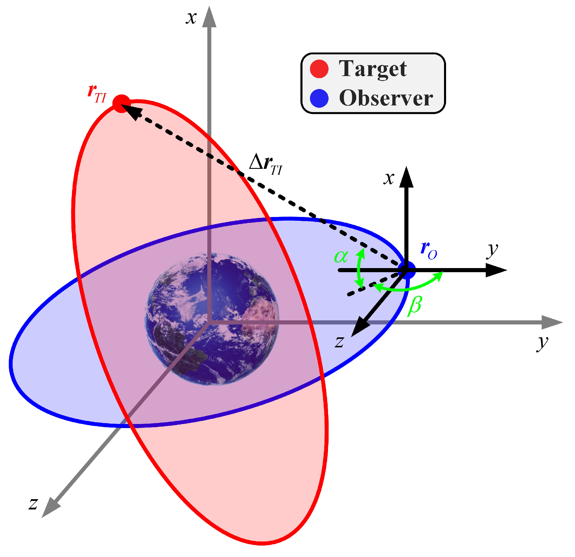
2.2. Measurement Model

As illustrated in Figure 1, the inter-spacecraft inertial LOS measurement can be represented by two angular measurements, i.e., the declination $\alpha$ and the right ascension $\beta$. The declination $\alpha$ is the angle relative to the inertial x-axis and between the inertial x-y plane. The right ascension $\beta$ is the angle between the inertial x-axis and the inter-spacecraft relative position vector $\Delta {\mathit{r}}_{Ti}={[\Delta x_{Ti},\Delta y_{Ti};\Delta z_{Ti}]}^T={\mathit{r}}_O-{\mathit{r}}_{Ti}$. The measurement equation of the i-th target is given as [5,41]:

$${\mathit{z}}_{Ti}=\mathit{h}\left({\mathit{x}}_{Ti}\right)+\mathit{\epsilon }=\left[\begin{array}{c}\alpha +{\epsilon }_{\rho }\\ \beta +{\epsilon }_{\dot{\rho }}\end{array}\right]=\left[\begin{array}{c}{tan}^{-1}\frac{\Delta z_{Ti}}{\sqrt{\Delta x_{Ti}^2+\Delta y_{Ti}^2}}+{\epsilon }_{\alpha }\\ {tan}^{-1}\frac{\Delta y_{Ti}}{\Delta x_{Ti}}+{\epsilon }_{\beta }\end{array}\right]$$

(4)

where $\mathit{\epsilon }={[{\epsilon }_{\alpha },{\epsilon }_{\beta }]}^T$ is the Gaussian-distributed measurement noise with the covariance matrix given by $\mathit{R}\in {\mathbb{R}}^{2\times 2}$.

The goal of the multi-spacecraft tracking is to estimate the states of the targets. The tracking system is given as:

$$\left\{\begin{array}{c}{\mathit{x}}_{Ti}\left(t_{k+1}\right)=\mathit{F}\left({\mathit{x}}_{Ti}\left(t_k\right),\Delta t_k\right)\hfill \\ {\mathit{z}}_{Ti}\left(t_{k+1}\right)=\mathit{h}\left({\mathit{x}}_{Ti}\left(t_{k+1}\right)\right)+\mathit{\epsilon }\hfill \end{array}\right.$$

(5)

Note that this paper aims at proposing a general method that does not rely on particular dynamic and measurement equations. The Earth-centered dynamic and inertial LOS measurement models are taken as an example for simulation, and the proposed method can be applied for other scenarios.

3. Methodology of the Multi-Spacecraft Tracking

The method proposed in this paper can be divided into three portions, i.e., the uncertainty propagation, the data association and the orbit estimation, which are detailed in Section 3.1, Section 3.2 and Section 3.3, respectively. Then, the overall procedure of the proposed approach is presented in Section 3.4.

3.1. Uncertainty Propagation

In this paper, the purpose of the uncertainty propagation is to predict the uncertainty distribution of the measurement at a future epoch, on which to base the optimal association model, is established for data association. The concept of uncertainty propagation is originally put forward for predicting the orbital uncertainty. In this paper, the concept of uncertainty propagation is extended into the measurement uncertainty prediction, and a semi-analytical prediction method is proposed based on the STT technique.

According to [34], the relationship between state deviations $\delta {\mathit{x}}_{Ti}\left(t_k\right)$ and $\delta {\mathit{x}}_{Ti}\left(t_{k+1}\right)$ can be represented by a second-order STT as follows:

$$\delta {\mathit{x}}_{Ti}^p\left(t_{k+1}\right)={\mathbf{\Phi }}_{Ti}^{p,l}\left(t_k,t_{k+1}\right)\delta {\mathit{x}}_{Ti}^l\left(t_k\right)+\frac{1}{2}{\mathbf{\Psi }}_{Ti}^{p,l_1{l}_2}\left(t_k,t_{k+1}\right)\delta {\mathit{x}}_{Ti}^{l_1}\left(t_k\right)\delta {\mathit{x}}_{Ti}^{l_2}\left(t_k\right)$$

(6)

where the superscripts ‘p’, ‘$l_1$’ and ‘$l_2$’ denote the p-th, $l_1$-th and $l_2$-th elements, respectively; ${\mathbf{\Phi }}_{Ti}\left(t_k,t_{k+1}\right)$ and ${\mathbf{\Psi }}_{Ti}\left(t_k,t_{k+1}\right)$ are the first-order and second-order STTs, given by:

$${\mathbf{\Phi }}_{Ti}^{p,l}\left(t_k,t_{k+1}\right)=\frac{\partial {\mathit{x}}_{Ti}^{{\displaystyle p}}\left(t_{k+1}\right)}{\partial {\mathit{x}}_{Ti}^l\left(t_k\right)}$$

(7)

$${\mathbf{\Psi }}_{Ti}^{p,l_1{l}_2}\left(t_k,t_{k+1}\right)=\frac{{\partial }^2{\mathit{x}}_{Ti}^p\left(t_{k+1}\right)}{\partial {\mathit{x}}_{Ti}^{l_1}\left(t_k\right)\partial {\mathit{x}}_{Ti}^{l_2}\left(t_k\right)}$$

(8)

Note that, for brevity, summation convention is used in Equation (6). As an example, for the second-order term in Equation (6), the summation convention is expressed as:

$${\mathbf{\Psi }}_{Ti}^{p,l_1{l}_2}\left(t_k,t_{k+1}\right)\delta {\mathit{x}}_{Ti}^{l_1}\left(t_k\right)\delta {\mathit{x}}_{Ti}^{l_2}\left(t_k\right)=\sum _{l_1=1}^6\sum _{l_2=1}^6{\mathbf{\Psi }}_{Ti}^{p,l_1{l}_2}\left(t_k,t_{k+1}\right)\delta {\mathit{x}}_{Ti}^{l_1}\left(t_k\right)\delta {\mathit{x}}_{Ti}^{l_2}\left(t_k\right)$$

(9)

The first-order STT ${\mathbf{\Phi }}_{Ti}\left(t_k,t_{k+1}\right)$ and the second-order STT ${\mathbf{\Psi }}_{Ti}\left(t_k,t_{k+1}\right)$ can be computed by integrating the following differential equations:

$${\dot{\mathbf{\Phi }}}_{Ti}^{p,l}\left(t_k,t\right)={\mathit{f}}_{*}^{p,\alpha }{\mathbf{\Psi }}_{Ti}^{\alpha ,l}\left(t_k,t\right)$$

(10)

$${\dot{\mathbf{\Psi }}}_{Ti}^{p,l_1{l}_2}\left(t_k,t\right)={\mathit{f}}_{*}^{p,\alpha }{\mathbf{\Psi }}_{Ti}^{\alpha ,l_l{l}_2}\left(t_k,t\right)+{\mathit{f}}_{*}^{p,\alpha \beta }{\mathbf{\Phi }}_{Ti}^{\alpha ,l_1}\left(t_k,t\right){\mathbf{\Phi }}_{Ti}^{\beta ,l_2}\left(t_k,t\right)$$

(11)

where:

$${\mathit{f}}_{*}^{p,\alpha }=\frac{\partial {\dot{\mathit{x}}}_{Ti}^p\left(t\right)}{\partial {\mathit{x}}_{Ti}^{\alpha }\left(t\right)}$$

(12)

$${\mathit{f}}_{*}^{p,\alpha \beta }=\frac{{\partial }^2{\dot{\mathit{x}}}_{Ti}^p\left(t\right)}{\partial {\mathit{x}}_{Ti}^{\alpha }\left(t\right)\partial {\mathit{x}}_{Ti}^{\beta }\left(t\right)}$$

(13)

The details on how these differential equations are obtained are well provided by Park and Scheeres [34]. For brevity, they are not given in this paper, and any reader with particular interest on this issue can refer to [34]. In this paper, for the dynamics mentioned in Equations (1) and (2), the partials in Equations (12) and (13) are analytically computed using the MATLAB’s symbolic toolbox (MATLAB version R2019a, The MathWorks, Inc., Natick, MA, USA).

Moreover, the measurement equation in Equation (4) can be approximated by a second-order expression as:

$$\delta {\mathit{z}}_{Ti}^p\left(t_k\right)={\mathbf{\Omega }}_{Ti}^{p,l}\left(t_k\right)\delta {\mathit{x}}_{Ti}^l\left(t_k\right)+\frac{1}{2}{\mathbf{\Xi }}_{Ti}^{p,l_1{l}_2}\left(t_k\right)\delta {\mathit{x}}_{Ti}^{l_1}\left(t_k\right)\delta {\mathit{x}}_{Ti}^{l_2}\left(t_k\right)$$

(14)

where ${\mathbf{\Omega }}_{Ti}\left(t_k\right)$ and ${\mathbf{\Xi }}_{Ti}\left(t_k\right)$ are the first-order and second-order coefficients of the LOS measurement equation:

$${\mathbf{\Omega }}_{Ti}^{p,l}\left(t_k\right)=\frac{\partial {\mathit{z}}_{Ti}^p\left(t_k\right)}{\partial {\mathit{x}}_{Ti}^l\left(t_k\right)}$$

(15)

$${\mathbf{\Xi }}_{Ti}^{p,l_1{l}_2}\left(t_k\right)=\frac{{\partial }^2{\mathit{z}}_{Ti}^p\left(t_k\right)}{\partial {\mathit{x}}_{Ti}^{l_1}\left(t_k\right)\partial {\mathit{x}}_{Ti}^{l_2}\left(t_k\right)}$$

(16)

Subscribe Equations (14)–(16) into Equation (6) and neglect all the terms higher than second-order. Then, a second-order semi-analytical solution for measurement prediction is proposed as:

$$\begin{array}{cc}\hfill \delta {\mathit{z}}_{Ti}^p\left(t_{k+1}\right)=& {\mathbf{\Omega }}_{Ti}^{p,l}\left(t_{k+1}\right)\left[{\mathbf{\Phi }}_{Ti}^{l,m}\left(t_k,t_{k+1}\right)\delta {\mathit{x}}_{Ti}^m\left(t_k\right)+\frac{1}{2}{\mathbf{\Psi }}_{Ti}^{l,m_1{m}_2}\left(t_k,t_{k+1}\right)\delta {\mathit{x}}_{Ti}^{m_1}\left(t_k\right)\delta {\mathit{x}}_{Ti}^{m_2}\left(t_k\right)\right]\hfill \\ \hfill & +\frac{1}{2}{\mathbf{\Xi }}_{Ti}^{p,l_1{l}_2}\left(t_{k+1}\right){\mathbf{\Phi }}_{Ti}^{l_1,m_1}\left(t_k,t_{k+1}\right)\delta {\mathit{x}}_{Ti}^{m_1}\left(t_k\right){\mathbf{\Phi }}_{Ti}^{l_2,m_2}\left(t_k,t_{k+1}\right)\delta {\mathit{x}}_{Ti}^{m_2}\left(t_k\right)\hfill \end{array}$$

(17)

The proposed second-order semi-analytical propagation can be further simplified as:

$$\delta {\mathit{z}}_{Ti}^p\left(t_{k+1}\right)={\mathit{G}}_{Ti}^{p,m}\left(t_k,t_{k+1}\right)\delta {\mathit{x}}_{Ti}^m\left(t_k\right)+\frac{1}{2}{\mathit{H}}_{Ti}^{p,m_1{m}_2}\left(t_k,t_{k+1}\right)\delta {\mathit{x}}_{Ti}^{m_1}\left(t_k\right)\delta {\mathit{x}}_{Ti}^{m_2}\left(t_k\right)$$

(18)

where ${\mathit{G}}_{Ti}\left(t_k,t_{k+1}\right)$ and ${\mathit{H}}_{Ti}\left(t_k,t_{k+1}\right)$ are the corresponding STTs for measurement prediction:

$${\mathit{G}}_{Ti}^{p,m}\left(t_k,t_{k+1}\right)={\mathbf{\Omega }}_{Ti}^{p,l}\left(t_{k+1}\right){\mathbf{\Psi }}_{Ti}^{l,m}\left(t_k,t_{k+1}\right)$$

(19)

$${\mathit{H}}_{Ti}^{p,m_1{m}_2}\left(t_k,t_{k+1}\right)={\mathbf{\Omega }}_{Ti}^{p,l}\left(t_{k+1}\right){\mathbf{\Psi }}_{Ti}^{l,m_i{m}_2}\left(t_k,t_{k+1}\right)+{\mathbf{\Xi }}_{Ti}^{p,l,l_2}\left(t_{k+1}\right){\mathbf{\Phi }}_{Ti}^{l_1,m_1}\left(t_k,t_{k+1}\right){\mathbf{\Phi }}_{Ti}^{l_2,m_2}\left(t_k,t_{k+1}\right)$$

(20)

The second-order semi-analytical propagation in Equation (18) can predict the future measurement deviation ${\mathit{z}}_{Ti}\left(t_{k+1}\right)$ based on the current orbit estimation ${\mathit{x}}_{Ti}\left(t_k\right)$. To distinguish the STTs ${\mathit{G}}_{Ti}\left(t_k,t_{k+1}\right)$ and ${\mathit{H}}_{Ti}\left(t_k,t_{k+1}\right)$ with the STTs ${\mathbf{\Phi }}_{Ti}\left(t_k,t_{k+1}\right)$ and ${\mathbf{\Psi }}_{Ti}\left(t_k,t_{k+1}\right)$, in this paper, the STTs in Equations (7) and (8) are called the state transfer STTs and the STTs in Equations (19) and (20) are called the measurement prediction STTs. Let ${\widehat{\mathit{x}}}_{Ti}\left(t_k\right)$ and ${\mathit{P}}_{Ti}\left(t_k\right)$ be the estimated state and associated covariance matrix of the i-th target at the current epoch $t_k$. According to [38], the predicted LOS measurement ${\widehat{\mathit{z}}}_{Ti}\left(t_{k+1}\right)$ and associated covariance matrix $\mathit{P}\left({\widehat{\mathit{z}}}_{Ti}\left(t_{k+1}\right)\right)$ at the future epoch $t_{k+1}$ can be obtained using the STTs in Equations (18)–(20) as:

$${\widehat{\mathit{z}}}_{Ti}^p\left(t_{k+1}\right)={\mathit{h}}^p\left(\mathit{F}\left({\widehat{\mathit{x}}}_{Ti}\left(t_k\right),\Delta t_k\right)\right)+\frac{1}{2}{\mathit{H}}_{Ti}^{p,m_1{m}_2}\left(t_k,t_{k+1}\right){\mathit{P}}_{Ti}^{m_1{m}_2}\left(t_k\right)$$

(21)

$$\begin{array}{cc}\hfill {\mathit{P}}^{p_1{p}_2}\left({\widehat{\mathit{z}}}_{Ti}\left(t_{k+1}\right)\right)=& {\mathit{G}}_{Ti}^{p_1,m_1}\left(t_k,t_{k+1}\right){\mathit{G}}_{Ti}^{p_2,m_2}\left(t_k,t_{k+1}\right){\mathit{P}}_{Ti}^{m_1{m}_2}\left(t_k\right)\hfill \\ \hfill & -\frac{1}{4}\left[{\mathit{H}}_{Ti}^{p_1,m_1{m}_2}\left(t_k,t_{k+1}\right){\mathit{P}}_{Ti}^{m_1{m}_2}\left(t_k\right)\right]\left[{\mathit{H}}_{Ti}^{p_2,m_1{m}_2}\left(t_k,t_{k+1}\right){\mathit{P}}_{Ti}^{m_1{m}_2}\left(t_k\right)\right]\hfill \\ \hfill & +\frac{1}{4}{\mathit{H}}_{Ti}^{p_1,ab}\left(t_k,t_{k+1}\right){\mathit{H}}_{Ti}^{p_2,\alpha \beta }\left(t_k,t_{k+1}\right)\left[{\mathit{P}}_{Ti}^{ab}\left(t_k\right){\mathit{P}}_{Ti}^{\alpha \beta }\left(t_k\right)+{\mathit{P}}_{Ti}^{a\alpha }\left(t_k\right){\mathit{P}}_{Ti}^{b\beta }\left(t_k\right)+{\mathit{P}}_{Ti}^{a\beta }\left(t_k\right){\mathit{P}}_{Ti}^{b\alpha }\left(t_k\right)\right]\hfill \end{array}$$

(22)

The predictions in Equations (21) and (22) are used to compare with the true measurements, and then decisions are made on whether they are matched. It can be seen from Equations (21) and (22) that the predicted LOS measurement ${\widehat{\mathit{z}}}_{Ti}\left(t_{k+1}\right)$ and associated covariance matrix $\mathit{P}\left({\widehat{\mathit{z}}}_{Ti}\left(t_{k+1}\right)\right)$ are only related to the current state of the i-th target. Thus, these predictions can be obtained in a decentralized computing framework to further reduce the computational overhead. The process of data association is detailed in the following subsection.

3.2. Data Association

The data association is to identify the conjunction between the incoming measurements and the targets. Assume that, at the epoch $t_{k+1}$, there exists N targets and M observations. Note that N can be equal to, be larger than, or be smaller than M. If $N>M$, then some targets are lost in the version. If $N<M$, then some unknown targets are added. The one-to-one correspondence between individual targets and measurements are represented by an association matrix $\mathit{\lambda }$ as:

$$\mathit{\lambda }={\left[{\lambda }_{ij}\right]}_{N\times M}\in {\mathbb{R}}^{N\times M}$$

(23)

where ${\lambda }_{ij}$ is the element at i-th row and j-th column. ${\lambda }_{ij}=1$ means the j-th observation belongs to the i-th target. Obviously, the elements should satisfy the following equations:

$$\sum _{i=1}^N{\lambda }_{ij}\le 1$$

(24)

$$\sum _{j=1}^M{\lambda }_{ij}\le 1$$

(25)

Let ${\mathit{z}}_j\left(t_{k+1}\right)$ be the j-th observation. According to Equations (21) and (22), the probability of the j-th observation being associated with the i-th target is given as:

$$p_{ij}=\frac{1}{{\left(2\pi \right)}^{q/2}∥\mathit{P}\left({\widehat{\mathit{z}}}_{T_i}\right)+\mathit{R}∥}exp\left\{-\frac{1}{2}{\left({\mathit{z}}_j-{\widehat{\mathit{z}}}_{T_i}\right)}^T{\left(\mathit{P}\left({\widehat{\mathit{z}}}_{T_i}\right)+\mathit{R}\right)}^{-1}\left({\mathit{z}}_j-{\widehat{\mathit{z}}}_{T_i}\right)\right\}$$

(26)

where $q=2$ is the dimension of the LOS measurement in Equation (4). Note that the covariance matrix $\mathit{R}$ is added in Equation (26) to compensate the errors caused by the measurement noise.

First, the targets that are not detected by the observer are identified. These targets meet the following condition:

$$\forall j\in \{1,2,\cdots ,M\},p_{ij}\le \eta$$

(27)

where $\eta$ is a user-defined threshold for target detection. In this paper, the threshold is set as $\eta ={10}^{-4}$.

Then, the optimal association problem is established as:

$$\begin{array}{cc}max\hfill & \sum _{i=1}^N\sum _{j=1}^M{\lambda }_{ij}ln\left(p_{ij}\right)\hfill \\ \mathrm{s}.\mathrm{t}.\hfill & \sum _{i=1}^N{\lambda }_{ij}\le 1\hfill \\ \hfill & \sum _{j=1}^M{\lambda }_{ij}\le 1\hfill \end{array}$$

(28)

The problem in Equation (28) is inherently a task allocation problem. A lot of approaches have been proposed to cope with the task allocation problems, which can be broadly divided into the centralized ones and decentralized ones [42,43]. The decentralized methods outperform the centralized methods in terms of the efficiency. Aiming at developing a real-time tracking framework, in this study, the contract network algorithm [43] is selected to solve the optimal association problem in Equation (28). In the researched optimal association problem, the observations ${\mathit{z}}_j\left(t_{k+1}\right)$ can be considered as tasks, and each target corresponds to one bidder. According to the contract network algorithm, the optimal association problem can be solved using four stages: the task announcement stage, the bidding stage, the awarding stage, and the monitoring stage.

In the task announcement stage, the tender information related to the data association is informed to all the potential bidders (i.e., N targets). The information includes M observations (${\mathit{z}}_j\left(t_{k+1}\right)j\in \{1,2,\cdots ,M\}$) and the covariance matrix of the measurement noise. In the bidding stage, N targets receive the tender information, and then evaluate the performance of the contract changes according to Equation (26) and their current state. In the awarding stage, the data association performance in Equation (28) will be evaluated after accepting all the bids. According to the evaluation results, the communication mechanism is multicast communication mode. The optimization process is in this stage. Finally, in the monitoring stage, the association relationship is determined. After the data association, the true measurements of each target are obtained. Then, the orbit estimation is performed using the Kalman filter.

3.3. Orbit Estimation

In this subsection, the orbit estimation is implemented using the Kalman filter. As the second-order STTs of the dynamic and measurement equations are obtained in Section 3.1, the SEKF is used for convenience. The SEKF is a special case of the high-order numerical extended Kalman filter (HNEKF). The HNEKF uses the high-order STTs to propagate the dynamic and measurement equations and has appropriate accuracy and efficiency. The detailed derivations of are provided by Park and Scheeres [34]. In this paper, the process of the SEKF is briefly given as follows.

SEKF prediction equations:

$$\delta {\widehat{\mathit{x}}}^l\left(t_{k+1};t_k\right)=\frac{1}{2}{\mathbf{\Psi }}^{l,m_1{m}_2}\left(t_k,t_{k+1}\right){\mathit{P}}^{m_1{m}_2}\left(t_k\right)$$

(29)

$${\widehat{\mathit{x}}}^l\left(t_{k+1};t_k\right)={\mathit{F}}^l\left(\widehat{\mathit{x}}\left(t_k\right),\Delta t_k\right)+\delta {\widehat{\mathit{x}}}^l\left(t_{k+1};t_k\right)$$

(30)

$$\begin{array}{cc}\hfill {\mathit{P}}^{p_1{p}_2}\left(t_{k+1};t_k\right)=& {\mathbf{\Phi }}^{p_1,m_1}\left(t_k,t_{k+1}\right){\mathbf{\Phi }}^{p_2,m_2}\left(t_k,t_{k+1}\right){\mathit{P}}^{m_1{m}_2}\left(t_k\right)-\delta {\mathit{x}}^{p_1}\left(t_{k+1};t_k\right)\delta {\mathit{x}}^{p_2}\left(t_{k+1};t_k\right)\hfill \\ \hfill & +\frac{1}{4}{\mathbf{\Psi }}^{p_1,ab}\left(t_k,t_{k+1}\right){\mathbf{\Psi }}^{p_2,\alpha \beta }\left(t_k,t_{k+1}\right)\left[{\mathit{P}}^{ab}\left(t_k\right){\mathit{P}}^{\alpha \beta }\left(t_k\right)+{\mathit{P}}^{a\alpha }\left(t_k\right){\mathit{P}}^{b\beta }\left(t_k\right)+{\mathit{P}}^{a\beta }\left(t_k\right){\mathit{P}}^{b\alpha }\left(t_k\right)\right]\hfill \end{array}$$

(31)

SEKF update equations:

$$\delta {\widehat{\mathit{z}}}^l\left(t_{k+1}\right)=\frac{1}{2}{\mathit{H}}^{l,m_1{m}_2}\left(t_k,t_{k+1}\right){\mathit{P}}^{m_1{m}_2}\left(t_k\right)$$

(32)

$${\mathit{P}}_{zz}^{p_1{p}_2}={\mathit{P}}^{p_1{p}_2}\left({\widehat{\mathit{z}}}_{Ti}\left(t_{k+1}\right)\right)+{\mathit{R}}^{p_1{p}_2}$$

(33)

$$\begin{array}{cc}\hfill {\mathit{P}}_{xz}^{p_1{p}_2}& =\frac{1}{4}{\mathbf{\Psi }}^{p_1,ab}\left(t_k,t_{k+1}\right){\mathit{H}}^{p_2,\alpha \beta }\left(t_k,t_{k+1}\right)\left[{\mathit{P}}^{ab}\left(t_k\right){\mathit{P}}^{\alpha \beta }\left(t_k\right)+{\mathit{P}}^{a\alpha }\left(t_k\right){\mathit{P}}^{b\beta }\left(t_k\right)+{\mathit{P}}^{a\beta }\left(t_k\right){\mathit{P}}^{b\alpha }\left(t_k\right)\right]\hfill \\ \hfill & -\delta {\widehat{\mathit{x}}}^{p_1}\left(t_{k+1};t_k\right)\delta {\widehat{\mathit{z}}}^{p_2}\left(t_{k+1}\right)\hfill \end{array}$$

(34)

$$\mathit{K}\left(t_{k+1}\right)={\mathit{P}}_{xz}{\left({\mathit{P}}_{zz}\right)}^{-1}$$

(35)

$$\widehat{\mathit{x}}\left(t_{k+1}\right)=\widehat{\mathit{x}}\left(t_{k+1};t_k\right)+\mathit{K}\left(t_{k+1}\right)\left(\mathit{z}\left(t_{k+1}\right)-\widehat{\mathit{z}}\left(t_{k+1}\right)\right)$$

(36)

$$\mathit{P}\left(t_{k+1}\right)=\mathit{P}\left(t_{k+1};t_k\right)-\mathit{K}\left(t_{k+1}\right){\mathit{P}}_{zz}{\left(\mathit{K}\left(t_{k+1}\right)\right)}^T$$

(37)

Note that, in Equations (29)–(37), the subscript ‘$Ti$’ is excluded because each target is assumed to be well associated with its measurements.

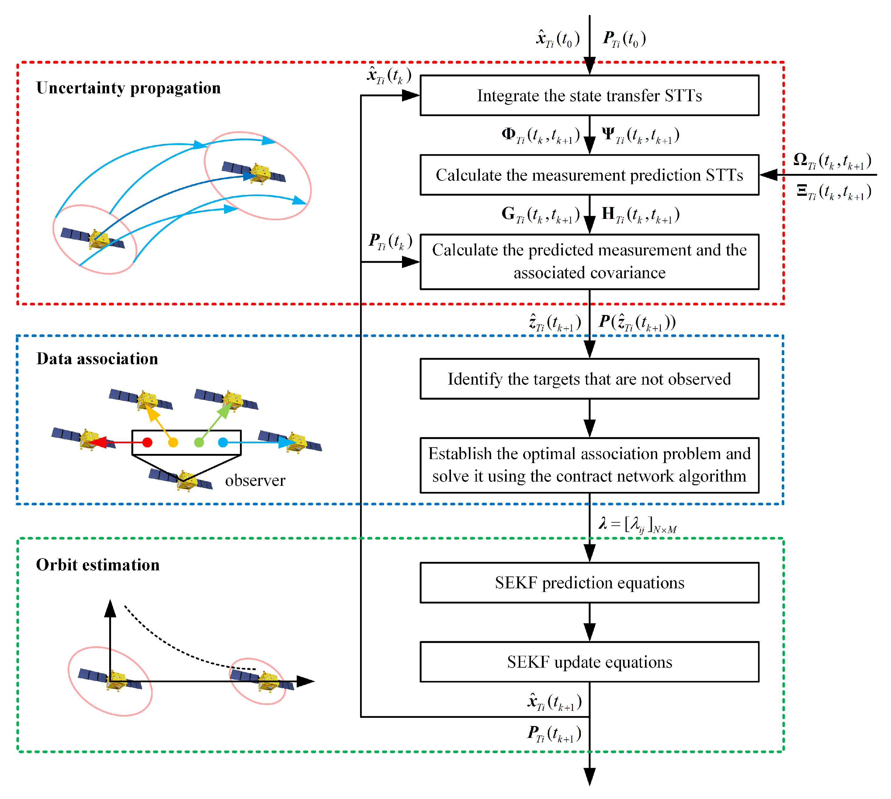
3.4. Overall Procedure

According to the descriptions in the above subsections, the overall procedure of the proposed multi-spacecraft tracking method is shown in Figure 2. In addition, the procedure steps are as follows.

Step 1: At the current epoch $t_k$, the estimated state ${\widehat{\mathit{x}}}_{Ti}\left(t_k\right)$ and the associated covariance ${\mathit{P}}_{Ti}\left(t_k\right)$ of the i-th target are available. For each target, integrate the differential equations in Equations (10)–(13) based on the estimated state ${\widehat{\mathit{x}}}_{Ti}\left(t_k\right)$, and then the state transfer STTs are obtained.

Step 2: Calculate the STTs ${\mathbf{\Omega }}_{Ti}\left(t_k\right)$ and ${\mathbf{\Xi }}_{Ti}\left(t_k\right)$ using Equations (15) and (16). Subscribe Equations (15) and (16) into Equations (19) and (20) to obtain the measurement prediction STTs. Calculate the predicted measurement ${\widehat{\mathit{z}}}_{Ti}\left(t_{k+1}\right)$ and the associated covariance matrix $\mathit{P}\left({\widehat{\mathit{z}}}_{Ti}\left(t_{k+1}\right)\right)$ based on the measurement prediction STTs.

Step 3: Identify the targets that are not observed according to Equation (27).

Step 4: Establish the optimal association problem according to Equation (28) and solve it using the contract network algorithm.

Step 5: Propagate the dynamic equations based on the obtained state transfer STTs and the SEKF.

Step 6: Update the estimated state ${\widehat{\mathit{x}}}_{Ti}\left(t_{k+1}\right)$ and the associated covariance ${\mathit{P}}_{Ti}\left(t_{k+1}\right)$ using Equations (32)–(37).

By performing the above steps, one round of tracking is finished. Let $k\leftarrow k+1$, and then the next round of tracking begins.

4. Numerical Simulation

In this section, numerical simulations are implemented to validate the performance of the proposed multi-spacecraft tracking method. A case with four targets is considered, and the accuracy of the proposed method is investigated.

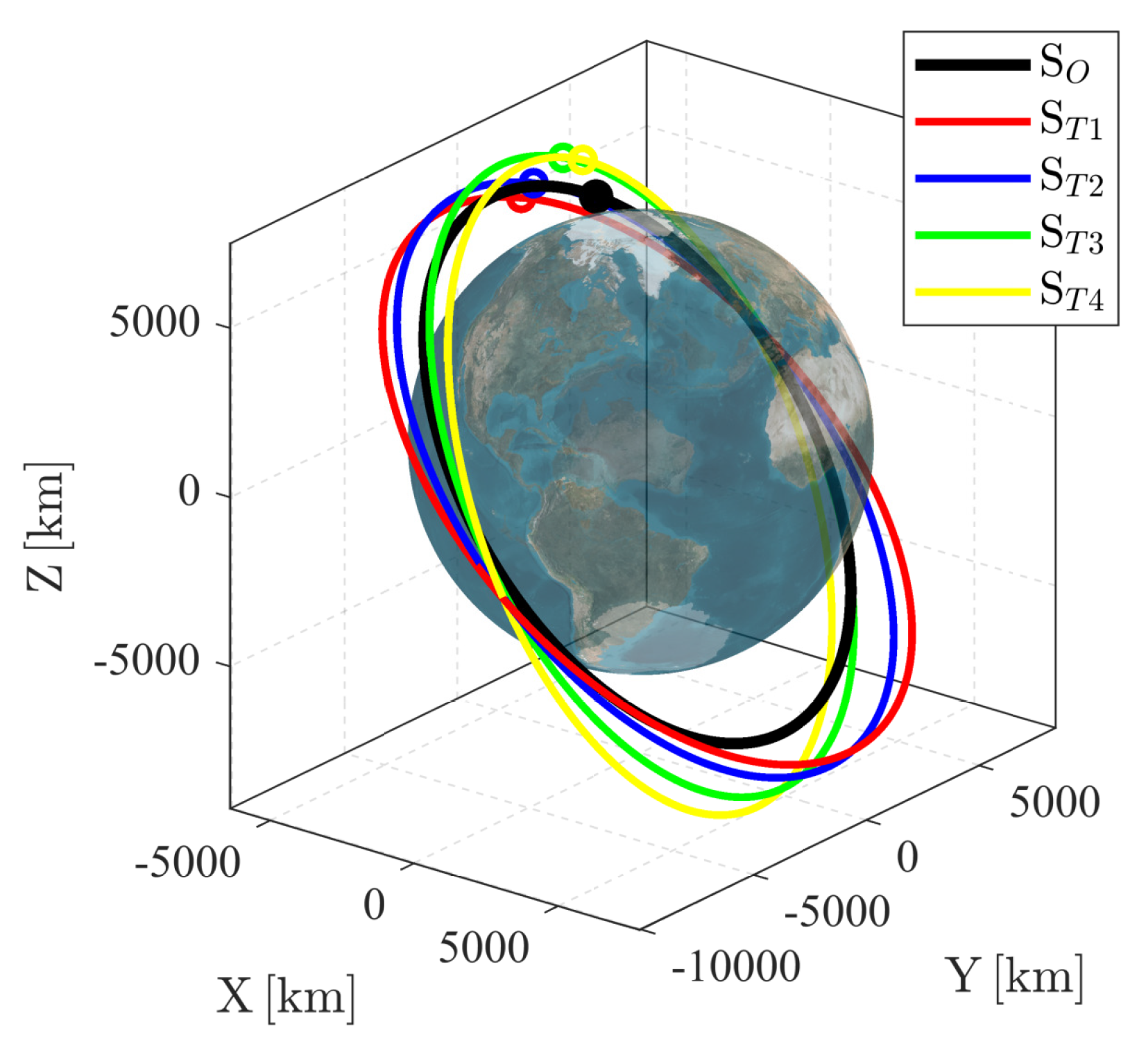
4.1. Scenario Design

The nominal orbit elements of the four targets and observer are listed in

Table 1. Nominal orbit elements of the target and the observer.

		a/km	e	i/${}^{\circ }$	$\mathbf{\Omega }$/${}^{\circ }$	$\mathit{\omega }$/${}^{\circ }$	n/${}^{\circ }$
Observer	S${}_O$	8362	0.1007	53.60	100.60	33.00	21.51
Target	S${}_{T1}$	9381	0.1498	43.60	103.1	42.00	22.02
	S${}_{T1}$	9406	0.1398	48.60	103.6	42.00	22.02
	S${}_{T2}$	9456	0.1198	58.60	104.6	42.00	22.02
	S${}_{T2}$	9481	0.1098	63.60	105.1	42.00	22.02

, where a, e, n, i, $\omega$, and $\mathsf{\Omega }$ label the semimajor axis, eccentricity, true anomaly, inclination, argument of periapsis, and longitude of the ascending node, respectively. The nominal orbits of the observer and four targets are illustrated in Figure 3. The orbit of the observer is black and the orbits of the four targets are red, blue, green, and yellow, respectively. The nominal orbit elements of the four targets are particularly designed to guarantee that their orbits cross with each other. The crossing orbits of the targets add more difficulties in the data association, in which the advantages of the proposed method can be better demonstrated.

The total tracking period is set to be 3 h, with a measurement interval of 10 s. The nominal angular measurements of the four targets are shown in Figure 4. Figure 4a illustrates the time history of the declination $\alpha$ and the right ascension $\beta$, and Figure 4b illustrates the projection of these two angular measurements. It can be seen that the orbits cross at around $t=47$ min and $t=129.5$ min.

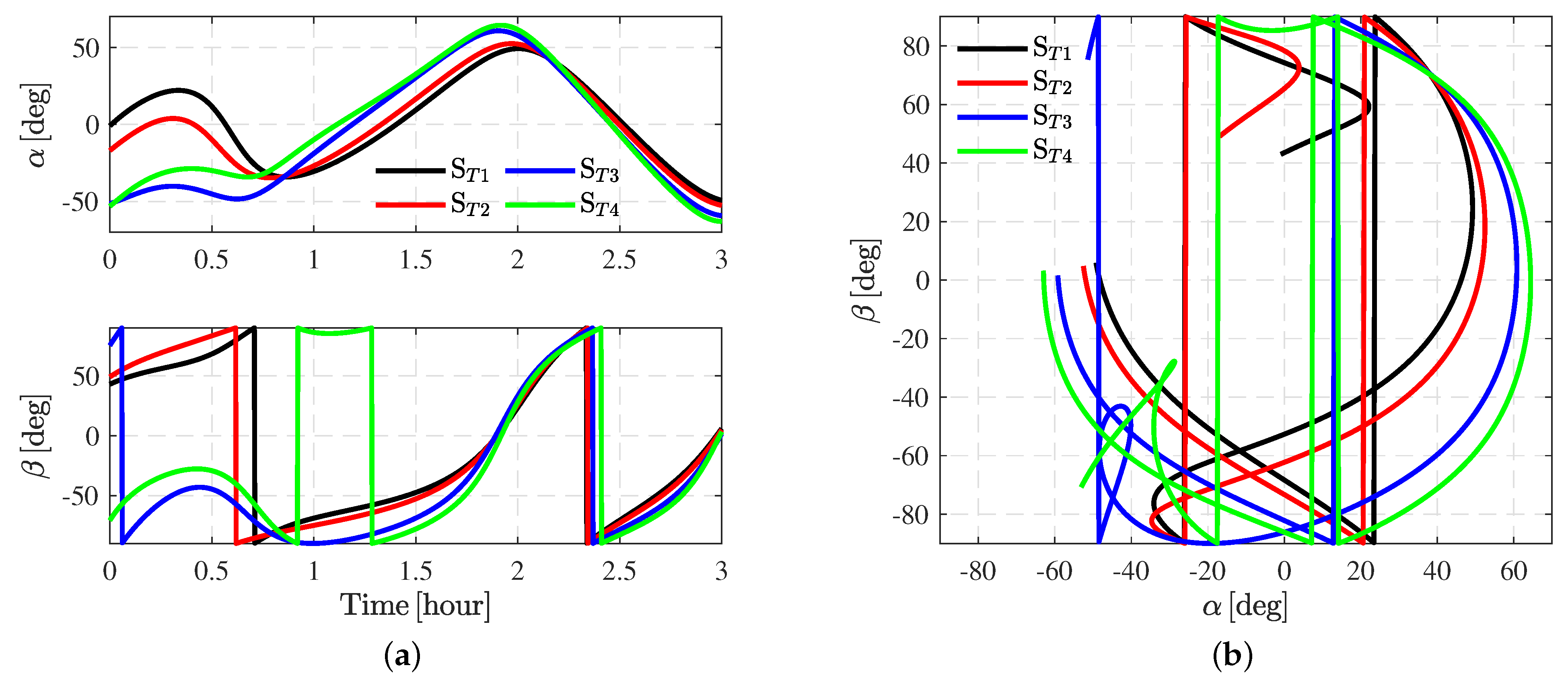
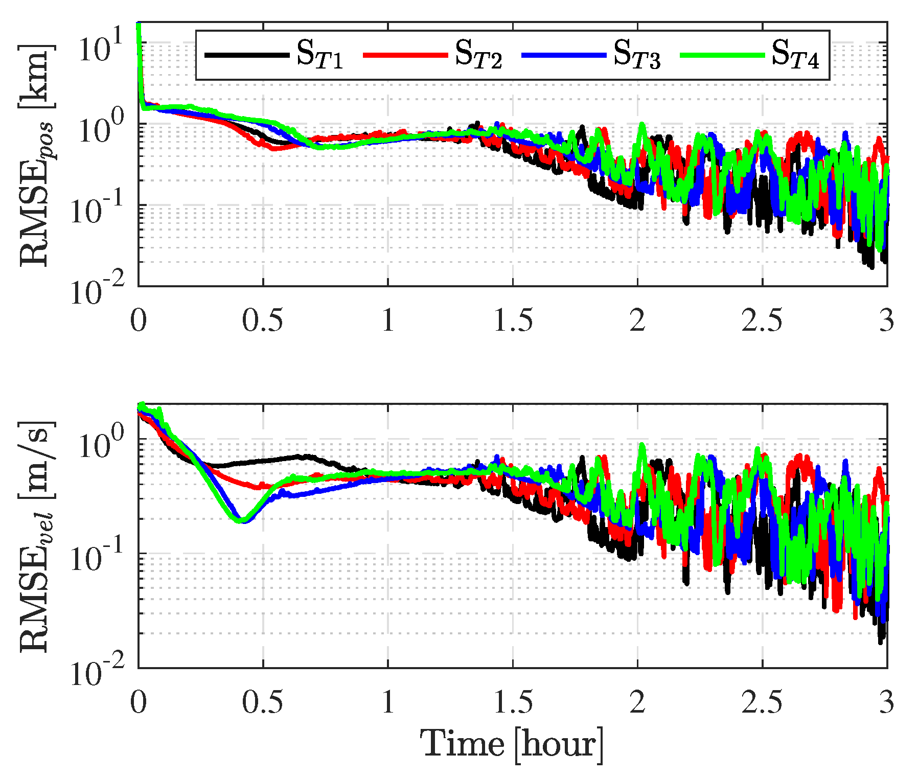
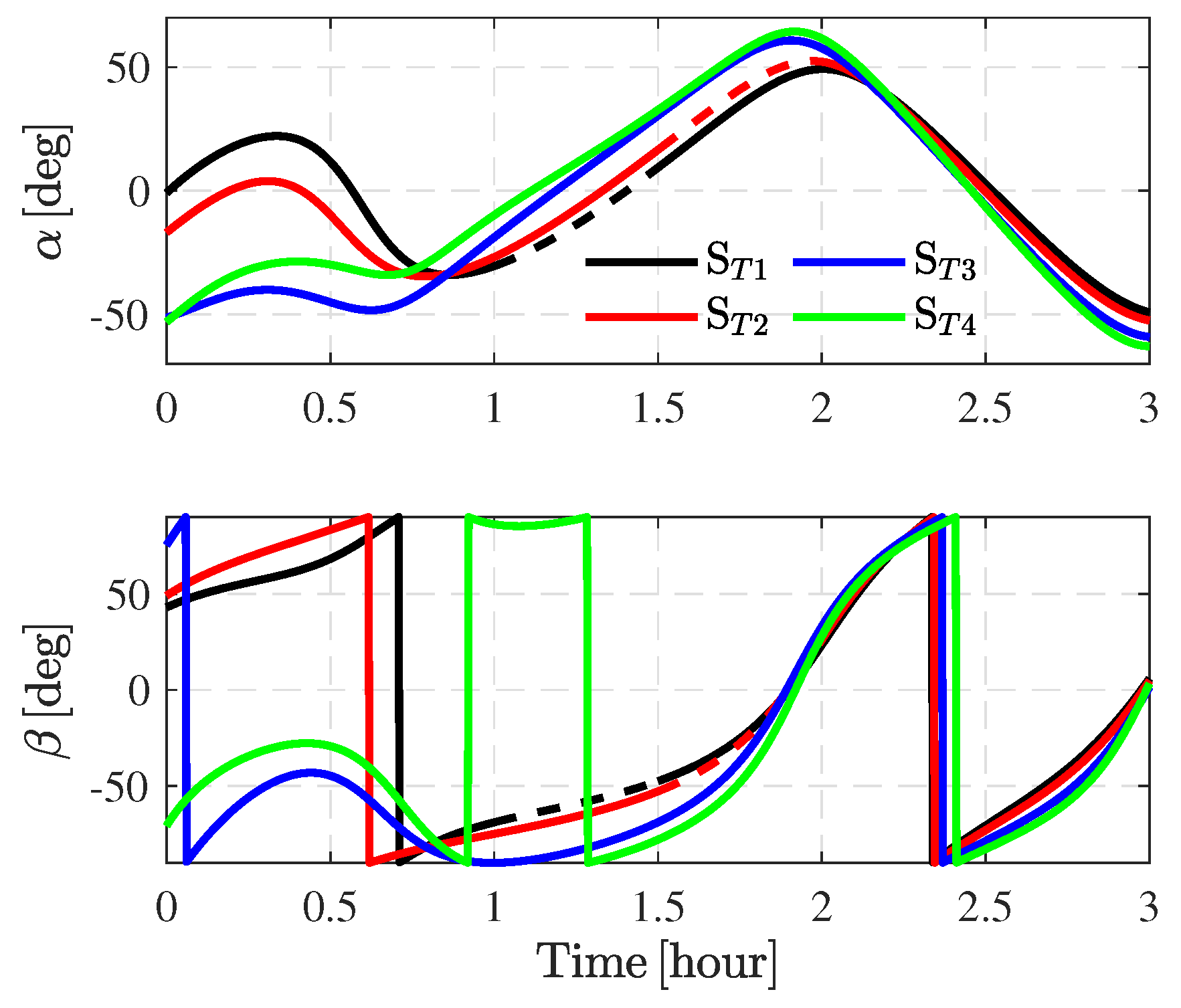
4.2. Simulation Results

First, assume that all the four targets are visible during the 3 h tracking. The initial position and velocity estimated errors are respectively set to be 10 km per axis and 1 m/s per axis. The initial covariance is given as:

$${\mathit{P}}_{Ti}\left(t_0\right)=\left[\begin{array}{cc}100{\mathit{I}}_3{\mathrm{km}}^2& {\mathbf{0}}_{3\times 3}\\ {\mathbf{0}}_{3\times 3}& 1{\mathit{I}}_3{\mathrm{m}}^2/{\mathrm{s}}^2\end{array}\right],i\in \{1,2,3,4\}$$

(38)

where ${\mathit{I}}_3$ is the three-dimensional identified matrix and ${\mathbf{0}}_{3\times 3}$ is the zero matrix.

The covariance of the measurement noise is set to be:

$$\mathit{R}=\left[\begin{array}{cc}{10}^{-4}{\mathrm{deg}}^2& {\mathbf{0}}_{3\times 3}\\ {\mathbf{0}}_{3\times 3}& {10}^{-4}{\mathrm{deg}}^2\end{array}\right]$$

(39)

The computation follows the flow chart in Figure 2.

Table 2. Data association results when $t_k=0$.

		${\mathit{z}}_1$	${\mathit{z}}_2$	${\mathit{z}}_3$	${\mathit{z}}_4$
		[−0.5569, 43.1841]	[−16.6373, 49.4247]	[−51.2908, 76.0587]	[−52.8157, −70.0077]
${\widehat{\mathit{z}}}_{T1}$	[−0.8393, 43.1550]	0.6922	$\approx 0$	$\approx 0$	$\approx 0$
${\widehat{\mathit{z}}}_{T2}$	[−17.0700, 49.4502]	$\approx 0$	0.4117	$\approx 0$	$\approx 0$
${\widehat{\mathit{z}}}_{T3}$	[−51.7809, 76.4379]	$\approx 0$	$\approx 0$	0.1785	$\approx 0$
${\widehat{\mathit{z}}}_{T4}$	[−53.1513, −69.3724]	$\approx 0$	$\approx 0$	$\approx 0$	0.1933

and

Table 3. Data association results when $t_k=129.5$ min.

		${\mathit{z}}_1$	${\mathit{z}}_2$	${\mathit{z}}_3$	${\mathit{z}}_4$
		[42.3691, 61.2692]	[42.2580, 63.1710]	[41.5619, 66.5737]	[44.3305, 64.0263]
${\widehat{\mathit{z}}}_{T1}$	[42.3522, 61.2866]	0.8767	0.1544	$7.7160\times {10}^{-7}$	0.0032
${\widehat{\mathit{z}}}_{T2}$	[42.2656, 63.1609]	0.1499	0.8682	0.0022	0.0721
${\widehat{\mathit{z}}}_{T3}$	[41.5623, 66.5585]	$6.3340\times {10}^{-7}$	0.0023	0.8544	0.0008
${\widehat{\mathit{z}}}_{T4}$	[44.3387, 64.0293]	0.0029	0.0709	0.0008	0.8576

illustrate the data association results when $t_k=0$ and $t_k=129.5$ min, respectively. $t_k=0$ denote the initial epoch and $t_k=129.5$ min is the epoch when the orbits of the four targets cross with each other. In Table 2, $\approx 0$ means that the value is smaller than ${10}^{-18}$. The real observations and the targets are well matched. Take the epoch $t_k=129.5$ min as an example. When the association matrix $\mathit{\lambda }$ is given as

$$\mathit{\lambda }=\left[\begin{array}{cccc}1\hfill & 0\hfill & 0\hfill & 0\hfill \\ 0\hfill & 1\hfill & 0\hfill & 0\hfill \\ 0\hfill & 0\hfill & 1\hfill & 0\hfill \\ 0\hfill & 0\hfill & 0\hfill & 1\hfill \end{array}\right],$$

(40)

the objective function has the largest value, i.e., ${\sum }_{i=1}^N{\sum }_{j=1}^M{\lambda }_{ij}ln\left(p_{ij}\right)=-0.5839$.

All the measurements are associated correctly. The estimated errors are shown in Figure 5, where $\mathit{e}$ and $\dot{\mathit{e}}$ represent the position and velocity estimated error:

$$\mathit{e}={\widehat{\mathit{r}}}_{Ti}-{\mathit{r}}_{Ti}$$

(41)

$$\dot{\mathit{e}}={\widehat{\mathit{v}}}_{Ti}-{\mathit{v}}_{Ti}$$

(42)

It can be seen from Figure 5 that the estimated errors converge at the epoch around 1.5 h. The converged position and velocity estimated errors are around 0.1 km and 0.1 m/s.

To further investigate the performance of the proposed method, 300 Monte Carlo runs are performed. For each target, the initial estimation ${\widehat{\mathit{x}}}_{Ti}\left(t_0\right)$ is randomly generated from the normal distribution $N({\widehat{\mathit{x}}}_{Ti}\left(t_0\right);{\mathit{x}}_{Ti}\left(t_0\right),{{\displaystyle \mathit{P}}}_{Ti}\left(t_0\right))$, in which ${\mathit{x}}_{Ti}\left(t_0\right)$ is the true initial value listed in Table 1 and ${\mathit{P}}_{Ti}\left(t_0\right)$ is the initial covariance.

All the 324,000 data associations (each Monte Carlo run contains 1080 data associations), only two measurements are incorrectly associated. The data association accuracy is 99.99%. The root mean square error (RMSE) is taken as the metrics to evaluate the performance of the proposed method. The position and velocity RMSEs are expressed as follows:

$${RMSE}_{pos}\left(t_k\right)=\sqrt{\frac{1}{100}\sum _{p=1}^{100}∥{\widehat{\mathit{r}}}_{Ti,p}\left(t_k\right)-{\mathit{r}}_{Ti,p}\left(t_k\right)∥}$$

(43)

$${RMSE}_{vel}\left(t_k\right)=\sqrt{\frac{1}{100}\sum _{p=1}^{100}∥{\widehat{\mathit{v}}}_{Ti,p}\left(t_k\right)-{\mathit{v}}_{Ti,p}\left(t_k\right)∥}$$

(44)

where $\{{\widehat{\mathit{r}}}_{Ti,p}\left(t_k\right),{\widehat{\mathit{v}}}_{Ti,p}\left(t_k\right)\}$ and $\{{\mathit{r}}_{Ti,p}\left(t_k\right),{\mathit{v}}_{Ti,p}\left(t_k\right)\}$ are the estimations and true values at the p-th Monte Carlo run.

The RMSEs of the 300 Monte Carlo runs are shown in Figure 6, and the mean RMSE is listed in

Table 4. Mean RMSE of the Monte Carlo simulation.

	S${}_{\mathit{T}1}$	S${}_{\mathit{T}2}$	S${}_{\mathit{T}3}$	S${}_{\mathit{T}4}$
Position/km	0.6181	0.6108	0.7004	0.7072
Velocity/(m/s)	0.4487	0.4197	0.4594	0.4514

. As shown in Table 4, the position and velocity RMSEs are smaller than 0.71 km and 0.46 m/s. All the four targets are well tracked. The second target (${\mathrm{S}}_{T2}$) has the best estimation accuracy, with the position and velocity RMSEs being 0.6108 km and 0.4197 m/s. The third target (${\mathrm{S}}_{T3}$) has the poorest estimation precision, with the position and velocity RMSEs being 0.7004 km and 0.4594 m/s. The differences in estimation accuracy are related to the observation configuration, which is not discussed in this paper. The readers with the interest on this issue can refer to [4,44,45,46].

The simulations are performed using MATLAB R2018b on a computer with a 3.6 GHz AMD Ryzen processer and a 16 GB RAM. The mean one-step run time of the proposed method is 25.2532 ms, which means that the proposed method is efficient and can be used for real-time tracking.

Then, the case considering invisible targets are investigated. Assume that the first target (${\mathrm{S}}_{T1}$) is invisible from the epoch $t=1$ h to the epoch $t=1.5$ h and the second target (${\mathrm{S}}_{T2}$) is invisible from the epoch $t=1.5$ h to the epoch $t=2$ h. The measurements are shown in Figure 7. In Figure 7, the visible and invisible arcs are represented by the solid lines and the dashed lines, respectively.

The RMSEs of ${\mathrm{S}}_{T1}$ and ${\mathrm{S}}_{T2}$ are shown in Figure 8 and

Table 5. Mean RMSE of the Monte Carlo simulation considering invisible arcs.

	S${}_{\mathit{T}1}$	S${}_{\mathit{T}2}$
Position/km	0.6147	0.6169
Velocity/(m/s)	0.4309	0.4078

. The RMSEs of ${\mathrm{S}}_{T3}$ and ${\mathrm{S}}_{T4}$ are not shown as they are always visible during tracking, and the results are very close to that in Figure 6 and Table 4. It can be seen that the two targets are accurately tracked during the visible arcs. The position and velocity RMSEs are around 0.61 km and 0.43 m/s, which are a little larger than the visible case.

5. Conclusions

This paper proposed a multi-spacecraft tracking and data association method based on the uncertainty propagation. A series of second-order analytical solutions are proposed for accurate measurement prediction. Based on the proposed second-order analytical solutions, the optimal data association problem is established and then solved in a distributed framework. Finally, a second-order extended Kalman filter is designed after the observations and the targets are matched. The proposed method is successfully applied into solving an angle-only four-spacecraft tracking problem. The simulated scenario is specifically designed to increase the difficulty of the date association, with the orbits of the four targets crossing with each other. Simulations show that all the targets are well tracked. The data association accuracy of the proposed method is higher than 99.99%, meaning that the proposed second-order analytical solution is accurate enough to predict the measurement. The mean one-step run time is only 25.25 ms. The position and velocity estimated errors are around 0.6 km and 0.4 m/s when the standard deviation of the measurements is 0.01°. Furthermore, as the proposed second-order analytical solution can provide precise prediction, the targets are correctly identified and the orbits are accurately estimated even after the one-hour invisible arcs. In the future, the multi-spacecraft tracking problem considering an unknown maneuver can be further studied. Moreover, the initial orbit determination method for the multi-spacecraft scenario can be investigated.

References

1. Lee, S.; Lee, J.; Hwang, I. Maneuvering spacecraft tracking via state-dependent adaptive estimation. J. Guid. Control Dyn. 2016, 39, 2034–2043. [Google Scholar] [CrossRef]
2. Ko, H.C.; Scheeres, D.J. Tracking maneuvering satellite using thrust-fourier-coefficient event representation. J. Guid. Control Dyn. 2016, 39, 216–221. [Google Scholar] [CrossRef]
3. Serra, R.; Yanez, C.; Frueh, C. Tracklet-to-orbit association for maneuvering space objects using optimal control theory. Acta Astronaut. 2021, 181, 271–281. [Google Scholar] [CrossRef]
4. Luo, Y.; Qin, T.; Zhou, X. Observability Analysis and Improvement Approach for Cooperative Optical Orbit Determination. Aerospace 2022, 9, 166. [Google Scholar] [CrossRef]
5. Qiao, D.; Zhou, X.; Zhao, Z.; Qin, T. Asteroid Approaching Orbit Optimization Considering Optical Navigation Observability. IEEE Trans. Aerosp. Electron. Syst. 2022. [Google Scholar] [CrossRef]
6. Zhou, X.; Qin, T.; Meng, L. Maneuvering Spacecraft Orbit Determination Using Polynomial Representation. Aerospace 2022, 9, 257. [Google Scholar] [CrossRef]
7. Tang, Y.; Wu, W.; Qiao, D.; Li, X. Effect of orbital shadow at an Earth-Moon Lagrange point on relay communication mission. Sci. China Inf. Sci. 2017, 60, 1–10. [Google Scholar] [CrossRef] [Green Version]
8. Wu, W.; Tang, Y.; Zhang, L.; Qiao, D. Design of communication relay mission for supporting lunar-farside soft landing. Sci. China Inf. Sci. 2018, 61, 040305. [Google Scholar] [CrossRef]
9. Li, X.; Qiao, D.; Barucci, M.A. Analysis of equilibria in the doubly synchronous binary asteroid systems concerned with non-spherical shape. Astrodynamics 2018, 2, 133–146. [Google Scholar] [CrossRef]
10. Li, X.; Qiao, D.; Li, P. Frozen orbit design and maintenance with an application to small body exploration. Aerosp. Sci. Technol. 2019, 92, 170–180. [Google Scholar] [CrossRef]
11. Colagrossi, A.; Lavagna, M. Fault Tolerant Attitude and Orbit Determination System for Small Satellite Platforms. Aerospace 2022, 9, 46. [Google Scholar] [CrossRef]
12. Li, L.-Q.; Xie, W.-X. Intuitionistic fuzzy joint probabilistic data association filter and its application to multitarget tracking. Signal Process. 2014, 96, 433–444. [Google Scholar] [CrossRef]
13. Wen, H.; Fan, H.; Xie, W.; Pei, J. Hybrid Structure-Adaptive RBF-ELM Network Classifier. IEEE Access 2017, 5, 16539–16554. [Google Scholar] [CrossRef]
14. Oussalah, M.; De Schutter, J. Hybrid fuzzy probabilistic data association filter and joint probabilistic data association filter. Inf. Sci. 2002, 142, 195–226. [Google Scholar] [CrossRef]
15. Aziz, A.M. A new nearest-neighbor association approach based on fuzzy clustering. Aerosp. Sci. Technol. 2013, 26, 87–97. [Google Scholar] [CrossRef]
16. Sutharsan, S.; Kirubarajan, T.; Lang, T.; Mcdonald, M. An Optimization-Based Parallel Particle Filter for Multitarget Tracking. IEEE Trans. Aerosp. Electron. Syst. 2012, 48, 1601–1618. [Google Scholar] [CrossRef] [Green Version]
17. Habtemariam, B.; Tharmarasa, R.; Thayaparan, T.; Mallick, M.; Kirubarajan, T. A Multiple-Detection Joint Probabilistic Data Association Filter. IEEE J. Sel. Top. Signal Process. 2013, 7, 461–471. [Google Scholar] [CrossRef]
18. Sathyan, T.; Chin, T.J.; Arulampalam, S.; Suter, D. A Multiple Hypothesis Tracker for Multitarget Tracking With Multiple Simultaneous Measurements. IEEE J. Sel. Top. Signal Process. 2013, 7, 448–460. [Google Scholar] [CrossRef]
19. Bezdek, J.C. Pattern Recognition with Fuzzy Objective Function Algorithms; Springer Science & Business Media: Berlin/Heidelberg, Germany, 2013. [Google Scholar]
20. Fortmann, T.; Bar-Shalom, Y.; Scheffe, M. Sonar tracking of multiple targets using joint probabilistic data association. IEEE J. Ocean. Eng. 1983, 8, 173–184. [Google Scholar] [CrossRef] [Green Version]
21. Svensson, L.; Svensson, D.; Guerriero, M.; Willett, P. Set JPDA Filter for Multitarget Tracking. IEEE Trans. Signal Process. 2011, 59, 4677–4691. [Google Scholar] [CrossRef] [Green Version]
22. Rong Li, X.; Bar-Shalom, Y. Tracking in clutter with nearest neighbor filters: Analysis and performance. IEEE Trans. Aerosp. Electron. Syst. 1996, 32, 995–1010. [Google Scholar] [CrossRef]
23. Chen, X.; Tharmarasa, R.; Pelletier, M.; Kirubarajan, T. Integrated Bayesian Clutter Estimation with JIPDA/MHT Trackers. IEEE Trans. Aerosp. Electron. Syst. 2013, 49, 395–414. [Google Scholar] [CrossRef]
24. Li, X.; Qiao, D.; Chen, H. Interplanetary transfer optimization using cost function with variable coefficients. Astrodynamics 2019, 3, 173–188. [Google Scholar] [CrossRef]
25. Li, X.; Qiao, D.; Jia, F. Investigation of Stable Regions of Spacecraft Motion in Binary Asteroid Systems by Terminal Condition Maps. J. Astronaut. Sci. 2021, 68, 891–915. [Google Scholar] [CrossRef]
26. Cui, P.Y.; Qiao, D.; Cui, H.T.; Luan, E.J. Target selection and transfer trajectories design for exploring asteroid mission. Sci. China Technol. Sci. 2010, 53, 1150–1158. [Google Scholar] [CrossRef]
27. Wang, Y.; Zhang, Y.; Qiao, D.; Mao, Q.; Jiang, J. Transfer to near-Earth asteroids from a lunar orbit via Earth flyby and direct escaping trajectories. Acta Astronaut. 2017, 133, 177–184. [Google Scholar] [CrossRef]
28. Wang, Y.; Qiao, D.; Cui, P. Design of optimal impulse transfers from the Sun-Earth libration point to asteroid. Adv. Space Res. 2015, 56, 176–186. [Google Scholar] [CrossRef]
29. Jia, F.; Li, X.; Huo, Z.; Qiao, D. Mission Design of an Aperture-Synthetic Interferometer System for Space-Based Exoplanet Exploration. Space Sci. Technol. 2022, 2022, 9835234. [Google Scholar] [CrossRef]
30. Terejanu, G.; Singla, P.; Singh, T.; Scott, P.D. Adaptive Gaussian Sum Filter for Nonlinear Bayesian Estimation. IEEE Trans. Autom. Control 2011, 56, 2151–2156. [Google Scholar] [CrossRef]
31. Gelb, A.; Warren, R.S. Direct statistical analysis of nonlinear systems: CADET. AIAA J. 1973, 11, 689–694. [Google Scholar] [CrossRef]
32. Deng, Y.; Wang, Z.; Liu, L. Unscented Kalman filter for spacecraft pose estimation using twistors. J. Guid. Control Dyn. 2016, 39, 1844–1856. [Google Scholar] [CrossRef]
33. Jia, B.; Xin, M. Active Sampling Based Polynomial-Chaos–Kriging Model for Orbital Uncertainty Propagation. J. Guid. Control Dyn. 2021, 44, 905–922. [Google Scholar] [CrossRef]
34. Park, R.S.; Scheeres, D.J. Nonlinear semi-analytic methods for trajectory estimation. J. Guid. Control Dyn. 2007, 30, 1668–1676. [Google Scholar] [CrossRef] [Green Version]
35. Roa, J.; Park, R.S. Reduced nonlinear model for orbit uncertainty propagation and estimation. J. Guid. Control Dyn. 2021, 44, 1578–1592. [Google Scholar] [CrossRef]
36. Boone, S.; McMahon, J. Orbital guidance using higher-order state transition tensors. J. Guid. Control Dyn. 2021, 44, 493–504. [Google Scholar] [CrossRef]
37. Fritsch, G.S.; Demars, K.J. Nonlinear gaussian mixture filtering with intrinsic fault resistance. J. Guid. Control Dyn. 2021, 44, 2172–2185. [Google Scholar] [CrossRef]
38. Yang, Z.; Luo, Y.Z.; Lappas, V.; Tsourdos, A. Nonlinear analytical uncertainty propagation for relative motion near J2-perturbed elliptic orbits. J. Guid. Control Dyn. 2018, 41, 888–903. [Google Scholar] [CrossRef] [Green Version]
39. Yang, Z.; Luo, Y.Z.; Zhang, J. Nonlinear semi-analytical uncertainty propagation of trajectory under impulsive maneuvers. Astrodynamics 2019, 3, 61–77. [Google Scholar] [CrossRef]
40. Zhou, X.; Cheng, Y.; Qiao, D.; Huo, Z. An adaptive surrogate model-based fast planning for swarm safe migration along halo orbit. Acta Astronaut. 2022, 194, 309–322. [Google Scholar] [CrossRef]
41. Wang, Z.; Li, Z.; Wang, N.; Hoque, M.; Wang, L.; Li, R.; Zhang, Y.; Yuan, H. Real-Time Precise Orbit Determination for LEO between Kinematic and Reduced-Dynamic with Ambiguity Resolution. Aerospace 2022, 9, 25. [Google Scholar] [CrossRef]
42. De Weck, O.L.; Scialom, U.; Siddiqi, A. Optimal reconfiguration of satellite constellations with the auction algorithm. Acta Astronaut. 2008, 62, 112–130. [Google Scholar] [CrossRef]
43. Zhen, Z.; Wen, L.; Wang, B.; Hu, Z.; Zhang, D. Improved contract network protocol algorithm based cooperative target allocation of heterogeneous UAV swarm. Aerosp. Sci. Technol. 2021, 119, 107054. [Google Scholar] [CrossRef]
44. Qin, T.; Qiao, D.; Macdonald, M. Relative orbit determination using only intersatellite range measurements. J. Guid. Control Dyn. 2019, 42, 703–710. [Google Scholar] [CrossRef]
45. Qin, T.; Qiao, D.; Macdonald, M. Relative orbit determination for unconnected spacecraft within a constellation. J. Guid. Control Dyn. 2021, 44, 614–621. [Google Scholar] [CrossRef]
46. Qin, T.; Macdonald, M.; Qiao, D. Fully Decentralized Cooperative Navigation for Spacecraft Constellations. IEEE Trans. Aerosp. Electron. Syst. 2021, 57, 2383–2394. [Google Scholar] [CrossRef]
Figure 1. An illustration of the LOS-based tracking framework.
Applsci 12 07660 g001
Figure 2. Flow chart of the proposed multi-spacecraft tracking method.
Applsci 12 07660 g002
Figure 3. Illustration of the nominal orbits of the observer and targets.
Applsci 12 07660 g003
Figure 4. The nominal angular measurements. (a) time history of the two angular measurements; (b) projection of the two angular measurements.
Applsci 12 07660 g004
Figure 5. Time history of the estimated errors.
Applsci 12 07660 g005
Figure 6. Time history of the RMSEs.
Applsci 12 07660 g006
Figure 7. Time history of the two angular measurements considering invisible arcs.
Applsci 12 07660 g007
Figure 8. Time history of the RMSEs considering invisible arcs.
Applsci 12 07660 g008