Comparison of Principal-Component-Analysis-Based Extreme Learning Machine Models for Boiler Output Forecasting

Abstract

In this paper, a combined approach of Principal Component Analysis (PCA)-based Extreme Learning Machine (ELM) for boiler output forecasting in a thermal power plant is presented. The input used for this prediction model is taken from the boiler unit of the Yermarus Thermal Power Station (YTPS), India. Calculation of the accurate electrical output of a boiler in an operating system requires the knowledge of hundreds of operating parameters. The dimensionality of the input dataset is reduced by applying principal component analysis using IBM@SPSS Software. In the process of principal component analysis, a dataset of 232 parameters is standardized into 16 principal components. The total dataset collected is divided into training and testing datasets. The extreme learning machine is designed for various activation functions and the number of neurons. Sigmoid and hyperbolic tangent activation functions are studied here. Its generalization performance is examined in terms of the Mean Square Error (MSE), Mean Absolute Error (MAE), Root Mean Square (RMSE), and Mean Absolute Percentage Error (MAPE). ELM and PCA–ELM are compared. In both the ELM and PCA–ELM models, when the extreme learning machine was designed with a sigmoid activation function with 100 nodes in the hidden layer, RMSE was 5.026 and 4.730, respectively. Therefore, the developed combined approach of PCA–ELM proved as a promising technique in forecasting with reduced errors and reduced time.

1. Introduction

The growing decentralization and digitization of the power industry is driving the relevance of artificial intelligence and data analysis in particular. Today’s data science studies include a wide range of topics along the value chain, from generation and trade through transmission, distribution, and consumption. Diverse applications and different methodologies, such as various types of artificial neural networks, have also been studied. From the applications of data analysis, it can be used in four ways:

• Forecasting and Prediction.
• Monitoring and Controlling.
• Clustering.
• Others [1].

Any industrial growth story includes the thermal power industry. However, it now functions in a complicated context characterized by significant unpredictability in operational circumstances such as grid changes, a competitive market (alternative sources), fuel input, regulatory constraints, and changing staff. This creates a difficult operating environment and reduces plant profitability. Bhangu [2] proposed that with a greater rate of growth, more maintenance is required, and a complete availability analysis will aid in identifying components that are primarily responsible for low availability. It can be useful in the installation of future power plants. It is critical for the efficient and economic operation of a power plant to properly anticipate the full load electrical power output of a base load power plant. It is useful for getting the most money out of the available resources. In contrast to earlier research publications that explored data analytics in power plants and their components, Tüfekci [3] made a comparison study on multiple machine learning (ML) algorithms for predicting combined cycle power plant (CCPP) full load electrical power outputs. The prediction was done for the same using the Genetic Algorithm by Lorencin [4]. When the supplied findings were examined, artificial neural networks have much greater Root Mean Squared Error (RMSE) than other approaches, including basic regression functions. For a proper system analysis utilizing thermodynamical approaches, a significant number of assumptions are necessary, such that these assumptions account for the unpredictability of the outcome. Without these assumptions, a thermo-dynamical analysis of a real-world application would demand hundreds of nonlinear equations, the solution to which would either be impossible or would take too much time and effort. So, Kesgin [5] highlighted that machine learning algorithms are increasingly being used as an alternative to thermo-dynamical approaches to analyze systems with unpredictable input and output patterns to overcome this barrier. As a result, when considering a machine learning approach for predicting output in a power plant, various algorithms or methods can be used, but selecting the most efficient and appropriate method is critical. In [6], a hybrid Machine Learning algorithm for the prediction of landslide displacement was proposed. It was implemented for Shuping and Baishuihe landslides to calculate the hyperparameters. Ref. [7] demonstrates a support Vector Machine for the prediction of seepage-driven landslides.

As power plant equipment is complicated and difficult to predict precisely, Yuliang Dong [8] proposed an artificial neural network for condition prediction that was developed using principal component analysis (PCA). Author Wang Feiin [9] demonstrated a viable prediction model of power for grid-connected solar plants based on artificial neural networks. This neural model gives the hourly prediction value of power in steps, using the input vector as well as the past power value and other impact elements. In [10], R Mei proposed a new network model which consists of Elman Neural Networks (ENN) and principal component analysis (PCA). This prediction model helped to improve the wind power usage while also developing the stability and safety of the plant. A two-stage neural network using an Elman recurrent neural network and BP neural network was developed by L. Ma [11] to predict typical values of fault feature variables and fault types. To anticipate short-term wind power, Gang Chen [12] developed a prediction model based on a convolutional neural network (CNN) and genetic algorithm (GA) wind power prediction model for the development of wind power generation and the research status of wind power prediction technology.

Different prediction methods such as logistic regression, rule-based method, simple Bayesian classifier, artificial neural network method, k-nearest neighbor method [13], decision tree, support vector machine [14], and extreme learning machine (ELM) [15,16,17,18] can be used.

Zhou [15] found out that for small- to medium-sized training data, the user can select to utilize a method based on the training data’s size (complexity of calculation is dependent on the amount of training data) or hidden nodes’ size (complexity of computation is based on the number of hidden nodes). The dimensionality of the mapped space is determined by the number of hidden nodes. In general, the more sophisticated the training examples are, the more hidden nodes are needed to train a generalized model to estimate the target functions for a large data issue. When dealing with highly big and complicated training datasets, this causes challenges for ELM. Huang [16] found that due to the enormous number of hidden nodes required, the ELM network is quite massive, and the computing process becomes very expensive.

Huang [17] discussed the ELM method, which can be utilized to directly train neural networks using threshold functions. Many academics have lately researched extreme learning machines (ELM) as a sort of generalized single-hidden-layer feed-forward network in theory and applications. ELM’s hidden node parameters (input weights and hidden layer biases) are generated at random, and the output weights are then computed analytically using the generalized inverse approach. An ELM-based equality-constrained optimization approach with two solutions for different training data sizes was illustrated.

However, out of all these methods, Tan [19] proposed ELM. It is more efficient as ELM has a swift learning rate. ELM was applied to find out the correlation between operational parameters and nitrogen oxide emissions of the boiler. Results illustrated that the ELM model was shown to be more exact and quicker than the common artificial neural network and support vector regression models in modeling nitrogen oxide emissions.

In [20], the power flow, active power, and reactive power models of electric springs to regulate voltage were replaced by three data-driven models based on the extreme learning machine (ELM). To develop the final control strategies, an ELM-based control model was provided. In [21], an extreme learning machine (ELM) artificial neural network and four eddy current sensors were used to develop a measuring technique for the rotation angle of the spherical joint. The developed prototype showed measurement accuracy as well as offered a high-precision measuring approach. Through the determination of the picture coordinates of ripe fruits and fruit trees, the extreme learning machine algorithm was incorporated into the agricultural equipment navigation system, together with the BP neural network algorithm in [22], to accomplish the speedy navigation of the operation of agricultural machinery. The test findings reveal that employing the extreme learning machine, which can match the design criteria of contemporary agricultural machinery and equipment, has enhanced picking efficiency and accuracy significantly.

The authors addressed accurate Maximum Power Point Tracking (MPPT) for PV-based Distributed Generation (DG) in [23] using an error-optimized (via Improved Water Cycle) Extreme Learning Machine with Ridge Regression (IWC–ELMRR). The effectiveness of the suggested method is demonstrated by an improved Error-MPP profile and decreased dynamic oscillation at the DG (Distributed Generation) coupling bus. In [24], an extreme learning machine (ELM) with Neural Networks was incorporated in Cooperative Spectrum Sensing (CSS) for cognitive radio networks (CRN) for detecting false alarms. The findings show that the NN–ELM approach offers a superior balance of training duration and detection performance. The overfitting issue raised in the ELM approach was overcome in [25]. It combines bound optimization theory with Variational Bayesian (VB) inference to create new L1 norm-based ELMs. It exhibited the best prediction performance on the testing dataset.

To reduce the memory and complicated data issues, principal component analysis (PCA) is employed on complex datasets. To understand the PCA in its raw form and its applications, the paper written by Sidharth et al. [26] is helpful as it contains a detailed explanation of the step-by-step procedure of the PCA with an explanation. In [26], authors defined PCA as a multivariate approach for analyzing a data set in which observations are characterized by numerous inter-correlated quantitative dependent variables. Its purpose is to extract key information from statistical data and express it as a set of new orthogonal variables known as principal components. The application of PCA was mostly found in image processing, so some extensions are known as 2DPCA and modular PCA are developed that are better than PCA in terms of their accuracy in feature extraction and facial recognition, respectively [27,28]. A comparison between ICA (Individual Component Analysis) and PCA is performed in terms of facial recognition [29]. The application of PCA for its very purpose, i.e., to reduce dimensions of data, is performed on bio-medical data [30]. PCA can also be used in power plants for fault detection and identification [31]. Ref. [32] shows that the application of PCA to detect faults in superheaters using the temperature data from tubes is successful, and an extended PCA method known as Kernel PCA works better for non-linear data. PCA and wavelet approaches were combined in [33] and extended for fault analysis in electrical machines. The other capability of PCA is an estimation. Ref. [34] is an example of estimating sag from data obtained from 17 sub-stations.

The method has been used in various fields such as image processing [25], medical [30], in which PCA had been used both as a reduction method and a data filter, chemical processing [31], and facial recognition [26,27,28,29,30,31,32,33,34,35,36].

Castaño suggested that the PCA–ELM algorithm in [37] train any SLFN with hidden nodes that has linear activation functions. With the information acquired via PCA on the training dataset, it calculates the hidden node parameters. The network structure can be simplified in this way to enhance prediction precision. Miao [38] found that the rationale for combining PCA and ELM is to make use of the two algorithms’ strengths, such that the combined method has the neural network’s stability and learning capacity while reducing the input neurons’ complexity. The applications of a PCA–ELM-based prediction model in different domains are:

Ji in [39] used the PCA–ELM network model to predict the blast furnace gas utilization rate to optimize the operation of a blast furnace. Yuan [40] suggested the usage of terahertz time-domain technology in conjunction with the PCA–GA–ELM model to assess the thickness of TBCs. The research by Sun [41] offered a unique hybrid model that combines principal component analysis (PCA) and a regularized extreme learning machine (RELM) to predict carbon dioxide emissions in China from 1978 to 2014.

To recapitulate the novelty of the work in this paper, the idea is to investigate the prediction of boiler output power in a thermal power plant using an extreme learning machine. Calculation of the electrical output of a boiler in the operating system requires the knowledge of 232 operating parameters. To reduce the dimensionality of the input dataset, principal component analysis is performed. Finally, an extreme learning machine is established to predict the boiler output power, whose inputs are the 16 principal components. To validate the effectiveness of the combined approach of PCA–ELM, it is compared with ELM in testing accuracy and simulation time. Further, the ELM model is designed with various activation functions, and the number of hidden neurons and the results for simulation time and testing accuracy are compared. From earlier statements, the following hypotheses can be levied:

i.

to investigate the prediction of boiler output power in a thermal power plant using an extreme learning machine

ii.

to reduce the dimensionality of the input dataset by performing principal component analysis

iii.

to validate the effectiveness of the combined approach of PCA–ELM over ELM and

iv.

to determine the simulation time and testing accuracy of PCA–ELM designed for various ELM network architectures.

2. Methodology

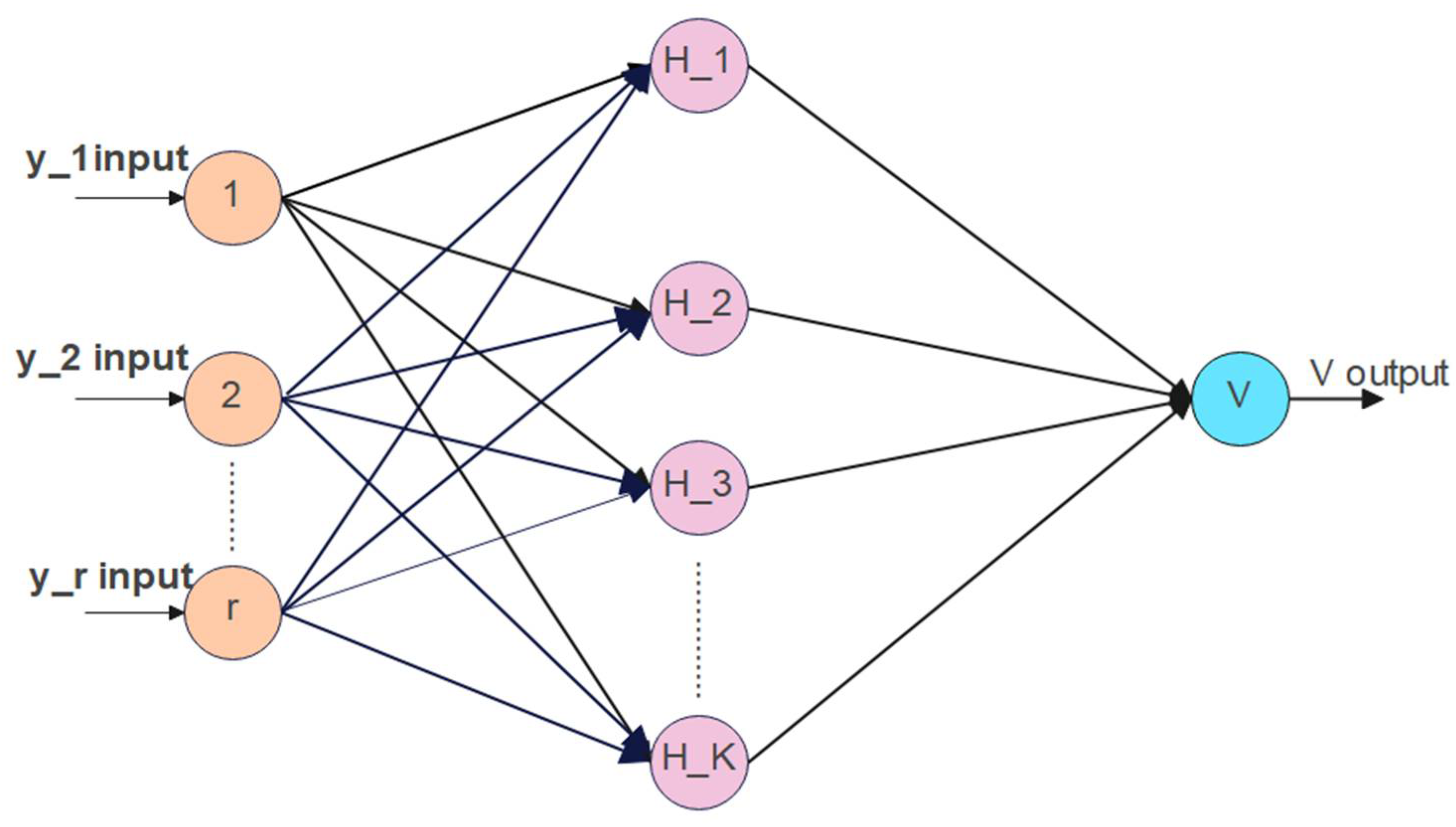
2.1. Extreme Learning Machine

To answer huge and complicated data issues using ELM without running out of memory, the network size should be kept minimal while maintaining acceptable generalization accuracy. Its architecture is shown in Figure 1.

ELM Algorithm

For different samples—(y_r,u_r), in which $y_r=\left[y_{r1},y_{r2},y_{r3},\dots \dots ,y_{ri}\right]T$, $u_r=\left[u_{r1},u_{r2},u_{r3},\dots \dots ,u_{rt}\right]T$are the unified single-layer feed-forward neural network containing the number of hidden layer nodes ($\overline{k}$) and the activation function f(x).

$${{\displaystyle \sum }}_{r=1}^{\overline{k}}{\delta }_{r}f\left(y_r\right)={{\displaystyle \sum }}_{r=1}^{\overline{k}}{\delta }_{r}f\left(w_r{y}_r+d_r\right)=z_s,s=1,2,\dots .k\mathrm{m}$$

(1)

where ${\delta }_r={[{\delta }_{r1}{\delta }_{r2},{\delta }_{r3},\dots \dots {\delta }_{rt}]}^T$ denotes the output weights for connecting the ith hidden node and the output node; $w_r\ast y$denotes the inner product.$w_r={[w_{r1},w_{r2,}\dots ..w_{ri}]}^T$ denotes the weights of the input f(x), which connects the nth hidden node.$d_r$ denotes the deviation of the nth hidden node; f(x) is the activation function, and the output of the hidden nodes is (2).

$$f\left(w_r,d_r,y\right)=f\left(w_r\ast y+d_r\right)$$

(2)

A single-hidden-layer feed-forward neural network containing the number of hidden layer nodes ($\overline{k}$) and the activation function f(r) can approximate the k samples {y_r,b_r} without deviation, namely as in Equation (3).

$${\displaystyle \sum }_s^k\Vert z_s-u_s\Vert =0$$

(3)

The relationship of ${\delta }_r{w}_r,d_r$ is given by (4):

$${\displaystyle \sum }_{r=1}^{\overline{k}}{\delta }_{r}f\left(w_r{y}_s+d_r\right)=u_s,s=1,2,\dots ..k$$

(4)

The above Formula (4) can be represented by the matrix below in (5).

$$\left[v\right]\left[\delta \right]=\left[u\right]$$

(5)

where matrix (6).

$$v\left(w_1,\dots ..,w_{\overline{k}},d_1\dots .,d_{\overline{k}},y_1,\dots .,y_{\overline{k}}\right)={\left|\begin{array}{c}\begin{array}{ccc}f\left(w_1{y}_1+d_1\right)& \dots & f\left(w_{\overline{k}}{y}_1+d_{\overline{K}}\right)\end{array}\\ \dots \\ \begin{array}{ccc}f\left(w_1{y}_N+b_K\right)& \dots & f\left(w_{\overline{K}}{y}_{\overline{K}}{d}_{\overline{K}}\right)\end{array}\end{array}\right|}_{\overline{K}\ast \overline{K}}$$

(6)

where ${\widehat{w}}_r,{\widehat{d}}_r\widehat{\delta }$_r (r = 1, 2, K) denotes the output matrix of the hidden layer (7):

$$\delta ={\left|\begin{array}{c}{\delta }_1^T\\ :\\ {\delta }_{\overline{K}}^T\end{array}\right|}_{{\overline{K}}_{*t}}u={\left|\begin{array}{c}{u}_1^U\\ :\\ u_K^U\end{array}\right|}_{K*t}$$

(7)

The matrix v can adjust network parameters constantly by solving the following minimization problem (8):

$$min\Vert v\delta -u\Vert$$

(8)

The traditional single-layer feedforward network (SLFN) needs to find a set of optimal parameters ${\widehat{w}}_r,{\widehat{d}}_r{\widehat{\delta }}_r$ (r = 1, 2… K) following (9):

$$\Vert v\left(w_1,\dots ..,w_{\overline{k}},d_1\dots .,d_{\overline{k}}\right)\delta -u\Vert =mi{n}_{{\widehat{w}}_r,{\widehat{d}}_r\widehat{\delta }\mathrm{r}}\Vert v\left(w_1,\dots ..,w_{\overline{k}},d_1\dots .,d_{\overline{k}}\right)\delta -u\Vert$$

(9)

2.2. Principal Component Analysis

Principal component analysis is a dimensionality-reduction technique, and its goal is to minimize the data’s dimensionality while preserving as much variety as possible from the original dataset.

Steps to perform PCA are:

(a)

Data standardization

The matrix Y is standardized using the following calculation Formula (10):

$$x_{ij}=\frac{y_{ij}-\overline{y_j}}{\sqrt{var\left(y_j\right)}}$$

(10)

where, Y = {$Y_{ii}$ }, X = {X_ij}, i = 1,2, 3…, n, j = 1,2,3…, p.

$$\overline{y}=\frac{1}{n}{{\displaystyle \sum }}_{i=1}^n{y}_{ij}\mathrm{and}Var\left(y_j\right)=\frac{1}{n-1}{{\displaystyle \sum }}_{i=1}^n(y_{ij}-{\overline{y_j)}}^2$$

(11)

(b)

Calculating covariance matrix

The formula for covariance concerning variance is (12) and (13).

$$Var\left(X\right)=\frac{{{\displaystyle \sum }}_{i=1}^n\left(X_i-X^{\prime }\right)\left(X_i-X^{\prime }\right)}{\left(\mathrm{n}-1\right)}$$

(12)

$$Cov\left(X,Y\right)=\frac{{{\displaystyle \sum }}_{i=1}^n\left(X_i-X^{\prime }\right)\left(Y_i-Y^{\prime }\right)}{\left(\mathrm{n}-1\right)}$$

(13)

• where
• X’ = Arithmetic mean of data X.
• Y’ = Arithmetic mean of data Y.
• $n$ = Number of observations.

The Covariance matrix can be obtained as (14):

$${{\displaystyle \sum }}^{ }=\left[\begin{array}{cc}Var\left(X\right)& Cov\left(x,y\right)\\ Cov\left(Y,X\right)& Var\left(Y\right)\end{array}\right]$$

(14)

The correlation coefficient matrix R is solved as follows (15):

$$R=\frac{X^{T}X}{n-1}$$

(15)

(c)

Eigenvalues are determined by solving

$$\left|\left(S-\lambda I\right)\right|=0$$

(16)

Eigenvectors of ${\lambda }_1$. are given below

$$\left(S-\lambda I\right)U_1=0$$

The eigenvalue and eigenvector of the coefficient matrix are calculated as follows:

$$\left|R-\lambda I_n\right|=0.$$

(17)

The calculated eigenvector is $a_i=\left(a_{i1},a_{i2,}{a}_{i3,}\dots \dots .a_{in}\right),for i=1,2,3\dots ..,n,$ and the eigenvalue is ${\lambda }_i$. Eigenvalues are sorted in descending order to obtain a set of principal components $F_i$, as in (18):

$$F_i=a_{i1}{X}_1+a_{i2}{X}_2+a_{i3}{Y}_3+\dots \dots ..+a_{in}{X}_n$$

(18)

(d)

Choosing new components

The principal components are determined as follows: the rate of contribution of the kth principal component is given as (19):

$${\lambda }_k\left({\displaystyle \sum }_{j=1}^n{\lambda }_j\right)$$

(19)

The rate of the accumulating contribution of the first k principal component is given as (20):

$${\displaystyle \sum }_{j=1}^k{\lambda }_j\left({\displaystyle \sum }_{j=1}^n{\lambda }_j\right)$$

(20)

2.3. PCA–ELM

Figure 2 indicates the approach to the integration of PCA and ELM, which is split into three segments. Segment 1 is the selection of the input dataset. A thermal power plant is built with huge machines and other equipment, where a lot of parameters will affect their efficiency. The efficiency of the machines and equipment affects the efficiency of the thermal power plant. A boiler’s efficiency is purely based on parameters such as the inlet steam pressure, inlet steam temperature, outlet steam pressure, and outlet steam temperature, etc. So, a dataset consisting of the values of these parameters is selected as the input data. The principal component analysis is performed in Segment 2 on the selected input data. The principal components i.e., a new dataset with reduced dimensions, are set as the input to ELM. Segment 3 details ELM development and execution. The new data obtained by Segment 2 is further divided into training and testing datasets. The ELM model is simulated, and errors are calculated.

The testing accuracy of the developed model can be determined from several errors such as the Mean Square Error—mean of the square of the resulted error; Mean Absolute Error—mean of the absolute values of the error; Root Mean Square Error—square root of the mean square error; Mean Absolute Percentage Error—percentage value of the mean absolute error. For K number of samples, the actual and predicted value for each sample u are given by $y_u, {\widehat{y}}_u$, respectively. Then, the errors are determined using Equations (21)–(24). At last, the network model with the least errors is preferable.

$$\mathrm{Mean}\mathrm{Squared}\mathrm{Error}(\mathrm{MSE})=\frac{1}{K}{{\displaystyle \sum }}^{ }{(y_u-{\widehat{y}}_u)}^2$$

(21)

$$\mathrm{Mean}\mathrm{Absolute}\mathrm{Error}(\mathrm{MAE})=\frac{1}{K}{{\displaystyle \sum }}^{ }\left(y_u-{\widehat{y}}_u\right)$$

(22)

$$\mathrm{Root}\mathrm{Mean}\mathrm{Squared}\mathrm{Error}(\mathrm{RMSE})=\sqrt{\frac{1}{K}{{\displaystyle \sum }}^{ }{\left(y_u-{\widehat{y}}_u\right)}^2}$$

(23)

$$\mathrm{Mean}\mathrm{Absolute}\mathrm{Percentage}\mathrm{Error}(\mathrm{MAPE})=\frac{100}{K}{{\displaystyle \sum }}^{ }\left|\frac{y_u-{\widehat{y}}_u}{y_u}\right|$$

(24)

3. Model Approach

This research is based on the boiler consumption at the Yermarus Thermal Power Station (YTPS) located in India. The Yermarus Thermal Power Station is a coal-fired thermal power station in the Raichur district of Karnataka. The Karnataka Power Corporation owns the power facility. Bharat Heavy Electricals is the EPC contractor for this power project, which is India’s first 800 MW supercritical thermal power plant. The plant has two units in it. The installed capacity of the power plant is 1600 MW (2 × 800 MW).

The equipment of a thermal power plant has different operating parameters to generate the maximum capacity. For a boiler, the operating parameters are the inlet steam pressure, inlet steam temperature, outlet steam pressure, outlet steam temperature, at re-heater, super-heater, de-super-heater, air pre heater, forced draft and load, total coal flow, total primary air flow, total secondary air flow, separated overfire air, heavy fuel oil pump current, seal air fan current, Air Pre-Heater (APH) main motor current, and APH standby motor current, and the levels of various gases are the parameters fed as inputs to perform PCA. From the widely deployed measuring devices, sensors, and recorders, the boiler log is summarized. Further, data from this boiler log for January 2022 from the Yermarus thermal power station were given as the input to the network model. It consists of nine coal mills. The data consist of 232 parameters and 96 samples each.

The PCA calculation was performed on SPSS 19.0 software. Upon performing the eigenvalue decomposition technique for the input data covariance matrix, 232 parameters were reduced to 16 principal components based upon the covariance factor. The variance of each parameter can be explained using

Table 1. Variance of the obtained 16 principal components.

Component Number	Eigenvalue	% of Variance	Cumulative %
1	75.245	32.433	32.433
2	54.165	23.347	55.780
3	34.359	14.810	70.590
4	19.495	8.403	78.993
5	11.663	5.027	84.020
6	5.936	2.559	86.579
7	4.683	2.018	88.597
8	3.185	1.373	89.970
9	2.416	1.042	91.012
10	2.184	0.941	91.953
11	1.697	0.731	92.685
12	1.625	0.701	93.385
13	1.550	0.668	94.053
14	1.370	0.591	94.644
15	1.252	0.540	95.184
16	1.056	0.455	95.639

.

For all the 232 variables, there will be 232 components, but the characteristics of the original variables will be reduced to 16 components. Key information about the 232 variables is mined from these components. The percentage of the variance of the first principal component (PC1) is 32.433. It signifies that the first principal component has 32.433% of the characteristics of the original data. The second principal component (PC2) has the second highest variance percentage of 23.347%. These 16 principal components form the inputs to the input layer of the modeled ELM network. The modeling of the ELM includes the selection of the number of hidden neurons and activation function and the division of data for training and testing. The modeled ELM consists of one hidden layer, and a variety of activation functions are considered. All the data are divided into two parts—one part is for training, and the other for testing. The ELM model is built for predicting the output. First, the ELM has been trained on some samples by giving both inputs and outputs. After that, it has been tested on some inputs, and the outputs obtained are compared with the original outputs in the data.

The PC1 vs PC2 results are depicted in Figure 3. The type of activation function and number of hidden neurons affect the prediction capability and speed of the ELM model. If the accuracy and speed of the model is good, then the network model can be used for further greater analysis. By using SPSS, the principal components are randomly assigned as training samples and testing samples for different ranges of hidden nodes (i.e., 3, 30, 50, 80, 100) and activation functions (sigmoid and hyperbolic tangent) when the PCA–ELM model is stimulated and tested.

4. Results and Discussion

To determine the best approach between ELM and PCA–ELM, initially, the dataset of 232 variables and 96 samples is standardized. Then, principal component analysis is performed, and the spread of the obtained components can be observed in Figure 4. The first 16 components have a greater percentage of the variance than the rest of the components, meaning all the characteristics of the original dataset are present in those 16 principal components.

From Table 1 the percentage variance of the obtained 16 principal components is as follows: 32.4, 23.3, 14.8, 8.4, 5.02, 2.5, 2.01, 1.3, 1.04, 0.94, 0.73, 0.701, 0.668, 0.59, 0.54, 0.455, and the cumulative contribution rate is 95.639%. It signifies that the 16 principal components represent 95.639% of the original dataset characteristics. A conventional ELM model using a sigmoid activation function with 50 hidden nodes is developed, and the original data of 232 variables is given as training and testing samples.

In the next part of the simulation, the dimensionality of the huge input data is reduced using PCA and then integrated into ELM, continuing with the same ELM design of a sigmoid activation function and 50 hidden nodes. A comparison of the predictions using both the approaches—ELM and PCA–ELM, during training and testing—consists of 2 general parts: relative errors and training time.

Results shown in

Table 2. ELM model and PCA–ELM integration model using a sigmoid activation function with 50 hidden neurons.

Parameters/Approach	ELM	PCA–ELM
training sum of squares error	0.02	0.015
training time (in milliseconds)	13	2
training relative error	0.009	0.01
the testing sum of squares error	0.05	0.023
testing relative error	0.065	0.017
MSE	39.932	14.711
MAE	3.902	2.969
MAPE	0.696	0.526
RMSE	6.319	3.835

highlight that the conventional ELM model takes 13 ms, whereas PCA–ELM takes only 2 ms.

More time for training and the relative errors are high compared to the PCA–ELM integrated model, and the cause of high-dimensional data can be observed on a network model. So, the PCA–ELM integrated model has the best prediction capability and is more accurate towards training time. In addition, the ELM and PCA–ELM models using a sigmoid activation function with 100 hidden nodes are developed. From

Table 3. ELM model and PCA–ELM integration model using a sigmoid activation function with 100 hidden neurons.

Parameters/Approach	ELM	PCA–ELM
training sum of squares error	0.002	0.015
training time (in milliseconds)	45	2
training relative error	0.001	0.01
testing sum of squares error	0.038	0.023
testing relative error	0.053	0.017
MSE	25.269	22.380
MAE	2.726	3.626
MAPE	0.481	0.639
RMSE	5.026	4.730

, the relative errors and training time for both the models can be observed.

Now, an accurate prediction model is established, but the choice of the number of hidden nodes and activation functions is a failing factor. To begin, PCA–ELM models using a sigmoid activation function with different ranges of hidden neurons of 3, 30, 50, 80, and 100 were created, with mean square errors of 160, 23, 14, 33, and 22 respectively. From

Table 4. Sigmoid-function-based PCA–ELM model for a various number of hidden neurons.

Parameter/Model	S-3	S-30	S-50	S-80	S-100
training sum of squares error	0.094	0.022	0.015	0.018	0.015
training time (in milliseconds)	0	0	2	2	2
training relative error	0.045	0.012	0.01	0.013	0.01
testing sum of squares error	0.158	0.018	0.023	0.034	0.023
testing relative error	0.278	0.018	0.017	0.027	0.017
MSE	160.063	23.487	14.714	33.224	22.379
MAE	8.0185	3.531	2.969	4.282	3.626
MAPE	1.436	0.621	0.526	0.767	0.639
RMSE	12.655	4.841	3.835	5.764	4.730

, the results show that the prediction model using the sigmoid function should be implemented with a high range of hidden nodes (mostly 30 or more hidden nodes).

PCA–ELM models using a hyperbolic tangent activation function with different ranges of hidden neurons of 3, 30, 50, 80, and 100 are developed, and the mean square errors of the models are 107, 42, 61, 110, and 668, respectively. From Table 4 and

Table 5. Hyperbolic-tangent-function-based PCA–ELM model for a various numbers of hidden neurons.

Parameter/Model	H-3	H-30	H-50	H-80	H-100
training sum of squares error	0.288	0.021	0.008	0.125	2.268
training time (in milliseconds)	2	2	6	5	9
training relative error	0.037	0.002	0.001	0.025	0.288
testing sum of squares error	0.386	0.272	0.415	0.733	1.939
testing relative error	0.135	0.019	0.135	0.094	0.678
MSE	107.124	42.206	61.051	110.047	668.565
MAE	7.249	3.200	3.141	6.609	21.095
MAPE	1.300	0.572	0.557	1.180	3.668
RMSE	10.350	6.496	7.813	10.490	25.857

, in the case of 30 hidden nodes, the MSE is 23.487 with the sigmoid-function-based PCA–ELM model, whereas it is 42.206 with the hyperbolic-tangent-function-based PCA–ELM model. In the case of 100 hidden neurons, the MSE is 22.379 with the sigmoid-function-based PCA–ELM model, whereas it is 668.565 with the hyperbolic-tangent-function-based PCA–ELM model. This shows that the prediction model using the sigmoid function is more reliable from the lower range of hidden nodes.

The Mean Absolute Error (MAE), Mean Absolute Percentage Error (MAPE), and Root Mean Square Error (RMSE) are determined from the predicted values. An extensive comparison of these values for various numbers of hidden nodes and both activation functions —hyperbolic tangent and sigmoid functions—is illustrated in Figure 5. Notations used in Figure 5 represent activation function-number of neurons, where ‘H’, ‘S’ represent the hyperbolic tangent function and sigmoid function, respectively. For example, H-3—represents a hyperbolic tangent activation function with 3 hidden neurons, and S-3—a sigmoid activation function with 3 hidden neurons.

The developed PCA–ELM network’s workings have been tested in three aspects:

• The performance of the conventional ELM has been compared with that of PCA–ELM.
• The PCA–ELM network was compared by varying the range of hidden neurons.
• The two PCA–ELM networks using the hyperbolic tangent function and sigmoid function are developed and compared.

The PCA–ELM network was built using the hyperbolic tangent function, and the range of neurons is varied. As the range of neurons increased, the error also increased, and the efficiency of the model decreased, whereas in the PCA–ELM network using a sigmoid function when the range of hidden neurons is varied, as the range is increased, the error decreased. The number of hidden neurons is varied from 3, 30, 50, 80, and 100. In addition, the training time for a neural network model is crucial, and a conventional ELM network is challenging. So, by using the PCA technique, the large boiler data are reduced to minimal data without losing any of their features, and those acquired principal components are integrated into the ELM network; this PCA–ELM is accurate and fast compared to the conventional ELM network. This can be observed from training time in the comparison

Table 6. PCA–ELM models using a hyperbolic tangent function and sigmoid function with different ranges of hidden neurons.

H/S	H	H	H	H	H	S	S	S	S	S
Number of hidden neurons	3	30	50	80	100	3	30	50	80	100
training sum of squares error	0.288	0.021	0.008	0.125	2.268	0.094	0.022	0.015	0.018	0.015
training time (ms)	2	2	6	5	9	0	0	2	2	2
training relative error	0.037	0.002	0.001	0.025	0.288	0.045	0.012	0.01	0.013	0.01
testing sum of squares error	0.386	0.272	0.415	0.733	1.939	0.158	0.018	0.023	0.034	0.023
testing relative error	0.135	0.019	0.135	0.094	0.678	0.278	0.018	0.017	0.027	0.017
MSE	107.12	42.206	61.051	110.04	668.56	160.063	23.487	14.711	33.224	22.3799
MAE	7.2494	3.2004	3.1415	6.6091	21.095	8.01854	3.5317	2.9691	4.2829	3.62697
MAPE	1.3001	0.5720	0.5574	1.1800	3.6681	1.43662	0.6339	0.5260	0.7671	0.63997
RMSE	10.35008	6.496684	7.813519	10.49037	25.85701	12.6516305	4.846391	3.835549	5.764049	4.73075014

.

5. Conclusions

In this paper, a combined approach of principal component analysis with extreme learning machines is investigated to predict boiler output power in a thermal power plant. The electrical output of a boiler in the operating system requires knowledge of 232 operating parameters. Principal component analysis is performed to reduce the dimensionality of the input dataset. These principal components form the input matrix for the extreme learning machine. Total inputs are divided into two parts—training and testing datasets. To validate the effectiveness of the combined approach of PCA–ELM, it is compared with ELM in terms of its testing accuracy and simulation time. Further, the ELM model is designed with various activation functions and several hidden neurons, and the results for simulation time and testing accuracy are compared. In summary, according to the predictions made, the following conclusions can be drawn:

i.

To predict the boiler output power in a thermal power plant, PCA–ELM is superior to ELM in predicting accuracy and learning speed. This is because with PCA, the dimension of the inputs is reduced while maintaining the properties of the data points using variance, thereby reducing the computation time.

ii.

In terms of prediction precision, PCA–ELM shows superior performance over ELM because of the eigenvalue decomposition technique for the input data covariance matrix. In this way, correlated input parameters are carefully converted into linearly uncorrelated ones. Thus, this shows the necessity for dimensionality reduction methods to enhance forecasting.

iii.

The generalization ability of the ELM is corroborated with changes in ELM parameters’ activation function and the number of hidden nodes. In a comparison of PCA–ELM models with a hyperbolic tangent function and those with a sigmoid function, the latter shows better performance in terms of errors. However, the performance of the hyperbolic tangent function deteriorates with the increasing number of hidden neurons.

This paper primarily studies the forecasting of boiler output based on thermal power plant operating parameters. It can further be extended to the optimization of the input parameters. For the fact of serious air pollution caused by thermal plants, these outcomes may also be considered in the production planning. Hence there are numerous other ways to incorporate this study.

References

1. Vom Scheidt, F.; Medinová, H.; Ludwig, N.; Richter, B.; Staudt, P.; Weinhardt, C. Data analytics in the electricity sector—A quantitative and qualitative literature review. Energy AI 2020, 1, 100009. [Google Scholar] [CrossRef]
2. Bhangu, S.N.; Singh, R.; Pahuja, G.L. Availability performance analysis of thermal power plants. J. Inst. Eng. India Ser. C 2019, 100, 439–448. [Google Scholar] [CrossRef]
3. Tüfekci, P. Prediction of full load electrical power output of a base load operated combined cycle power plant using machine learning methods. Int. J. Electr. Power Energy Syst. 2014, 60, 126–140. [Google Scholar] [CrossRef]
4. Lorencin, I.; Anđelić, N.; Mrzljak, V.; Car, Z. Genetic Algorithm Approach to Design of Multi-Layer Perceptron for Combined Cycle Power Plant Electrical Power Output Estimation. Energies 2019, 12, 4352. [Google Scholar] [CrossRef] [Green Version]
5. Kesgin, U.; Heperkan, H. Simulation of thermodynamic systems using soft computing techniques. Int. J. Energy Res. 2005, 29, 581–611. [Google Scholar] [CrossRef]
6. Ma, J.; Xia, D.; Guo, H.; Wang, Y.; Niu, X.; Liu, Z.; Jiang, S. Metaheuristic-based support vector regression for landslide displacement prediction: A comparative study. Landslides 2022, 1–23. [Google Scholar] [CrossRef]
7. Ma, J.; Wang, Y.; Niu, X.; Jiang, S.; Liu, Z. A comparative study of mutual information-based input variable selection strategies for the displacement prediction of seepage-driven landslides using optimized support vector regression. Stoch. Hydrol. Hydraul. 2022, 1–21. [Google Scholar] [CrossRef]
8. Dong, Y.; Gu, Y.; Yang, K.; Zhang, J. Applying PCA to establish artificial neural network for condition prediction on equipment in power plant. In Proceedings of the Fifth World Congress on Intelligent Control and Automation (IEEE Cat. No.04EX788), Shenyang, China, 15–19 June 2004; Volume 2, pp. 1715–1719. [Google Scholar] [CrossRef]
9. Fei, W.; Mi, Z.; Shi, S.; Zhang, C. A practical model for single-step power prediction of grid-connected PV plant using artificial neural network. In Proceedings of the 2011 IEEE PES Innovative Smart Grid Technologies, Perth, WA, Australia, 13–16 November 2011; pp. 1–4. [Google Scholar] [CrossRef]
10. Mei, R.; Lv, Z.; Tang, Y.; Gu, W.; Feng, J.; Ji, J. Short-term prediction of wind power based on principal component analysis and Elman neural network. In Proceedings of the 2021 IEEE Sustainable Power and Energy Conference (iSPEC), Nanjing, China, 23–25 December 2021; pp. 3669–3674. [Google Scholar] [CrossRef]
11. Ma, L.; Wang, X.; Cao, X. Feedwater heater system fault diagnosis during dynamic transient process based on two-stage neural networks. In Proceedings of the 32nd Chinese Control Conference, Xi’an, China, 26–28 July 2013; pp. 6148–6153. [Google Scholar]
12. Chen, G.; Shan, J.; Li, D.Y.; Wang, C.; Li, C.; Zhou, Z.; Wang, X.; Li, Z.; Hao, J.J. Research on Wind Power Prediction Method Based on Convolutional Neural Network and Genetic Algorithm. In Proceedings of the 2019 IEEE Innovative Smart Grid Technologies—Asia (ISGT Asia), Chengdu, China, 21–24 May 2019; pp. 3573–3578. [Google Scholar] [CrossRef]
13. Dong, Y.; Ma, X.; Fu, T. Electrical load forecasting: A deep learning approach based on K-nearest neighbors. Appl. Soft Comput. 2020, 99, 106900. [Google Scholar] [CrossRef]
14. Malhotra, R. Comparative analysis of statistical and machine learning methods for predicting faulty modules. Appl. Soft Comput. 2014, 21, 286–297. [Google Scholar] [CrossRef]
15. Zhou, H.; Huang, G.; Lin, Z.; Wang, H.; Soh, Y.C. Stacked extreme learning machines. IEEE Trans. Cybern. 2014, 45, 2013–2025. [Google Scholar] [CrossRef]
16. Huang, G.-B.; Zhou, H.; Ding, X.; Zhang, R. Extreme Learning Machine for Regression and Multiclass Classification. IEEE Trans. Syst. Man Cybern. Part B Cybern. 2012, 42, 513–529. [Google Scholar] [CrossRef] [PubMed] [Green Version]
17. Huang, G.-B.; Zhu, Q.; Mao, K.Z.; Siew, C.; van Saratchandran, P.; Sundararajan, N. Can threshold networks be trained directly? IEEE Trans. Circuits Syst. II Express Briefs 2006, 53, 187–191. [Google Scholar] [CrossRef]
18. Miche, Y.; Sorjamaa, A.; Lendass, A. OP-ELM: Theory, experiments and a toolbox. In International Conference on Artificial Neural Networks; Springer: Berlin/Heidelberg, Germany, 2008; pp. 145–154. [Google Scholar]
19. Tan, P.; Xia, J.; Zhang, C.; Fang, Q.; Chen, G. Modeling and reduction of NOX emissions for a 700 MW coal-fired boiler with the advanced machine learning method. Energy 2015, 94, 672–679. [Google Scholar] [CrossRef]
20. Zhao, H.; Zhao, J.; Zheng, Y.; Qiu, J.; Wen, F. A Hybrid Method for Electric Spring Control Based on Data and Knowledge Integration. IEEE Trans. Smart Grid 2019, 11, 2303–2312. [Google Scholar] [CrossRef]
21. Shi, X.; Kang, Q.; An, J.; Zhou, M. Novel L1 Regularized Extreme Learning Machine for Soft-Sensing of an Industrial Process. IEEE Trans. Ind. Inform. 2021, 18, 1009–1017. [Google Scholar] [CrossRef]
22. Yu, H.; Yang, L.; Zhou, Y. Navigation System Research and Design Based on Intelligent Image Classification Algorithm of Extreme Learning Machine. In Proceedings of the 2020 IEEE International Conference on Power, Intelligent Computing and Systems (ICPICS), Shenyang, China, 28–30 July 2020; pp. 930–933. [Google Scholar] [CrossRef]
23. Patnaik, S.; Tripathy, L.; Dhar, S. An Improved Water Cycle Optimized Extreme Learning Machine with Ridge Regression towards Effective Maximum Power Extraction for Photovoltaic based Active Distribution Grids. In Proceedings of the 2020 International Conference on Computational Intelligence for Smart Power System and Sustainable Energy (CISPSSE), Keonjhar, Odisha, 23–35 April 2020; pp. 1–6. [Google Scholar] [CrossRef]
24. Giri, M.K.; Majumder, S. Extreme Learning Machine Based Cooperative Spectrum Sensing in Cognitive Radio Networks. In Proceedings of the 2020 7th International Conference on Signal Processing and Integrated Networks (SPIN), Noida, India, 27–28 February 2020; pp. 636–641. [Google Scholar] [CrossRef]
25. Tang, Z.; Wang, S.; Chai, X.; Cao, S.; Ouyang, T.; Li, Y. Auto-encoder-extreme learning machine model for boiler NOx emission concentration prediction. Energy 2022, 256, 124552. [Google Scholar] [CrossRef]
26. Mishra, P.S.; Sarkar, U.; Taraphder, S.; Datta, S.; Swain, D.; Saikhom, R.; Panda, S. MenalshLaishramMultivariate statistical data analysis-principal component analysis (PCA). Int. J. Livest. Res. 2017, 7, 60–78. [Google Scholar]
27. Yang, J.; Zhang, D.; Frangi, A.; Yang, J.-Y. Two-dimensional pca: A new approach to appearance-based face representation and recognition. IEEE Trans. Pattern Anal. Mach. Intell. 2004, 26, 131–137. [Google Scholar] [CrossRef] [Green Version]
28. Gottumukkal, R.; Asari, V.K. An improved face recognition technique based on modular PCA approach. Pattern Recognit. Lett. 2004, 25, 429–436. [Google Scholar] [CrossRef]
29. Draper, B.A.; Baek, K.; Bartlett, M.S.; Beveridge, J. Recognizing faces with PCA and ICA. Comput. Vis. Image Underst. 2003, 91, 115–137. [Google Scholar] [CrossRef]
30. Daffertshofer, A.; Lamoth, C.J.; Meijer, O.G.; Beek, P.J. PCA in studying coordination and variability: A tutorial. Clin. Biomech. 2004, 19, 415–428. [Google Scholar] [CrossRef] [PubMed]
31. Choi, S.W.; Lee, C.; Lee, J.-M.; Park, J.H.; Lee, I.-B. Fault detection and identification of nonlinear processes based on kernel PCA. Chemom. Intell. Lab. Syst. 2005, 75, 55–67. [Google Scholar] [CrossRef]
32. Yu, J.; Yoo, J.; Jang, J.; Park, J.H.; Kim, S. A novel plugged tube detection and identification approach for final super heater in thermal power plant using principal component analysis. Energy 2017, 126, 404–418. [Google Scholar] [CrossRef]
33. Ferracuti, F.; Giantomassi, A.; Ippoliti, G.; Longhi, S. Multi-Scale PCA Based Fault Diagnosis for Rotating Electrical Machines. In Proceedings of the European Workshop on Advanced Control and Diagnosis, 8th ACD, Ferrara, Italy, 18–19 November 2010; pp. 296–301. [Google Scholar]
34. Filho, J.M.; Filho, J.M.D.C.; Paiva, A.P.; de Souza, P.V.G.; Tomasin, S. A PCA-based approach for substation clustering for voltage sag studies in the Brazilian new energy context. Electr. Power Syst. Res. 2016, 136, 31–42. [Google Scholar] [CrossRef]
35. Bhutto, J.A.; Lianfang, T.; Du, Q.; Soomro, T.A.; Lubin, Y.; Tahir, M.F. An Enhanced Image Fusion Algorithm by Combined Histogram Equalization and Fast Gray Level Grouping Using Multi-Scale Decomposition and Gray-PCA. IEEE Access 2020, 8, 157005–157021. [Google Scholar] [CrossRef]
36. Serna, I.; Morales, A.; Fierrez, J.; Obradovich, N. Sensitive loss: Improving accuracy and fairness of face representations with discrimination-aware deep learning. Artif. Intell. 2022, 305, 103682. [Google Scholar] [CrossRef]
37. Castaño, A.; Fernández-Navarro, F.; Hervás-Martínez, C. PCA-ELM: A robust. Neural Processing Lett. 2013, 37, 377–392. [Google Scholar] [CrossRef]
38. Miao, Y.Z.; Ma, X.P.; Bu, S.P. Research on the Learning Method Based on PCA-ELM. Intell. Autom. Soft Comput. 2017, 23, 637–642. [Google Scholar] [CrossRef]
39. Ji, Y.; Zhang, S.; Yin, Y.; Su, X. Application of the improved the ELM algorithm for prediction of blast furnace gas utilization rate. IFAC-PapersOnLine 2018, 51, 59–64. [Google Scholar] [CrossRef]
40. Yuan, B.; Wang, W.; Ye, D.; Zhang, Z.; Fang, H.; Yang, T.; Wang, Y.; Zhong, S. Nondestructive Evaluation of Thermal Barrier Coatings Thickness Using Terahertz Technique Combined with PCA–GA–ELM Algorithm. Coatings 2022, 12, 390. [Google Scholar] [CrossRef]
41. Sun, W.; Sun, J. Prediction of carbon dioxide emissions based on principal component analysis with regularized extreme learning machine: The case of China. Environ. Eng. Res. 2017, 22, 302–311. [Google Scholar] [CrossRef] [Green Version]
Figure 1. Extreme learning machine architecture.
Applsci 12 07671 g001
Figure 2. PCA–ELM Integration Approach.
Applsci 12 07671 g002
Figure 3. Principal component 1 vs. principal component 2.
Applsci 12 07671 g003
Figure 4. Scree plot explaining the spread of principal components.
Applsci 12 07671 g004
Figure 5. Comparison of the errors for various models.
Applsci 12 07671 g005