CO₂ Distribution under CO₂ Enrichment Using Computational Fluid Dynamics Considering Photosynthesis in a Tomato Greenhouse

Abstract

This study validated the CO₂ distribution predicted by a computational fluid dynamics model considering CO₂ absorption by photosynthesis in a chamber and greenhouse. The effect of photosynthesis with CO₂ emission from a perforated tube remains not fully understood, although previous studies on CO₂ distribution in greenhouses have been conducted. Moreover, comparisons between CO₂ concentration measurement and simulation were obtained in the chamber and greenhouse model. Cases with open and closed side vents of the greenhouse showed that closed side vents have slightly more even of CO₂ concentration than those with open side vents inside the greenhouse. In contrast, the coefficient of variance (CV) of CO₂ inside the plant, open (8.8%) and closed (8.7%) side vents, induced almost no significant improvement. Additionally, cases of a rainy- and sunny-day model showed that photosynthetically active radiation possibly compensated CO₂ absorption through photosynthesis to be low at low light (rainy day) and higher at high light (sunny day). Nonetheless, the variability of CO₂ concentration inside the plant between rainy and sunny days determined almost no significant difference. Thus, this research shows characteristics of CO₂ distribution, assessing photosynthesis and the variability of CO₂ concentration that leads to the efficiency of CO₂ enrichment in the greenhouse.

1. Introduction

Extending the farmland and improving production inside the greenhouse are two strategies expected to boost agricultural productivity. Many researchers have studied the microclimate phenomena of greenhouses because of the increasing demand for value-added agricultural products and the efficacy area of the greenhouse [1,2,3]. However, previous studies focused on the relationship between climatic factors that affect crop development [4,5,6,7]. In contrast, only a few studies have investigated the CO₂ distribution [8,9,10,11].

CO₂ enrichment is one of methods used to increase and distribute the CO₂ concentration near to the plant. This method is conducted by controlling and maintain CO₂ concentration inside the greenhouse [11]. It is challenging to maintain an optimal CO₂ concentration inside a greenhouse because CO₂ is affected by temperature, humidity, and light intensity, resulting in ambient CO₂ concentrations that are either suboptimal or excessive [12].

For example, Kuroyanagi et al. [13] investigated the amount of CO₂ that leaked from an unventilated greenhouse enriched with CO₂ on short-term (hourly) and medium-term investigation. The average short-term CO₂ efficiency by crop absorption was 57.3% during the four days of daylight. For the medium term, more than 27 days, the efficiency of CO₂ enrichment was 45.5% on an average. The investigation demonstrated that the efficiency was not solely caused by the low levels of solar radiation or strong wind. In comparison, higher efficiency was achieved by higher solar radiation and weaker external wind.

Since CO₂ could not be homogeneously spread far from the CO₂ tube (CO₂ source), CO₂ distribution depends on air circulation inside the greenhouse. Thus, the delivery system (air circulation and ventilation) must be designed to ensure an even distribution throughout the greenhouse. Additionally, Kim et al. [14] showed that unequal distribution of CO₂ depends on temperature and location. A comparison showed that temperature is inversely proportional to the change in CO₂ distribution. As mentioned above, CO₂ enrichment plays a significant role in stable crop yield. Nevertheless, the detailed spatiotemporal distribution of CO₂ in foliage remains unknown.

Most of time, chambers are used in experiments to readily regulate environmental conditions because of their comparatively simple design. In this study, the performance of a recently constructed photosynthesis model for CO₂ distribution was assessed using a photosynthetic chamber with exhaust fans on top of the chamber. The new chamber is a semi-closed hanging type chamber covering the entire plant and monitoring the real-time photosynthetic rate.

The new chamber is shaped vertically because it is intended to completely cover plants, such as tomatoes. Shimomoto et al. [15] successfully tracked the time courses of tomato plants, the net photosynthetic rate, transpiration rate, and total conductance inside a monitoring system using a similar chamber. However, since measurement was conducted only for the photosynthetic rate and related environmental factors, the CO₂ distribution in the chamber was not well known.

Computational fluid dynamics (CFD) has been applied in various research areas to predict and simulate a similar process close to the actual condition. Many researchers have analyze greenhouse designs, airflow, temperature, and radiation distribution in the agricultural field using CFD [16,17,18,19,20,21]. Analysis of the detailed CO₂ distribution is rarely implemented and is still ongoing to date. Zhang et al. [11] showed that the efficiency of CO₂ distribution using CO₂ supplement/tube could save half of the fuel and achieve a higher CO₂ concentration compared with a CO₂ generator.

CFD is a powerful tool for describing greenhouse microclimate, plant behavior [22], and photosynthesis. Molina-Aiz et al. [9] reported that photosynthesis could be simulated accurately using CFD in each cell of the domain corresponding to the crop. In their study, photosynthesis was computed as a function of the CO₂ concentration estimated by the CFD software. The CFD model made it possible to reveal airflow details above and within the canopy, effects of the different structures on water irrigation, and predicted crop transpiration [23,24,25].

The validity of the CFD results has been a perennial problem. However, the continuous development of computer and numerical methods enhances the accuracy of the simulation prediction and shows outstanding potential for analyzing complex airflow in a greenhouse [20]. Although photosynthesis has been considered in a recent CFD model, analysis of CO₂ distribution by CO₂ enrichment and emitted by CO₂ supplement/tube is insufficient. Since this research is rarely conducted, this study focuses on finding detailed CO₂ distribution concerning the increased efficiency of photosynthesis.

The objective of this study is to reveal the detailed CO₂ distribution using a CFD model considering photosynthesis with CO₂ enrichment using CO₂ supplement/tube inside the greenhouse. First, the effectiveness of the model is assessed by comparing numerical simulations and measuring the CO₂ levels in the new chamber.

In the chamber simulation, the photosynthesis model is considered to simulate CO₂ absorption, and reasonable results for the model performance are obtained. Finally, the simulated CO₂ content is verified, and the photosynthesis model is used to calculate the precise CO₂ distribution with CO₂ enrichment inside the greenhouse. A few greenhouse simulations are conducted to determine the impact of various environmental factors on the distribution of CO₂ inside of the greenhouse, including side vents that can be open or closed and weather conditions that can be sunny or rainy.

2. Materials and Methods

2.1. Experimental Set-Up

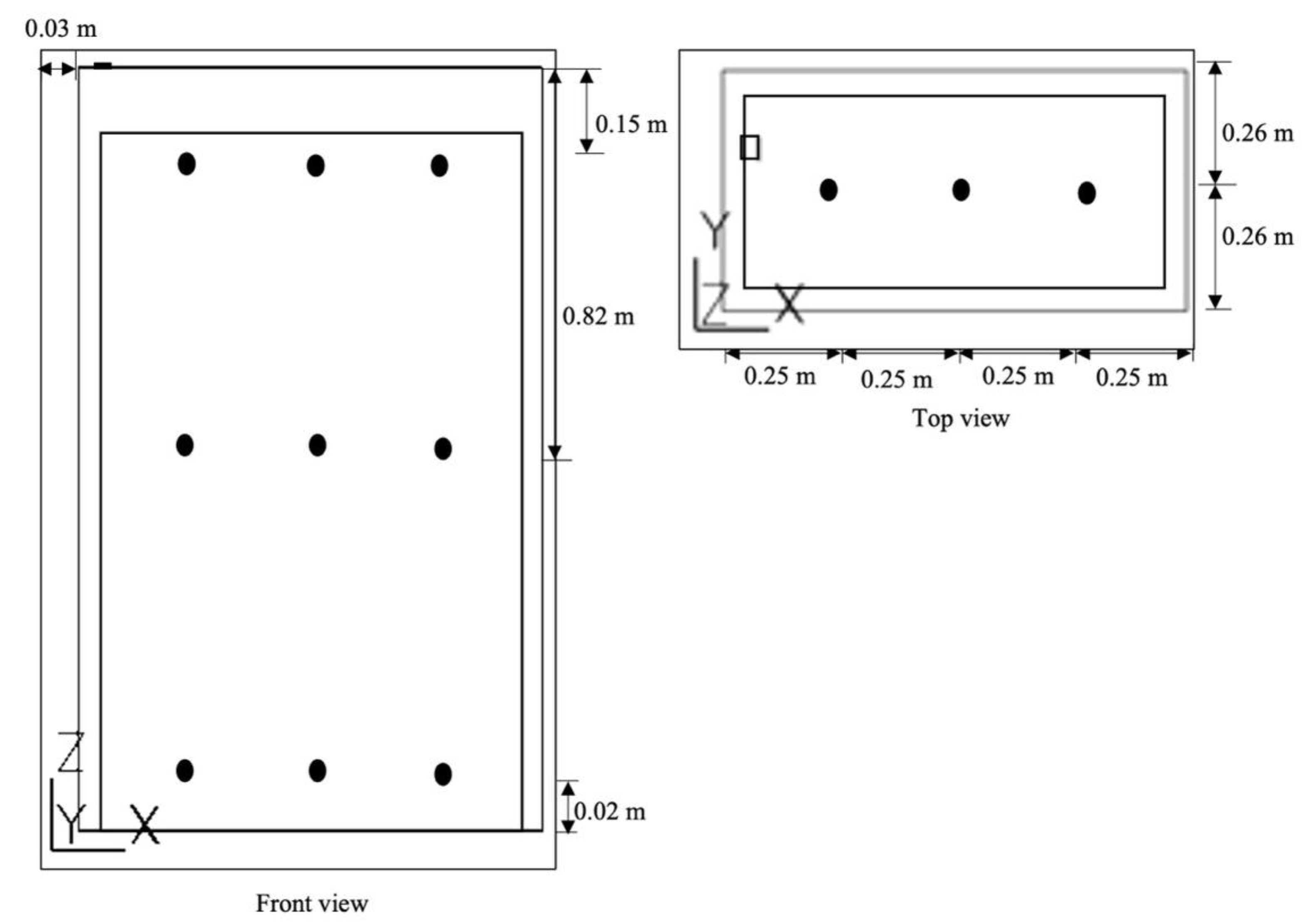
2.1.1. Chamber Description

The experiment was conducted in a chamber inside the greenhouse with a CO₂ concentration of approximately 420 ppm. The chamber is a semi closed hanging type that is 1 m in length, 0.52 m in width, 1.64 m in height, and an area of the bottom opening: 0.52 m² (1 m in length × 0.52 m in width) (Figure 1). The air inside the chamber flows out through an exhaust fan (9BMB24P2H01, Sanyo Denki, Philippines) at the left ceiling of the chamber. The air velocity of the fan is 18.7 m s⁻¹, applied to determine the volumetric flow rate of the fan in this research and used in the simulation as shown below (Equation (1)):

$$Q=u_{\mathrm{out}}\times A_{\mathrm{out}}$$

(1)

where u_out is the air velocity at the exhaust fan boundary (m s⁻¹), Q is the outlet volumetric flow rate (m³ s⁻¹), and A_out is the outlet opening area (m²).

Two whole-grown tomatoes were placed inside the chamber in the substrate with a drip nutrient and irrigation system. The tomatoes had heights of 1.63 and 1.4 m, respectively, from the chamber bottom; leaf area index (LAI) of 4 m² m⁻²; and leaf area density (LAD) of 2.67 m² m⁻³. Later, in the chamber model validation, the average height of 1.5 m was used to represent the height of the plant.

2.1.2. CO₂ Distribution Measurement in the Chamber

CO₂ concentrations were measured using a handheld CO₂ m (GM70, probe type GMP 222, range 0–5000 ppm, accuracy: ±1.5% of range +2% of reading, Vaisala, Finland). The measurements of CO₂ concentration without CO₂ enrichment were conducted in three positions: top (0.15 m from the chamber ceiling), middle (0.815 m from the chamber ceiling), and bottom (at the bottom opening of the chamber) to obtain CO₂ distribution data for model validation. CO₂ concentration at each position was measured in three horizontal points (left, middle, and right) in the exact distance between the point is 0.25 m.

The CO₂ concentration at each point were measured with the CO₂ m held by hand and recorded manually to a sheet when the value displayed on the CO₂ m was stable. However, the CO₂ concentration of the top positions were measured at the left and right because of difficulty reaching the middle point while avoiding human breath exhaling CO₂. Air velocities were measured at the bottom of the chamber (0.83 m from the ground) and 0.2, 0.4, and 0.815 m from the ceiling of the chamber, using a hot wire anemometer (WGT 10, Hario, Japan) to determine the airflow and CO₂ distribution (Figure 2).

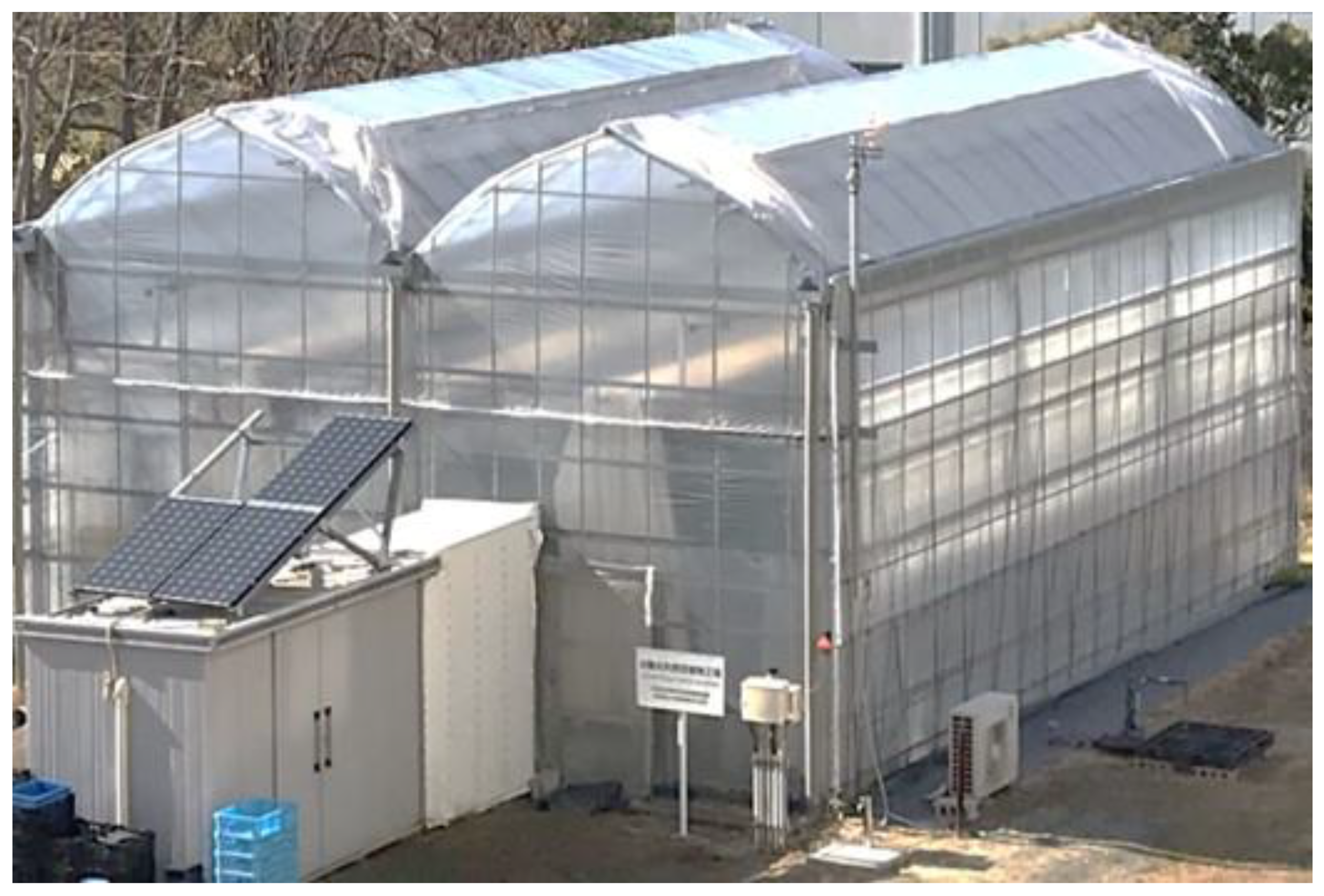
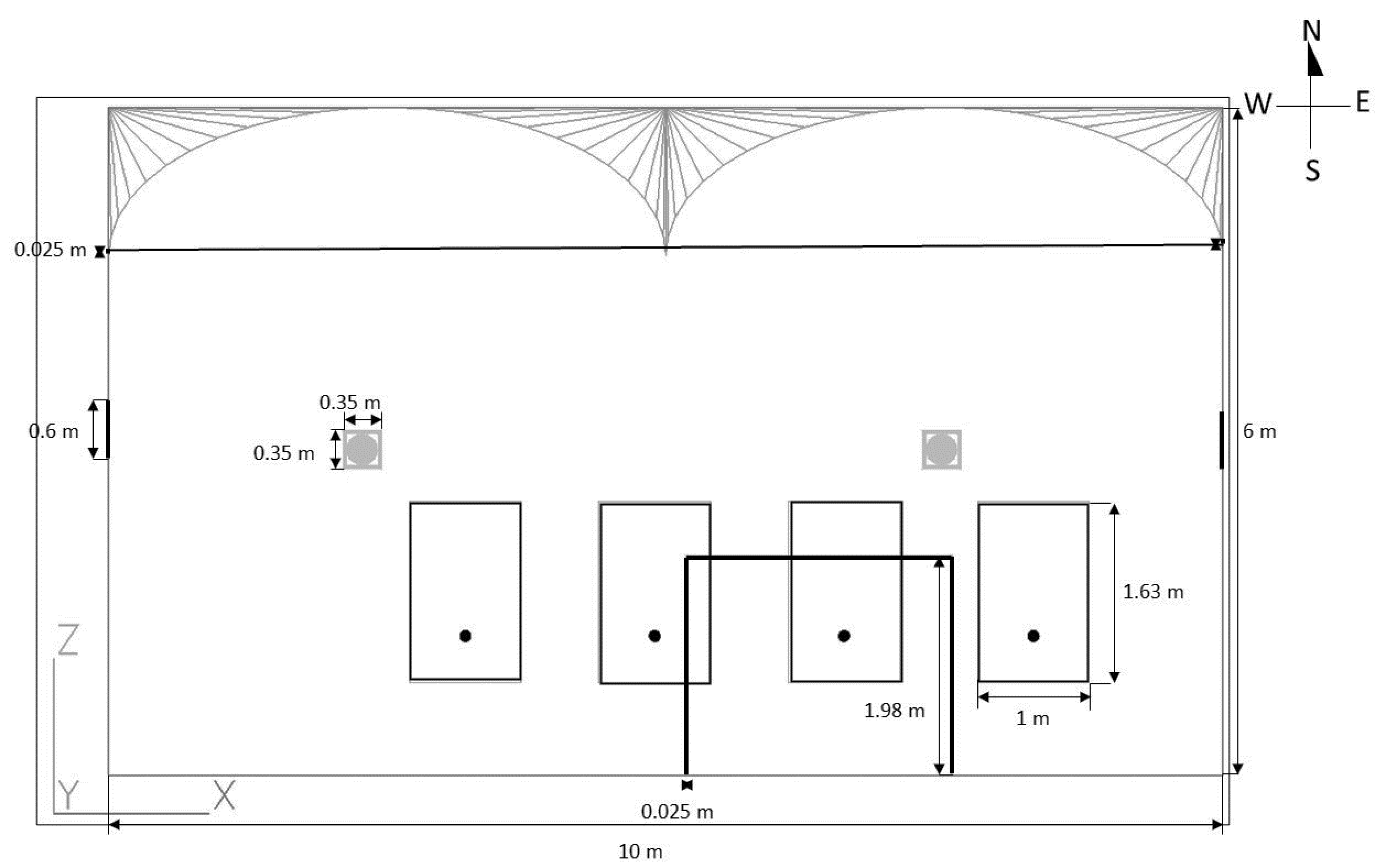
2.1.3. Greenhouse Description

This study was conducted in a vinyl greenhouse of 120 m² (length: 12 m; width: 10 m; height: 6.03 m) located at Toyohashi University of Technology, Japan (Figure 3). The greenhouse was equipped with air conditioning, air circulators, roof and side vents, water and nutrient solution drip-irrigation system, and a perforated tube of airflow system placed above the bed of plants shelves. Additionally, the greenhouse’s roof and side vents were covered with insect-proof nets.

Tomatoes were grown on four shelves inside the greenhouse: tomato seedlings (Solanum lycopersicum), cv. ‘Momotaro hope’, was planted on 4 November 2020, in greenhouse. Tomatoes grow in the cultivated bed (0.23 m in width and 8 m in length), mounting 0.83 m from the ground floor. The water and nutrient solution supply are controlled using monitoring instruments (Aqua beat, Inochio, Japan). The solar radiation data were acquired from the NEDO database (New Energy and Industrial Technology Development Organization, Japan) to calculate PAR (Photosynthetically Active Radiation).

2.1.4. Measurement of CO₂ Concentration in Greenhouse

CO₂ enrichment was conducted during the daytime on a sunny day (on 30 August 2021, at 1.30 p.m.). The initial CO₂ concentration injection was 1160 ppm. Pure CO₂ gas was supplied through a perforated tube airflow system placed in the middle of the bed of plants for each shelf. The perforated tube has a length of 8 m, a diameter of 0.10 m, and 16 holes with a diameter of 0.006 m, and the distance between the hole is 0.52 m.

The average air velocity of the outlet perforated tube airflow system was 6.21 m s⁻¹. CO₂ gas was flowing from north to south in the perforated tube. CO₂ gas from the perforated tube hole was measured after less than 5 min of injection of CO₂ gas. CO₂ concentrations were measured using a handheld CO₂ m (GM70 probe type GMP 222, range 0–5000 ppm, accuracy: ±1.5% of range +2% of reading, Vaisala, Finland) within a 30 s average. This measurement data will be used for greenhouse simulation cases.

2.1.5. Brief Description of CO₂ Enrichment on CO₂ Distribution in a Greenhouse

Kumazaki et al. [26] studied influential positions of CO₂ supply in tomato plants inside the greenhouse. The tomato plants have LAI 1.1 m² m⁻². The CO₂ was supplied in two positions: (i) at the base of the canopy plant (0.6 m above the ground) and (ii) the middle canopy (1.2 m above the ground). CO₂ supply started when the CO₂ concentration average was below 400 ppm and stopped when it achieved 450 ppm. CO₂ concentrations were measured at 0.6, 1.2, 1.8, 2.4, and 4.2 m above the ground. As the CO₂ distribution in the entire greenhouse remains unclear, this study conducted a numerical simulation to predict the CO₂ distribution using CO₂ concentration measurement data. This measurement data obtained at 1.2 m height of CO₂ supply will be used for greenhouse model validation.

2.2. Numerical Modelling

CFD simulations were conducted using a commercial CFD software (PHOENICS, v.2020, CHAM Ltd., London, UK). The software solves the steady-state three-dimensional simulations using the finite volume method. Benni, et al. [2] explained that the finite volume method reduces the governing partial differential equations to a set of algebraic equations, resulting in algebraic equations for the dependent variable at nodes on every element. PHOENICS solves a finite volume formulation of the balance equation, which is unsolved in differential form [27]. The numerical simulation imposed the boundary conditions at the calculation domain to conduct airflow, CO₂ distribution, and photosynthesis processes.

2.2.1. Governing Equations

The continuity equations model (Equation (2)), momentum equations, and the energy equation applied to calculate airflow and heat transfer in this research are shown below:

$$\frac{\partial \rho }{\partial t}+\frac{\partial \left(\rho u\right)}{\partial x}+\frac{\partial \left(\rho v\right)}{\partial y}+\frac{\partial \left(\rho w\right)}{\partial z}=0$$

(2)

where $\rho$ is the fluid density (kg m⁻³); t is time (s); and u, v, and w are the air velocity components of the x, y, and z directions. The transport equation (Equation (3)), where ϕ represents the concentration of the transport variables, mass (air and CO₂ mass fraction), momentum, and energy [28].

$$\frac{\partial }{\partial t}\left(\rho \varphi \right)+div\left(\rho u\varphi \right)=div\left({\mathrm{Ѓ}}_{\varphi }grad\varphi \right)+S_{\varphi }$$

(3)

where $\rho$ is the density, u is the component of directional air velocity, ${\mathrm{Ѓ}}_{\varphi }$ is the diffusivity coefficient for ϕ, and $S_{\varphi }$ is the source term.

Managing the meshing grid to obtain accurate simulation results was challenging. Hong et al. [20] discussed that finer meshes might not improve the accuracy anymore, whereas coarser meshes might still give accurate results for some cases.

2.2.2. Photosynthesis Model

PHOENICS automatically computes the mass fractions of CO₂ in the air. The net photosynthesis was calculated using the equation below (Equation (4)) as the difference between canopy photosynthesis and crop respiration.

The formula of net photosynthesis (kg s⁻¹ m⁻³ _row) was given as follows [9]:

$$S_{C{O}_2}=-P_{cCFD}=\frac{LA{D}_r}{LAI·1000·3600}\left(R`-P_{cg}\right)$$

(4)

where LAD is the leaf area density (m² m⁻³), $LAI$ is the leaf area index (m² m⁻²), $P_{cg}$ is canopy photosynthesis rate (g CO₂ h⁻¹ m⁻² ground area), $R`$ is the crop respiration (g h⁻¹ m⁻²), and $S_{C{O}_2}$ is the source or sink term.

Canopy photosynthesis rate of Acock’s model modified by Nederhoff and Vegter [29] (Equation (5)):

$$P_{cg}=\frac{{\alpha }_c{j}_o{\tau }_{c}C`·3600}{{\alpha }_c{j}_{o+}{\tau }_{c}C`}$$

(5)

where ${\alpha }_c$ is the initial light use efficiency of the plant canopy (or light utilization or photosynthetic efficiency) (g CO₂ J⁻¹), $j_o$ is the incident light flux, PAR at the top of the canopy (W m⁻²), ${\tau }_c$ conductance to CO₂ transfer (m s⁻¹), $C`$ is the concentration of CO₂ in the air which is calculated from the mass fraction of CO₂, YCO₂ (kg kg⁻¹), and the air density $\rho$ (kg m⁻³) [9].

In the chamber simulation, a simple rectangular plant object with a length of 0.4 m, a width of 0.9, and a height of 1.5 m were considered, respectively. The LAI and LAD were 4 m² m⁻² and 2.67 m² m⁻³. This study used LAI to calculate air velocity’s deceleration in the plant canopy. The deceleration is often represented as momentum sink (Equation (6)) in source term of Equation (3):

$$S_{\phi }=C_D\alpha u^2$$

(6)

where $C_D$ is a drag coefficient of the crop (0.3), α denotes LAD (m² m⁻³), and α is obtained from LAI (Equation (7)):

$$\alpha =\frac{LAI}{h}$$

(7)

where h is the plant canopy’s height.

2.3. Model Settings and Validation

2.3.1. Chamber Model

The chamber model replicated the bottom open chamber. A similar chamber has been used to investigate photosynthetic rate, related environmental factors [15], and airflow uniformity [30]. Chamber dimensions of length, width, and height were 1, 0.52, and 1.64 m, respectively (Figure 4). In the calculation of chamber simulation, the scale of the domain was small and consisted of two plants and one fan as outlet and inlet at the bottom part of the chamber.

The CO₂ distribution model used in chamber simulation was the laminar flow model. In the calculation of chamber simulation, the scale of the domain was compact but sufficient to calculate canopy photosynthesis for the whole body of the tomato plant. The mesh numbers in the computational domain had 5940 cells inside the chamber (Figure 5). Chamber simulation has been conducted to investigate CO₂ distribution and photosynthesis, particularly net photosynthesis rate. The initial CO₂ concentration for the simulation was set at 450 ppm, which is same as the measured from the outlet of bottom chamber.

2.3.2. Validation Chamber Model

This study conducted a chamber simulation, compared the measurement data, and analyzed the CO₂ concentration in three measurement positions in the chamber. The model validation was performed using three positions of CO₂ concentration: (i) above the plant and near the fan, (ii) in the middle of the plant, and (iii) at the bottom of the chamber near the area of inflow air from the outer chamber. Those positions were chosen to be representative of the characteristics of airflow in the whole chamber, including plants with photosynthesis process.

A validated chamber model will be applied to simulate the actual greenhouse. The root-mean-square error (RMSE) and mean absolute percentage errors (MAPE) for each point between the measured and simulated data were used to assess the simulation model’s accuracy [1]. The computational configuration for the three-dimensional CFD simulation is presented in

Table 1. Computational conditions used for the chamber model.

Parameter	Symbol	Unit	Value
Canopy photosynthesis rate	Pcg	g CO2 h−1 m−2ground area
CO2 density	Cc	g m−3	1839
Conductance of CO2	τc	m s−1	12.168 × 10−4
Crop respiration	R`	g h−1m−2	2.84 × 10−2
Initial CO2	-	ppm	450
Leaf area density	$\mathrm{LAD}/\alpha$	m2leaf m−3row	2.67
Leaf area index	LAI	m2 m−2	4
The light use efficiency of the plant canopy	αc	g CO2 J−1	3.705 × 10−6
The incident light flux PAR	Jo	W m−2leaf	379.9

.

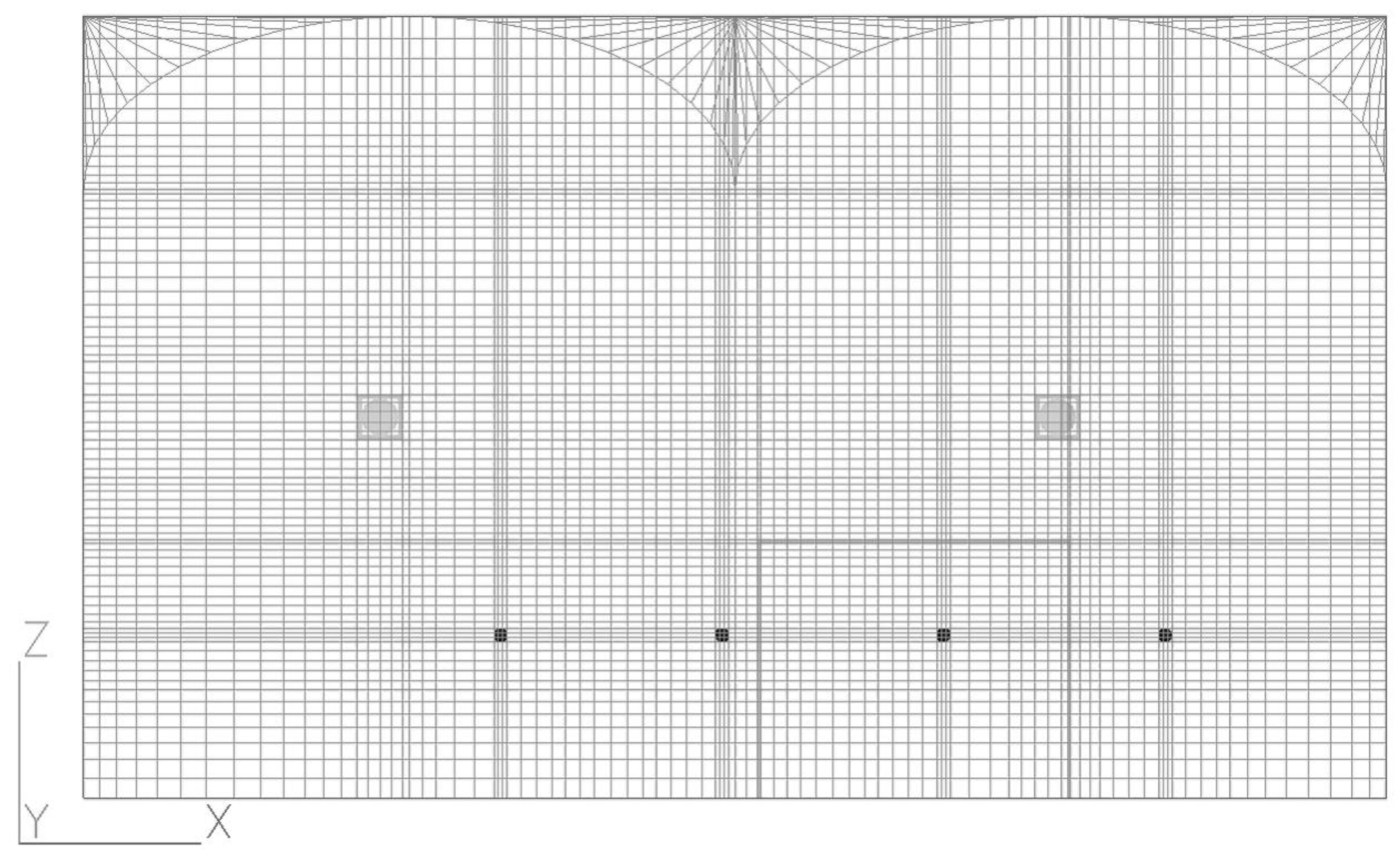
2.3.3. Greenhouse Model

The computational model greenhouse has dimensions of length 12 m, width 10 m, and height 6 m. The greenhouse model has four circulating fans, four shelves of cultivating bed for tomato, and four CO₂ perforated tubes on each shelf (Figure 6). Leakage paths were managed in the door area and for tiny gaps across the greenhouse rib structure between the wall and the roof [31].

Several turbulence models were tested to adopt suitable turbulence models in the greenhouse [5,32]. Natural ventilation of the greenhouse simulation was validated by different mesh sizes and different turbulence models to determine the accuracy of CFD simulation [20]. This study tested different turbulence models to simulate CO₂ distribution while considering CO₂ absorption by the photosynthesis process and found that the optimum convergence was achieved in the standard $k-\epsilon$ turbulence model. Accordingly, the standard $k-\epsilon$ turbulence model was applied in the greenhouse simulation.

2.3.4. Validation of the Greenhouse Model

The greenhouse simulation was conducted and compared with the measurement data of CO₂ enrichment. Model validation calculated the CO₂ distribution from CO₂ perforated tubes in the whole greenhouse. The number of meshes in the computational domain had 739,350 cells inside the greenhouse (Figure 7). The simulation model’s accuracy was assessed using RMSE and MAPE by comparing the percentage errors of each measured and simulated point.

Table 2. Computational conditions used for greenhouse model.

Parameter	Symbol	Unit	Value
Canopy photosynthesis rate	Pcg	g CO2 h−1 m−2ground area
CO2 density	Cc	g m−3	1839
Conductance of CO2	τc	m s−1	12.168 × 10−4
Crop respiration	R`	g h−1 m−2	2.84 × 10−2
Initial CO2	-	ppm	450
Leaf area density	$\mathrm{LAD}/\alpha$	m2leaf m−3row	0.67
Leaf area index	LAI	m2 m−2	1.1
The light use efficiency of the plant canopy	αc	g CO2 J−1	3.705 × 10−6
The incident light flux PAR	Jo	W m−2leaf	355

presents the computational conditions used for the three-dimensional CFD simulation.

Using a coefficient of variation (CV), the variability of CO₂ distribution inside the greenhouse was examined for two types of scenario cases, open and closed side ventilation and weather (rainy and sunny days). The 7070 points of CO₂ concentration were taken to measure the variability inside the greenhouse and 8484 points of CO₂ concentration for plants.

Note that the measurements of CO₂ concentration for chamber and greenhouse have been carried out at different date (4 August 2021, for CO₂ concentration measurement at chamber and 30 August 2021, for CO₂ concentration measurement at greenhouse that will be used for simulation cases). The data of LAI and some parameters that used in model were the data at the date of CO₂ measurement. Due to this, some parameters are different between the chamber and greenhouse.

3. Results and Discussion

3.1. Model Validation

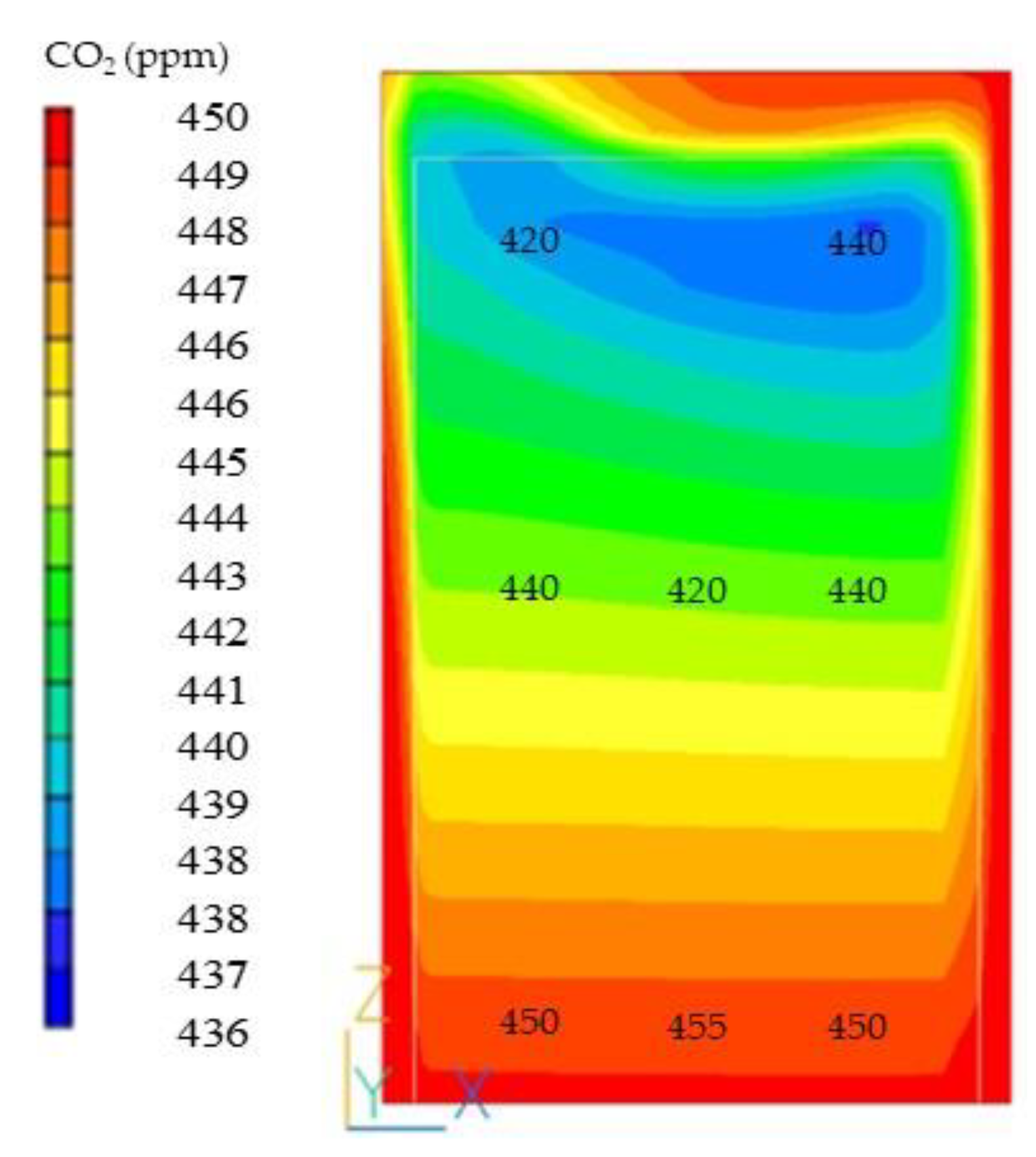
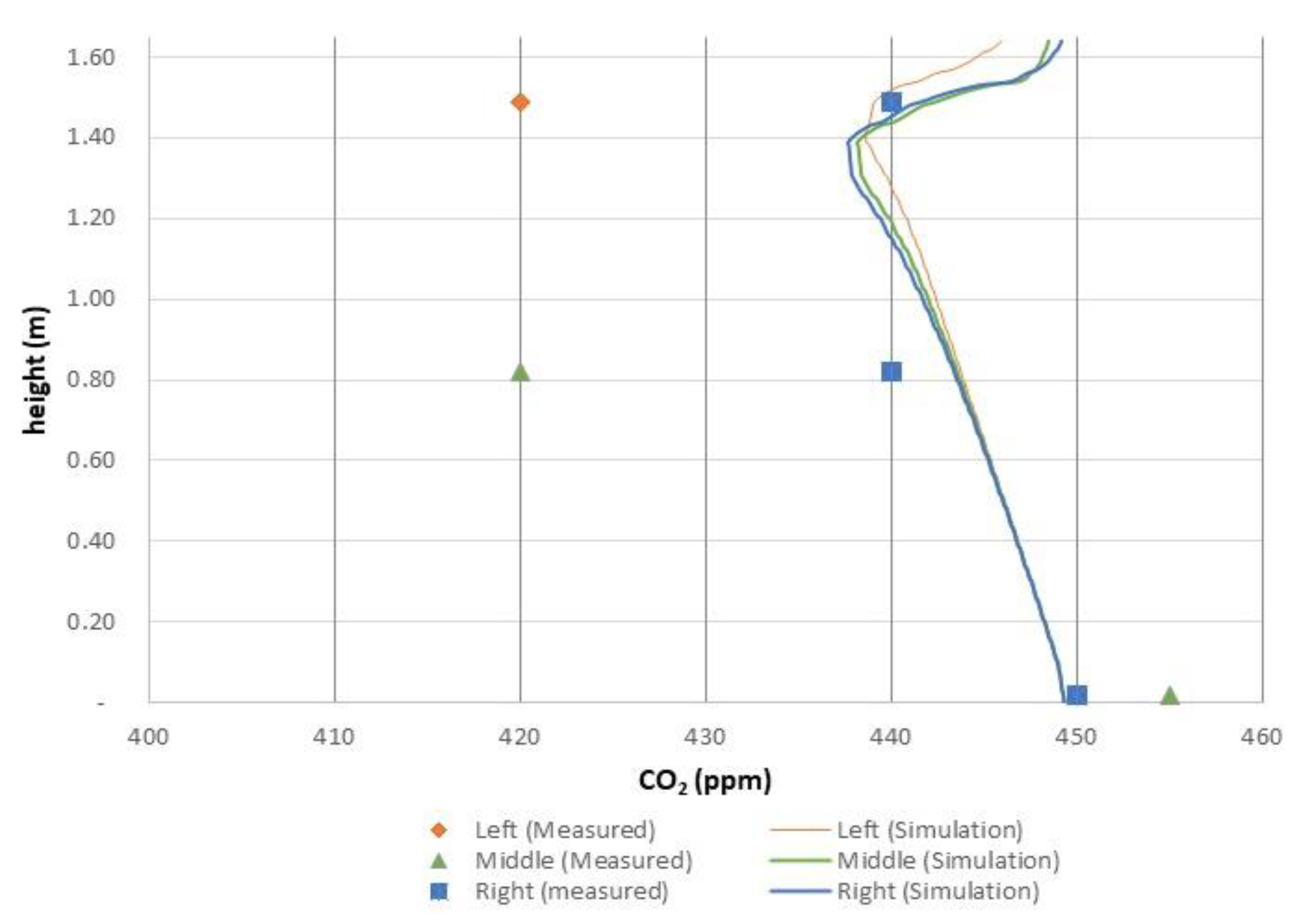
3.1.1. CO₂ Distribution Inside the Chamber

The measured CO₂ concentrations were compared with the simulated CO₂ distribution inside the chamber. Model simulation accuracy was evaluated by comparing each measured and simulated point’s percentage errors of

Table 3. Comparison of CO₂ concentration between measured and simulated data for model validation in the chamber.

Canopy Layer	Measured			Simulation			Percentage error (%)
	Left	Middle	Right	Left	Middle	Right	Left	Middle	Right
Top	420	─	440	439	442	442	4.53	─	0.36
Middle	440	420	440	444	443	443	0.84	5.59	0.76
Bottom	450	455	450	449	449	449	0.17	1.27	0.17
MAPE (%)	1.85	3.43	0.43
RMSE (ppm)	11.20	16.99	2.17

. The MAPE of the left, middle, and right parts of the chamber were 1.85%, 3.43%, and 0.43%, respectively, and the RMSE of left, middle, and right parts were 11.20, 16.99, and 2.17 ppm, respectively, according to the CFD model for CO₂ distribution.

The results showed that employing a tomato plant as a porous medium considered the photosynthetic process could reasonably predict CO₂ distribution. In comparison to the actual canopy of the tomato plant, the model tomato plant has been simpler. That is, the dense leaves were considered homogenous for the entire plant. Thus, the CO₂ concentration shows a decrease inside the porous medium (corresponding to tomato plant), where the air, including CO₂, may go through the canopy of the tomato plant; then, the CO₂ is absorbed by the process of photosynthesis (Figure 8).

The CO₂ concentration distribution according to the chamber measurement and simulation for each height were compared to evaluate numerical simulation properties (Figure 8 and Figure 9). These figures showed the simulation results of CO₂ concentration at the left and middle part were slightly overestimated. However, the simulation was still reasonable and can be used for greenhouse numerical simulation.

3.1.2. CO₂ Distribution Inside the Greenhouse

The greenhouse model validation was conducted according to the measurement data of Kumazaki, et al. [26], who studied influential positions of CO₂ supply in tomato plants inside the same greenhouse as the present study. In the present study, the simulation results were compared with the measurement data of CO₂ concentration in the condition 20 min after 1 h of CO₂ being supplied at the middle canopy (1.2 m above the ground, see Figure 10).

The CO₂ concentrations were measured at two sides of 3.4 m from the north and south wall with 0.6, 1.2, 1.8, 2.4, and 4.2 m above the ground. The initial simulation value of CO₂ concentration was assumed to be constant in every mesh inside the greenhouse, whereas the actual condition has various CO₂ concentrations. In contrast, model simulation accuracy was also evaluated by comparing the percentage errors of each measured and simulated point (

Table 4. Comparison of CO₂ concentration between measured and simulated data for model validation in greenhouse.

Height (m)	Measured (ppm)		Simulation (ppm)		Percentage Error (%)
	North	South	North	South	North	South
4.2	391	418	435	435	11.15	3.96
2.4	411	439	433	432	5.28	1.53
1.8	418	431	432	432	3.34	0.14
1.2	432	443	432	432	0.03	2.55
MAPE (%)	4.95	2.04
RMSE (ppm)	25.33	10.57

).

According to the results of the CO₂ distribution using the CFD model within the greenhouse, the MAPE of north and south were 4.95% and 2.04%, respectively, whereas the RMSE of north and south were 25.33 and 10.57 ppm, respectively, compared with the measured values. However, the simulation results in this study may be reasonable to predict the CO₂ distribution considering CO₂ absorption through the process of photosynthesis of the plant inside the greenhouse (Figure 11).

3.2. Simulation Cases for Greenhouse Model

Several simulations were conducted to analyze CO₂ distribution under the CO₂ enrichment described below. The cases were trial scenarios to determine the detailed CO₂ distribution while considering the photosynthesis process inside the greenhouse.

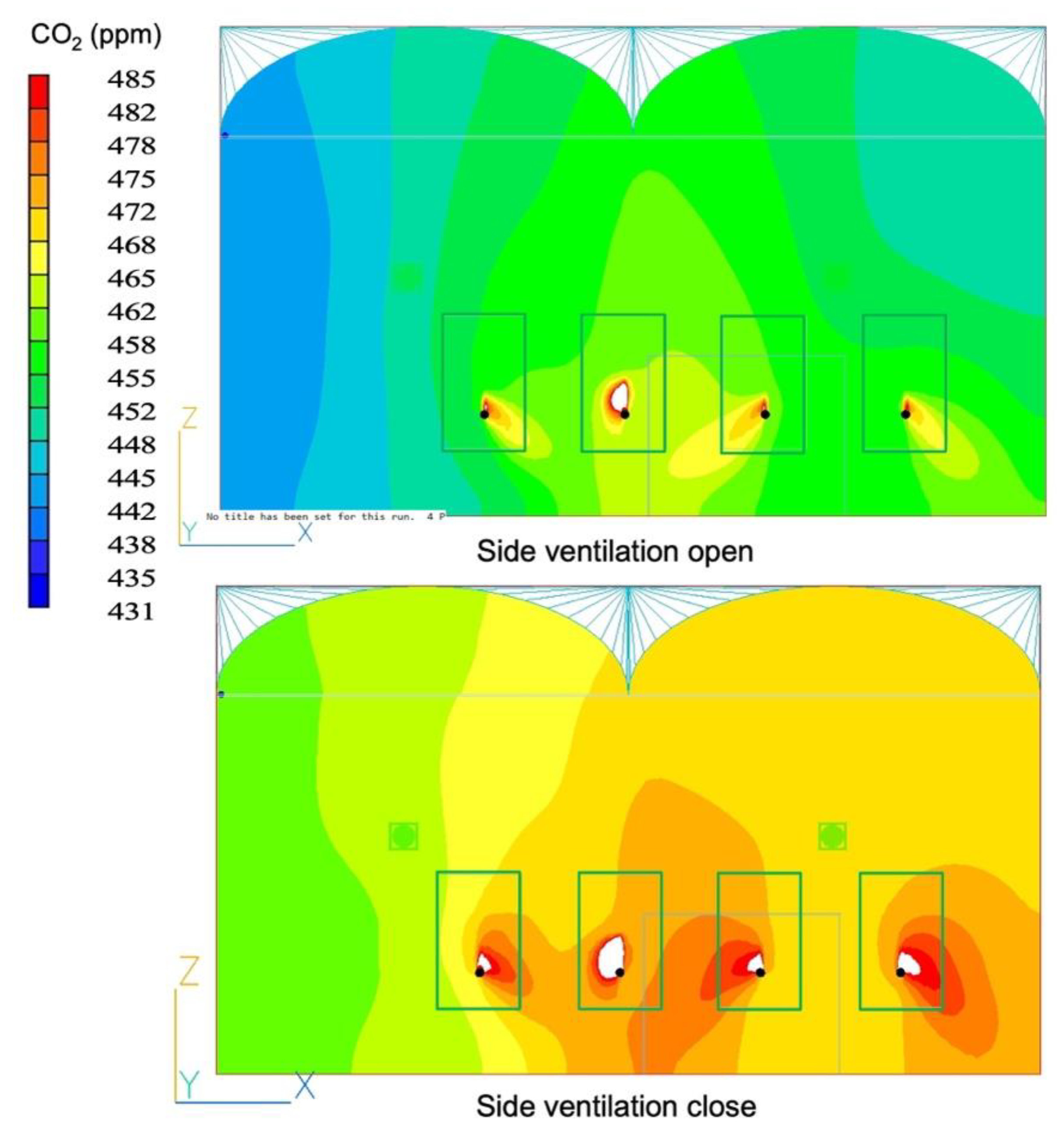
3.2.1. CO₂ Distribution toward Open and Closed Side Ventilation Inside the Greenhouse

Figure 11 shows the simulation of CO₂ distribution inside the greenhouse when 1160 ppm CO₂ concentration was supplied through perforated tubes inside the plants. The appearance of CO₂ emissions from the perforated tube was confirmed with the degradation colors inside of the plants. CO₂ distribution in case open and closed side vents were showed a slight difference in CO₂ concentration (Figure 12).

When the sidewall was opened (ventilated), the inflow wind from outside the greenhouse was continually updated to match the current wind velocity in each mesh [33]. The CO₂ concentration outside of the greenhouse (400 ppm) is lower than the initial CO₂ concentration inside the greenhouse (450 ppm), which may cause the CO₂ concentration near the ventilated wall to be lower. Furthermore, the position of the plants in the greenhouse was asymmetric (tend to the right side).

The effects of open side vents on CO₂ distribution were slightly significant, especially near the wall. In comparison to the case of open side vents, the case with closed side vents showed a slightly more uniform CO₂ concentration within the greenhouse. Although the side vents are closed, air circulators supported moving large volumes of air to provide even distribution. The quantitative evaluation of these results using CV shown in

Table 5. Coefficient of variations of CO₂ concentration in the case of side vents open and closed.

Parameter	Greenhouse		Plants
	Side Vent
	Open	Closed	Open	Closed
SD (ppm) 1	80	71	41	41
Mean (ppm)	438	457	464	476
CV (%) 2	18.2	15.6	8.8	8.7

¹ SD = Standard Deviation; ² CV = Coefficient of variation.

is 18.2% for the open and 15.6% for the closed side vents case for the whole greenhouse.

However, focusing on the variability of CO₂ concentration inside the plant, open (8.8%) and closed (8.7%) side vents produced essentially no substantial contribution to even the variation of CO₂ concentration in the plant canopy because no initial wind velocity was considered at both side vents in our case. Therefore, virtually no air exchange occurred between outside and inside the greenhouse.

Figure 12 (side ventilation open) showed the CO₂ concentration around the plant (rectangular shapes) was still maintained higher than ambient CO₂ concentration (approximately 400 ppm). This suggests that practical CO₂ enrichment was still effective even if side vent was open (in case, no outside wind).

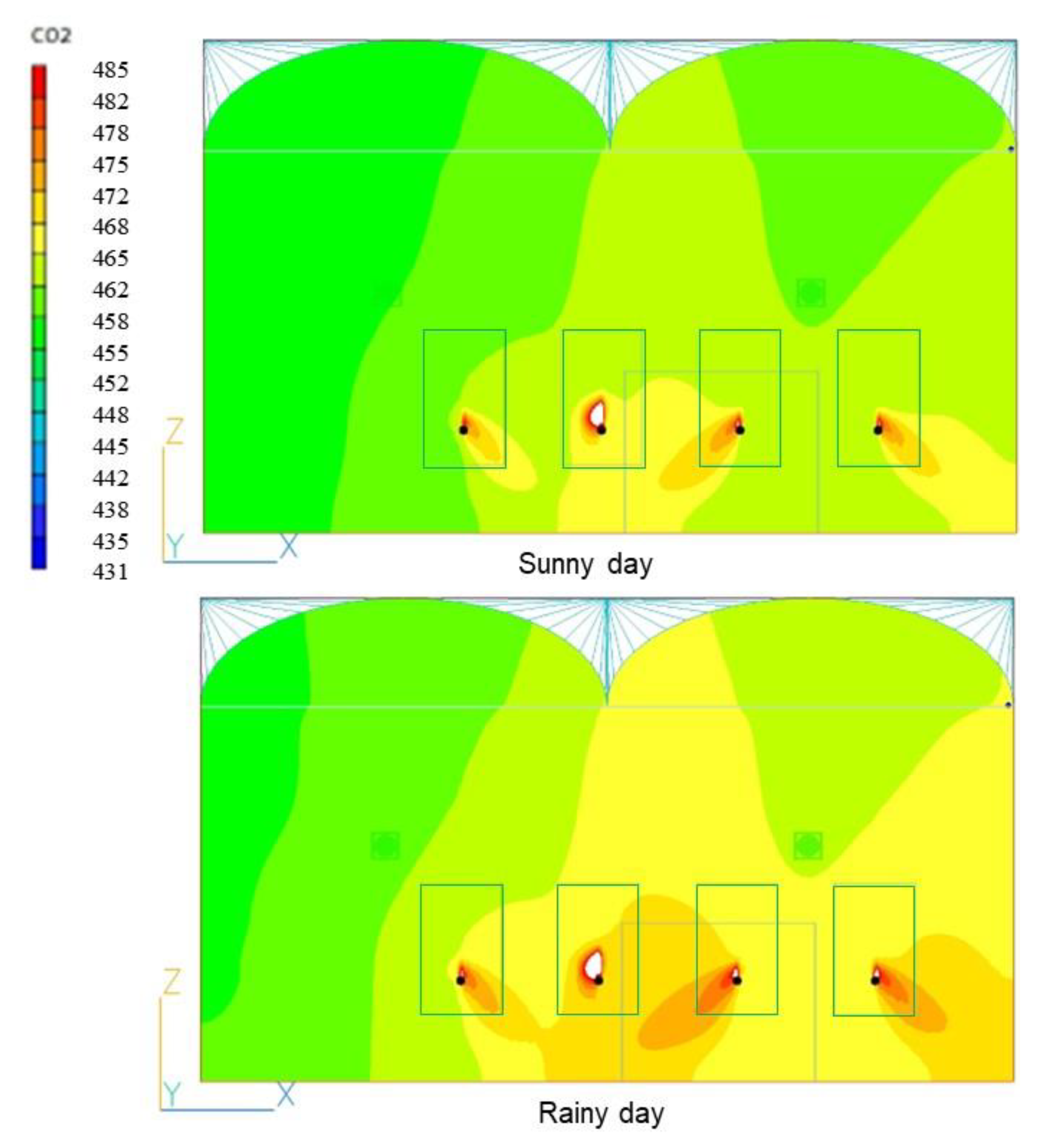
3.2.2. CO₂ Distribution toward on Sunny and Rainy Day Inside the Greenhouse

Simulations under treatment of 1000 ppm of CO₂ concentration, that had been done in the previous study [34,35] were conducted on a rainy day condition with PAR of 95 W m⁻² [36] and sunny day condition with PAR of 355 W m⁻² (based on NEDO solar radiation database).

There was a minor change in the CO₂ concentration between sunny and rainy days, according to the CO₂ distribution (Figure 13). The effects of solar radiation on CO₂ distribution were slightly significant. The case of rainy day showed a slightly more even of CO₂ distribution inside the greenhouse than the case of sunny day. For the entire greenhouse, the quantitative evaluation of these results using CV shown in

Table 6. Coefficient of variations of CO₂ concentration in the case of sunny and rainy day.

Parameter	Greenhouse		Plants
	Weather
	Sunny	Rainy	Sunny	Rainy
SD (ppm)	81	71	38	41
Mean (ppm)	446	457	467	476
CV (%)	18.1	15.6	8.1	8.7

is 18.1% for the sunny-day case and 15.6% for the rainy-day case. However, when it comes to the variability of CO₂ concentration inside the plant, sunny day (8.1%) and rainy day (8.7%) had essentially no effect on even the fluctuation of CO₂ concentration in the plant canopy.

Figure 14 shows the net photosynthesis estimations of the greenhouse model under treatment of 1000 ppm of CO₂ enrichment on a sunny and rainy day. The simulation results of a rainy and sunny days revealed the mean values of net photosynthesis (PCFD) of 3.82 and 9.69 µmol m⁻³ s⁻¹, respectively. The value of the net photosynthesis results seemed reasonable according to the study of Nederhoof and Vegter [29] and Xu et al. [37].

The PAR possibly compensated the CO₂ absorption through the photosynthesis process to be low at low light (rainy day) and was higher at high light (sunny day). Nevertheless, the different canopy layers such as the top layer (64%), middle layer (28%), and bottom layer (8%) were not assigned to the net photosynthesis as mentioned in the study by Reichrath et al. [38] because in this simulation the dense of leaves were assumed to be homogenous for the whole plant. Thus, the net photosynthesis results were almost constant for the entire plant. However, according to the simulation results, this model may be appropriate to estimate the net photosynthesis average.

The variability of CO₂ concentration inside the plant between a rainy and a sunny day determined practically no significant difference. Furthermore, these models revealed no significant connection PAR and even the variation in CO₂ content at the plants.

3.3. Discussion

The study presented numerically the details of CO₂ distribution inside the chamber and the greenhouse. The performance of model was validated by comparing measurement and simulation results obtained from CFD model considering photosynthesis model. The model reproduced the distribution of measured CO₂ concentration in the middle of plant, decreasing due to CO₂ absorption by photosynthesis. As proven by Molina-Aiz et al. [9], the CFD model could simulate photosynthesis accurately.

The chamber simulation results at the bottom of plant showed good agreement with the measurement results. The middle and upper left cross sections of the canopy showed that the simulation results were overestimated. This is likely due to the fact that the turbulence intensity near the fan located at the top of the chamber tends to be stronger than in other parts of the chamber, and thus the CO₂ concentration near the fan tends to be lower due to turbulent mixing.

Otherwise, turbulence at the right side of the chamber is small (laminar), and because the simulation adopted a laminar model, the simulation achieved a better agreement with measurement for right side of the chamber.

The greenhouse simulation results at the bottom of canopy showed good agreement with the measurement results. In position of 3.4 m from north wall showed simulation results were overestimated. The position of 3.4 m from the south wall showed simulation results that were slightly underestimated for heights of 1.2 and 2.4 m from the ground, while the results for heights of 1.8 and 4.2 m from the ground were overestimated.

This may be because the temperature condition was neglected in the simulation. As reported by Kim et al. [14] that unequal distribution of CO₂ depends on temperature and location. However, the simulation was still able to predict the detailed of CO₂ distribution considering CO₂ absorption at the plant by photosynthesis and the error values were still reasonable compared to previous study [9,11].

A few simulations of greenhouse were conducted to know the effect of various environmental conditions to the CO₂ distribution inside of the greenhouse. Cases with open and closed side vents showed that closed side vents have slightly more even of CO₂ concentration than those with open side vents inside the greenhouse. In contrast, the variability of CO₂ inside the plant, open (8.8%) and closed (8.7%) side vents, induced almost no significant improvement.

Additionally, cases of a rainy- and sunny-day model showed that photosynthetically active radiation possibly compensated CO₂ absorption through photosynthesis to be lower at low light (rainy day) and higher at high light (sunny day). Nonetheless, we found that there was almost no significant difference in the variation of CO₂ concentration in the plant between rainy and sunny days.

4. Conclusions

The distribution of CO₂ in the chamber and greenhouse was studied to understand the details of CO₂ concentration while considering the net photosynthesis. Consequently, the measurement and simulation values of the CO₂ concentration were well-validated. We determined that there would be no discernible difference in the CO₂ distribution between models with open and closed side vents of the greenhouse if there was no interference of air exchange for side vents. This study enables the prediction of net photosynthetic value concerning different PARs (rainy and sunny days).

The results showed that the average of net photosynthesis on a sunny day (9.69 µmol m⁻³ s⁻¹) was higher than on a rainy day (3.82 µmol m⁻³ s⁻¹). The link between the variability of CO2 concentration at the plants and the weather (sunny and rainy days), particularly PAR, did not appear to be significant. We determined that light and CO₂ distribution have an impact on the processes involved in photosynthesis. Thus, this research could take a role supporting agriculture technology.

In further research, an increase in the number of measurements would elucidate the CO₂ distribution considering photosynthesis. These could lead to a more accurate CFD model. Applying more parameters leads to simulation close to reality. To evaluate the photosynthetic model, consider the light distribution is based on the density of the canopy plant’s leaves. Therefore, expanding the experiments on greenhouse microclimate, which includes photosynthesis and transpiration in different crops in the greenhouse would be of importance.

References

1. Zhang, Y.; Kacira, M.; An, L. A CFD study on improving air flow uniformity in indoor plant factory system. Biosyst. Eng. 2016, 147, 193–205. [Google Scholar] [CrossRef]
2. Benni, S.; Tassinari, P.; Bonora, F.; Barbaresi, A.; Torreggiani, D. Efficacy of greenhouse natural ventilation: Environmental monitoring and CFD simulations of a study case. Energy Build. 2016, 125, 276–286. [Google Scholar] [CrossRef]
3. Santolini, E.; Pulvirenti, B.; Benni, S.; Barbaresi, L.; Torreggiani, D.; Tassinari, P. Numerical study of wind-driven natural ventilation in a greenhouse with screens. Comput. Electron. Agric. 2018, 149, 41–53. [Google Scholar] [CrossRef]
4. Roy, J.C.; Boulard, T.; Kittas, C.; Wang, S. Convective and ventilation transfers in greenhouses, part 1: The greenhouse considered as a perfectly stirred tank. Biosyst. Eng. 2002, 83, 1–20. [Google Scholar] [CrossRef] [Green Version]
5. Kim, R.W.; Lee, I.B.; Kwon, K.S. Evaluation of wind pressure acting on multi-span greenhouses using CFD technique, Part 1: Development of the CFD model. Biosyst. Eng. 2017, 164, 235–256. [Google Scholar] [CrossRef]
6. Kichah, A.; Bournet, P.E.; Migeon, C.; Boulard, T. Measurement and CFD simulation of microclimate characteristics and transpiration of an Impatiens pot plant crop in a greenhouse. Biosyst. Eng. 2012, 112, 22–34. [Google Scholar] [CrossRef]
7. Fang, H.; Li, K.; Wu, G.; Cheng, R.; Zhang, Y.; Yang, Q. A CFD analysis on improving lettuce canopy airflow distribution in a plant factory considering the crop resistance and LEDs heat dissipation. Biosyst. Eng. 2020, 200, 1–12. [Google Scholar] [CrossRef]
8. Roy, J.C.; Pouillard, J.B.; Boulard, T.; Fatnassi, H.; Grisey, A. Experimental and CFD results on the CO2 distribution in a semi closed greenhouse. Acta Hortic. 2014, 1037, 993–1000. [Google Scholar] [CrossRef]
9. Molina-Aiz, F.D.; Norton, T.; López, A.; Reyes-Rosas, A.; Moreno, M.A.; Marín, P.; Espinoza, K.; Valera, D.L. Using computational fluid dynamics to analyse the CO2 transfer in naturally ventilat0ed greenhouses. Acta Hortic. 2017, 1182, 283–292. [Google Scholar] [CrossRef]
10. Niam, A.G.; Muharam, T.R.; Widodo, S.; Solahudin, M.; Sucahyo, L. CFD simulation approach in determining air conditioners position in the mini plant factory for shallot seed production. In Proceedings of the 10th International Meeting of Advances in Thermofluids, Bali, Indonesia, 16–17 November 2018. [Google Scholar] [CrossRef]
11. Zhang, Y.; Yasutake, D.; Hidaka, K.; Kitano, M.; Okayasu, T. CFD analysis for evaluating and optimizing spatial distribution of CO2 concentration in a strawberry greenhouse under different CO2 enrichment methods. Comput. Electron. Agric. 2020, 179, 105811. [Google Scholar] [CrossRef]
12. Li, Y.; Ding, Y.; Li, D.; Miao, Z. Automatic carbon dioxide enrichment strategies in the greenhouse: A review. Biosyst. Eng. 2018, 171, 101–119. [Google Scholar] [CrossRef]
13. Kuroyanagi, T.; Yasuba, K.; Higashide, T.; Iwasaki, Y.; Takaichi, M. Efficiency of carbon dioxide enrichment in an unventilated greenhouse. Biosyst. Eng. 2014, 119, 58–68. [Google Scholar] [CrossRef]
14. Kim, C.H.; Kim, M.H.; Choi, E.G.; Jin, B.O.; Baek, G.Y.; Yoon, Y.C.; Kim, H.T. CO2 distribution due to thermal buoyancy in the greenhouse. In Proceedings of the 5th International Federation of Automatic Control on Biorobotics, Sakai, Japan, 27–29 March 2013. [Google Scholar] [CrossRef]
15. Shimomoto, K.; Takayama, K.; Takahashi, N.; Nishina, H.; Inaba, K.; Isoyama, Y.; Oh, S.C. Real-time monitoring of photosynthesis and transpiration of a fully-grown tomato plant in greenhouse. Environ. Control Biol. 2020, 58, 65–70. [Google Scholar] [CrossRef]
16. Campen, J.B. Greenhouse design applying CFD for Indonesian conditions. Acta Hortic. 2005, 691, 419–424. [Google Scholar] [CrossRef] [Green Version]
17. Wang, X.W.; Luo, J.Y.; Li, X.P. CFD based study of heterogeneous microclimate in a typical chinese greenhouse in central China. J. Integr. Agric. 2013, 12, 914–923. [Google Scholar] [CrossRef]
18. Boulard, T.; Roy, J.C.; Pouillard, J.B.; Fatnassi, H.; Grisey, A. Modelling of micrometeorology, canopy transpiration and photosynthesis in a closed greenhouse using computational fluid dynamics. Biosyst. Eng. 2017, 158, 110–133. [Google Scholar] [CrossRef]
19. Kuroyanagi, T. Prediction of leakage rate of a greenhouse using computational fluid dynamics. Acta Hortic. 2017, 1170, 87–94. [Google Scholar] [CrossRef]
20. Hong, S.W.; Exadaktylos, V.; Lee, I.B.; Amon, T.; Youssef, A.; Norton, T.; Berckmans, D. Validation of an open source CFD code to simulate natural ventilation for agricultural buildings. Comput. Electron. Agric. 2017, 138, 80–91. [Google Scholar] [CrossRef]
21. Saberian, A.; Sajadiye, S.M. The effect of dynamic solar heat load on the greenhouse microclimate using CFD simulation. Renew. Energy. 2019, 138, 722–737. [Google Scholar] [CrossRef]
22. Bouhoun, A.H.; Bournet, P.E.; Cannavo, P.; Chantoiseau, E. Development of a CFD crop submodel for simulating microclimate and transpiration of ornamental plants grown in a greenhouse under water restriction. Comput. Electron. Agric. 2018, 149, 26–40. [Google Scholar] [CrossRef]
23. Boulard, T.; Wang, S. Experimental and numerical studies on the heterogeneity of crop transpiration in a plastic tunnel. Comput. Electron. Agric. 2002, 34, 173–190. [Google Scholar] [CrossRef]
24. Majdoubi, H.; Boulard, T.; Fatnassi, H.; Bouirden, L. Airflow and microclimate patterns in a one-hectare Canary type greenhouse: An experimental and CFD assisted study. Agric. For. Meteorol. 2009, 149, 1050–1062. [Google Scholar] [CrossRef]
25. Zhang, Y.; Wei, Z.; Xu, J.; Wang, H.; Zhu, H.; Lv, H. Numerical simulation and application of micro-nano bubble releaser for irrigation. Mater. Express 2021, 11, 1007–1015. [Google Scholar] [CrossRef]
26. Kumazaki, T.; Ikeuchi, Y.; Tokairin, T. Relationship between positions of CO2 supply in a canopy of tomato grown by high-wire system and distribution of CO2 concentration in a greenhouse. Clim. Biosph. 2021, 21, 54–59. [Google Scholar] [CrossRef]
27. PHOENICS User Manual. The Mathematical Basis of PHOENICS. Available online: https://www.cham.co.uk/phoenics/d_polis/d_lecs/general/maths.htm (accessed on 18 February 2022).
28. Stathopoulou, O.I.; Assimakopoulos, V.D. Numerical study of the indoor environmental conditions of a large athletic hall using the CFD code PHOENICS. Environ. Model. Assess. 2008, 13, 449–458. [Google Scholar] [CrossRef]
29. Nederhoff, E.M.; Vegter, J.G. Canopy photosynthesis of tomato, cucumber, and sweet pepper in greenhouses: Measurements compared to models. Ann. Bot. 1994, 73, 421–427. [Google Scholar] [CrossRef]
30. Nurmalisa, M.; Tokairin, T.; Takayama, K.; Inoue, T. Numerical simulation of detailed airflow distribution in newly developed photosynthesis chamber. In Proceedings of the 2nd International Conference on Environment, Sustainability Issues, and Community Development (Virtual Conference), Semarang, Indonesia, 21 October 2020. [Google Scholar] [CrossRef]
31. Kuroyanagi, T. Investigating air leakage and wind pressure coefficients of single-span plastic greenhouses using computational fluid dynamics. Biosyst. Eng. 2017, 163, 15–27. [Google Scholar] [CrossRef]
32. Velázquez, J.F.; Gea, G.D.T.; Garcia, E.R.; Cruz, I.L.L.; Aguilar, A.R. Advances in Computational Fluid Dynamics Applied to the Greenhouse Environment. In Applied Computational Fluid Dynamics; Oh, H.W., Ed.; IntechOpen: London, UK, 2012; pp. 35–62. [Google Scholar] [CrossRef] [Green Version]
33. PHOENICS User Manual. VR Object Types and Attributes. Available online: https://www.cham.co.uk/phoenics/d_polis/d_docs/tr326/obj-type.htm (accessed on 20 February 2022).
34. Nederhoff, E.M.; Vegter, J.G. Photosynthesis of stands of tomato, cucumber, and sweet pepper measured in greenhouses under various CO2 concentrations. Ann. Bot. 1994, 73, 353–361. [Google Scholar] [CrossRef]
35. Kim, H.T.; Kim, C.H.; Choi, E.G.; Jin, B.O.; Yoon, Y.C.; Kim, H.T. The effect of thermal conditions on CO2 distribution in a greenhouse. Trop. Agric. Res. 2015, 26, 714. [Google Scholar] [CrossRef] [Green Version]
36. Romdhonah, Y.; Fujiuchi, N.; Shimomoto, K.; Takahashi, N.; Nishina, H.; Takayama, K. Averaging techniques in processing the high time-resolution photosynthesis data of cherry tomato plants for model development. Environ. Control Biol. 2021, 59, 107–115. [Google Scholar] [CrossRef]
37. Xu, S.; Zhu, X.; Li, C.; Ye, Q. Effects of CO2 enrichment on photosynthesis and growth in Gerbera jamesonii. Sci. Hortic. 2014, 177, 77–84. [Google Scholar] [CrossRef]
38. Reichrath, S.; Ferioli, F.; Davies, T.W. A simple computational fluid dynamics (CFD) model of a tomato glasshouse. Acta Hortic. 2000, 534, 197–202. [Google Scholar] [CrossRef]
Figure 1. Chamber inside the greenhouse.
Applsci 12 07756 g001
Figure 2. CO2 measurement points (•) at the front (left) and top (right)-view.
Applsci 12 07756 g002
Figure 3. The greenhouse for CO2 measurement.
Applsci 12 07756 g003
Figure 4. Chamber model: Fans are placed at the top left side of the chamber (▃ represents the fan). The rectangular shape inside of the chamber represent the plant.
Applsci 12 07756 g004
Figure 5. Meshing of chamber model: the dashed line square at top view represents fan ( Applsci 12 07756 i001). The rectangular shapes inside of the chamber represent the plants.
Applsci 12 07756 g005
Figure 6. Greenhouse model: (the squares represent fan circulator, rectangular shapes represent the plants, the circles represent CO2 perforated tube, and the thick lines and dots represent outlet).
Applsci 12 07756 g006
Figure 7. Meshing of greenhouse model: (the four rectangular shapes inside the chamber represent the plants, the circles represent CO2 perforated tube, and the squares represent fans).
Applsci 12 07756 g007
Figure 8. The CO2 distribution inside the chamber: The values are the measured data of the CO2 concentration.
Applsci 12 07756 g008
Figure 9. Measured and simulated data of CO2 concentration inside the chamber.
Applsci 12 07756 g009
Figure 10. CO2 concentration of measurement (north ♦ and south ▲) and simulation (north and south ─) data according to the position from the ground.
Applsci 12 07756 g010
Figure 11. CO2 distribution inside the greenhouse considering CO2 absorption through photosynthesis by plants (image taken at cross-section 3.4 m from south wall).
Applsci 12 07756 g011
Figure 12. The CO2 distribution inside of the greenhouse in case the side ventilations open and closed (image taken at cross-section 6 m from south wall).
Applsci 12 07756 g012
Figure 13. The CO2 distribution inside of the greenhouse in case the sunny and rainy day (image taken at cross-section 6 m from south wall).
Applsci 12 07756 g013
Figure 14. Net photosynthetic (PCFD) inside the greenhouse: 1000 ppm of CO2 enrichment cases on sunny and rainy day.
Applsci 12 07756 g014