Performance Optimization of Object Tracking Algorithms in OpenCV on GPUs

Abstract

Machine-learning-based computer vision is increasingly versatile and being leveraged by a wide range of smart devices. Due to the limited performance/energy budget of computing units in smart devices, the careful implementation of computer vision algorithms is critical. In this paper, we analyze the performance bottleneck of two well-known computer vision algorithms for object tracking: object detection and optical flow in the Open-source Computer Vision library (OpenCV). Based on our in-depth analysis of their implementation, we found the current implementation fails to utilize Open Computing Language (OpenCL) accelerators (e.g., GPUs). Based on the analysis, we propose several optimization strategies and apply them to the OpenCL implementation of object tracking algorithms. Our evaluation results demonstrate the performance of the object detection is improved by up to 86% and the performance of the optical flow by up to 10%. We believe our optimization strategies can be applied to other computer vision algorithms implemented in OpenCL.

1. Introduction

Computer vision is becoming essential to smart devices such as smartphones and self-driving cars [1,2]. Smart devices especially require well-performing object tracking techniques from computer vision [3,4]. Programs for object tracking convert images from input devices such as cameras into data that can be manipulated to recognize objects, calculate the movement, and track them. The Open Computer Vision library (OpenCV) [5] is a representative library supporting such image processing. OpenCV is open-source and supports various programming languages, including C/C++. Furthermore, OpenCV operates on a variety of platforms. Therefore, many applications adopt OpenCV to implement their computer vision applications [6,7,8,9].

Parallel computing devices are suited to processing images, such as the GPU, which can process large amounts of data in parallel. Thus, many studies have targeted utilizing the GPU to improve the performance of computer vision algorithms. OpenCV is also being developed to use GPGPU environments utilizing the open computing language (OpenCL) [10] framework or a vendor-specific computing platform [11], which can process data using parallel computing devices. Moreover, OpenCV 3.0 introduces a transparent API [12], in which the library itself runs appropriate parallel computing APIs according to available computing devices on a system. This alleviates the burden on application developers of explicitly selecting and manipulating parallel computing devices.

Although the OpenCV library is widely used in many applications because of its high portability, low computing power demands, and easy-to-use characteristics, its implementation has the performance potential to be further optimized on OpenCL GPU platforms. The library basically includes various well-known performance optimization techniques, such as local memory utilization, vectorization, and loop unrolling [13,14]. However, our profiling results showed that the application’s performance deteriorates owing to (1) failure to efficiently utilize GPU resources and (2) kernel call overhead when operating many kernels with short execution times sequentially.

This paper proposes techniques to improve the performance of object tracking algorithms in OpenCV. Especially, we focused on object detection and optical flow algorithms. Object detection is an important step to track objects [15,16,17]. However, using only object detection causes poor accuracy in tracking moving objects. Therefore, previous studies applied optical flow techniques to object detection for increasing the tracking accuracy of moving objects [1,2].

For the performance optimization, we analyzed two object detection algorithms and one optical flow algorithm. Based on the analysis, the paper presents two optimization techniques. The first is allowing the OpenCL kernel to maximize the device’s parallelism by optimizing GPU occupancy and adjusting the number of work-items. The second technique reduces the cost of OpenCL API calls and data transfers by avoiding unnecessary kernel calls.

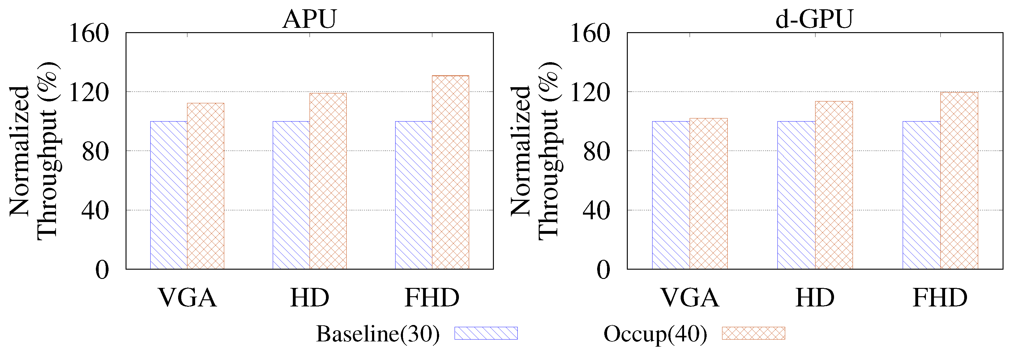
The proposed techniques were applied to two GPU computing environments: an accelerated processing unit (APU) in which the CPU and GPU share the main memory, and a discrete GPU, whose memory is separate from the CPU’s main memory. Our experiments show that the proposed optimization techniques improve the throughput of the object detection algorithms by up to 73% and 86% on the APU and the discrete GPU, respectively. In addition, our method to remove unnecessary kernel calls achieves 10% performance improvement.

Our contributions are as follows. First, we analyzed OpenCV’s object tracking algorithms running on parallel computing devices in terms of hardware level and investigated major factors affecting the algorithm’s performance. Next, we propose efficient schemes to better utilize the hardware resources of a parallel computing device for each object tracking algorithm: remapping variables, increasing global work size, and kernel merging. Finally, by applying the proposed schemes to OpenCV’s object tracking algorithms, we showed performance improvement per each scheme and analyzed them at the hardware usage level.

This paper is organized as follows. Section 2 describes the background, previous studies related to our work, and our motivation with the profiling results of the target algorithms. Then, in Section 3, we analyze the OpenCV object tracking algorithms: object detection with Haar/LBP classifiers and Farneback optical flow. Based on the analysis, Section 4 introduces optimization methods for object tracking algorithms in OpenCV. Section 5 demonstrates and analyzes the performance improvements gained by our optimization methods. Finally, Section 6 presents the conclusions of this paper with future work.

2. Background and Motivation

2.1. OpenCV and OpenCL

OpenCV [5] is a representative computer vision library developed by Intel. This library is open-source and used extensively in many companies and research groups. It implements various computer vision algorithms ranging from simple image filters to object tracking and a wide range of machine learning algorithms, from statistical ones to deep neural networks.

Processing images is more suitable for parallel computing devices such as GPUs because of its high data parallelism in computation. Hence, OpenCV has also developed to leverage GPGPU computing platforms, such as OpenCL [10] or vendor-specific platforms [11]. From OpenCV v3.0, the APIs in OpenCV are unified to transparently support available computing platforms (e.g., CPU, GPU, FPGA, etc.) on a system [12]. Hence, developers do not need to build multiple codes each specific to an accelerator, but can share a single code for various accelerators.

OpenCL [10,13] is a programming framework for efficiently exploiting computing accelerator platforms such as GPUs or FPGAs. OpenCL aims to produce applications independent of the execution platform. An OpenCL application consists of two types: a host program and kernel programs. On a CPU, a host program mainly preprocesses data for kernel programs. The host program checks device information in the platform, selects devices to run kernels, compiles kernel codes, and allocates memory space for kernels. The host program also commands computing devices to execute kernels or handles the data after kernels finish their operation [10].

The kernel program processes data on computing devices and operates through many threads in parallel. In OpenCL, a thread is referred to as a work-item, and a group of work-items is called a work-group. When running a kernel, the programmer allocates the number of work-items in an N-dimensional range called NDRange. NDRange is mapped to input or output data into one-, two-, or three-dimensional address spaces. Figure 1 shows an example of a work-item, a work-group, and NDRange. A local work size determines the number of work-items per work-group, and a global work size determines the total number of work-items in a workspace. Hence, the two values determine the number of work-groups in a workspace.

The OpenCL kernel can operate on various hardware, but each hardware can have different architectures, especially memory systems. Therefore, for the compatibility of the kernel program, OpenCL defines an abstract memory model, as shown on the left side of Figure 2. All work-items running on a computing device are accessible to global memory. In addition, data transferred from the host to the device are stored in global memory. A part of the global memory is dedicated to constant memory, which holds data that do not change, such as constant variables. Local memory is local to a work-group and is shared by work-items in a group. Local memory is generally faster than global memory in terms of latency and bandwidth. Each work-item has its private memory for its private values/variables. Private memory is usually backed by registers of computing units.

2.2. GPU Architecture

In this section, we explain a GPU architecture and then describe how OpenCL kernels and memory regions are mapped and executed on a GPU architecture. Although each vendor has its own implementation of GPUs, their high-level architecture is common. This section is based on a state-of-the-art GPU architecture for OpenCL execution [18]. The basic execution unit of GPU is a compute unit (CU). Generally, a high-performance GPU can process a huge amount of data with many CUs.

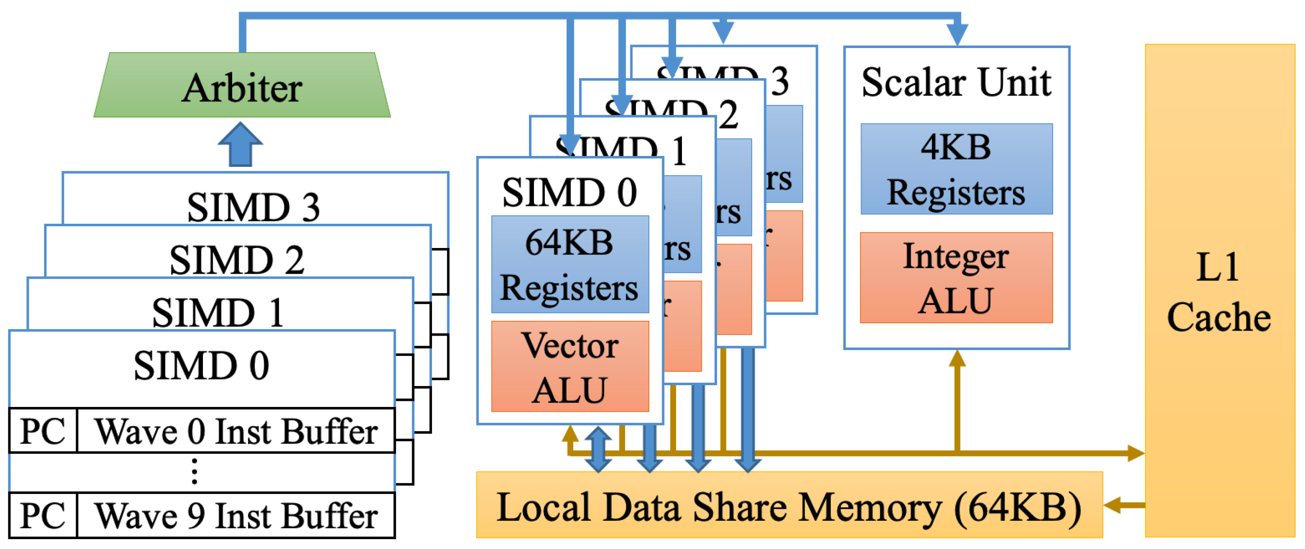
Figure 3 shows the architecture of a CU. A CU generally includes multiple single instruction, multiple data (SIMD) vector units, scalar units, local data share (LDS) memory, cache memory, texture units, and schedulers. For example, a CU in the GPUs used in this paper has four SIMD vector units, one scalar unit, and LDS memory. An SIMD unit consists of 16-lane vector arithmetic logic units (ALUs), and each lane is designed to compute four work-items. Thus, an SIMD unit can process 64 work-items, which is referred to as a wavefront. In addition, an SIMD unit has a buffer for ten wavefront instructions, as shown on the left side of Figure 3. The reason for this instruction buffer is to maximize the utilization of CUs. If data accessed by the work-item are not in memory, the work-item must wait until data are loaded to memory; this decreases the CU utilization. In this case, the execution of the next wavefront instruction can hide the latency derived from the memory load.

A CU can activate at most 40 wavefronts simultaneously because it has four SIMD units, and each unit has ten wavefront instruction buffers. Therefore, a GPU having eight CUs can process up to 320 wavefronts concurrently. Furthermore, since a wavefront handles 64 work-items, the GPU can compute up to 20,480 work-items simultaneously (320 wavefronts × 64 work-items per wavefront).

As described in Section 2.1, the abstract memory structure of OpenCL supports various computing devices. Figure 2 shows the correlation between the OpenCL memory abstraction and the GPU’s memory structure. In OpenCL, global and constant memories are accessible from all work-items, and these memories are mapped to the GPU memory (graphics double data rate (GDDR) memory of a discrete GPU or the system memory of an APU). Furthermore, local memory is local to work-items within the same work-group and is mapped to the GPU’s LDS memory, which is a fast memory private to each CU. Finally, private memory is mostly mapped to registers in a CU, but if registers are not enough to hold private memory, data on private memory can spill onto the GPU memory.

2.3. GPU Occupancy

Occupancy is one of the metrics to measure the GPU’s computing resource utilization. From the kernel’s perspective, resource utilization corresponds to the number of active wavefronts. Therefore, occupancy refers to the theoretical maximum percentage of wavefronts that can be activated simultaneously in a CU. As described in Section 2.2, each CU can execute 40 wavefronts simultaneously, and a 50% occupancy means 20 wavefronts are activated simultaneously in the CU. High occupancy generally shows high throughput in GPU computation since the more active wavefronts, the higher memory latency can be hidden, thereby reducing the stall cycles of SIMD units.

The occupancy can be limited when the kernel’s particular resource usage is large because the available resources are limited in a GPU. The following factors limit the occupancy:

–

The number of vector general purpose registers (VGPRs) and scalar general purpose registers (SGPRs) required by each work-item;

–

The work-group size (or the number of work-items in a work-group);

–

The amount of LDS memory used by each work-group.

An SIMD vector unit has a finite number of VGPRs (256 in our tested GPUs). This limits not only the number of VGPRs a wavefront (or a work-item) can use, but also the number of wavefronts that can be activated simultaneously in a CU [19]. The number of active wavefronts equals dividing the total number of VGPRs by the number of VGPRs used in a kernel [19]. For example, a kernel that uses 67 VGPRs can run with three (256/67) active wavefronts. At most 10 wavefronts can be active if each work-item (i.e., a kernel) uses no more than 25 VGPRs. If a kernel uses more than 128 VGPRs, only one wavefront can be active.

Table 1. The number of active wavefronts by VGPR usage in the kernel.

# of VGPR usages	<=24	25–28	29–32	33–36	37–40	41–48	49–64	65–84	85–127	128>=
Active waves	10	9	8	7	6	5	4	3	2	1

shows the number of active wavefronts by the usage number of VGPRs in the kernel, measured in our environment.

SGPRs can also limit the number of active wavefronts, but it hardly happens because the use of scalar values is not significant in typical image processing workloads. In our analysis, we found that SGPR was not a major contributor to limiting active wavefronts; this will be described in Section 2.4.

The number of active wavefronts is also limited by the size of a work-group. A CU can activate up to eight work-groups simultaneously [19]. The CU scheduler fetches wavefronts from the activated work-groups and schedules them to the SIMD vector units. Hence, if the size of a work-group is too small, a CU cannot activate the maximum number of wavefronts. For example, if one work-group is activated and the group has 256 work-items, each SIMD unit has only one active wavefront (64 work-items). Hence, the occupancy becomes only 10%. Hence, it is necessary to have a sufficient work-group size so that a CU can find a sufficient number of wavefronts to schedule.

The number of work-groups that can be activated is limited by the size of LDS memory usage per work-group. Whenever a work-group is activated in a CU, its local memory is allocated from the LDS memory. Hence, if the LDS memory is full, no more work-groups can be activated until a work-group completes. Therefore, the amount of local memory used by a work-group limits the number of activated work-groups in a CU. As mentioned above, the occupancy can be limited when a few work-groups are scheduled and each work-group has a few work-items. Hence, if LDS memory usage is high, only a few work-groups can be activated, thereby increasing the possibility of low occupancy.

2.4. GPU Profiler

The GPU profiler provides information for the occupancy. It also identifies factors restricting the occupancy by inspecting the resources such as registers and LDS memory. In general, because improving the performance of an application requires understanding its behavior, application profiling is required. Traditionally, profilers such as Linux perf [20] and gprof [21] have been used to improve the performance of applications. However, these profilers can only analyze operations running on the CPU. For this reason, GPU vendors provide the GPU profiler [22,23] to profile kernels. Those profilers can also leverage the hardware performance counter in the device to gather information while the kernel executes.

Table 2. Profiling results of the OpenCL kernel provided by the GPU profiler.

Variable	Value	Device Limit
Device Info
Device name	Carrizo
Number of compute units	8
Max number of waves per compute unit	40
Max number of work-groups per compute unit	40
Wavefront size	64
Kernel Info
Kernel name	runLBPClassifierStumpSimple
Vector GPR usage per work-item	67	256
Scalar GPR usage per work-item	94	102
LDS usage per work-group	0	65,536
Flattened work-group size	64	256
Flattened global work size	6144	16,777,216
Number of waves per work-group	1	4
Kernel Occupancy
Number of waves limited by vector GPR and work-group size	12	40
Number of waves limited by scalar GPR and work-group size	32	40
Number of waves limited by LDS and work-group size	40	40
Number of waves limited by work-group size	40	40
Limiting factor	VGPR
Estimated occupancy	30%

is a profiling result of the kernel provided by OpenCV by using a GPU profiler. The profiler provides three categories: device information, GPU kernel information, and kernel occupancy summary. The device information includes GPU hardware specifications such as the number of CUs and the maximum number of wavefronts per CU. In addition, information related to the kernel is provided. For example, the kernel’s hardware resource usage is identified, such as the VGPR usage per work-item and LDS memory usage per work-group. Lastly, the occupancy information is offered. Categories of number of waves limited by * indicate the number of wavefronts that are activated under the influence of the corresponding factor. Among them, the category of limiting factor(s) means factors affecting the kernel’s performance significantly. Estimated occupancy is given at the bottom of the profiling results. In Table 2, the kernel has 30% occupancy because only up to 12 of the 40 wavefronts are activated owing to the VGPR. As described in Section 2.3, no results showed the SGPR as a limiting factor.

2.5. Previous Studies on Optimizing GPU Kernels for Computer Vision Algorithms

Various studies have been presented to improve the throughput of computer vision algorithms, but most of them focused primarily on the algorithm itself. Borja et al. [24] utilized multidimensional scaling for optimizing object tracking algorithms. This work optimized the algorithms used for infrastructure and object positioning using multidimensional scaling at the software framework level. Favyen et al. [25] accelerated object tracking queries by adapting video frame rates. This work applied a hybrid machine learning model consisting of a convolutional neural network and a graph neural network to resolve the object tracking failure problem at low frame rates. The above studies modified the algorithm for object tracking optimization, so they have the advantage of being independent of the hardware. However, optimal performance may not be achieved in systems with scarce hardware resources due to no consideration of the hardware resource level.

Even for improving performance with accelerators such as a GPU, a major research topic is splitting and parallelizing the task of algorithms. Pramod et al. [4] presented a throughput optimization scheme for computer vision algorithms in embedded system environments and compared several hardware environments. Aby et al. [26] optimized the Viola–Jones algorithm used for face detection provided by OpenCV. This work targeted processing images on mobile platforms. Although those studies have the advantage of considering scarce hardware resource environments, they regarded only software optimization without profiling hardware utilization.

Moreover, most research applied well-known optimization methods to improve the GPU’s performance, such as leveraging local memory, loop unrolling, vectorization [3,27,28], etc. Hsiang-Wei et al. [3] optimized gesture recognition in OpenCV running on embedded heterogeneous multicore systems. However, the proposed techniques focused on optimizing the algorithm by applying such well-known optimization methods mentioned above without profiling hardware utilization.

The following are typical OpenCL kernel optimization techniques covered in previous studies.

• Leveraging local memory. OpenCL adopted an abstract memory model to support various types of devices. OpenCL memory is classified as global, local, constant, and private. Leveraging local memory can improve the performance of the OpenCL kernel because accessing local memory is faster than global memory [28]. Figure 4 is the gaussianBlur5 kernel function code in OpenCV. A __local indicator is required to use local memory in OpenCL, as shown in Line 6 in Figure 4. When an indicator is used in front of a variable, the variable is placed in local memory.
• Loop unrolling. Loop unrolling is a common optimization technique that copies the body statement of the loop multiple times. In general, loop unrolling improves performance by reducing executions of such instructions as incremental, comparative, and branch [30] and by exposing instruction-level parallelism if no loop-carried dependency exists. In OpenCL, all loop body statements can be re-written manually for loop unrolling. Furthermore, loop unrolling can simply apply by writing #pragma unroll in front of the loops, as shown in Lines 14 and 19 in Figure 4.
• Vectorization. The SIMD unit supports computations with a vector (an array of primitive data types, such as integer or float) [27]. Hence, by transforming an array of values into a vector, multiple values can be computed at once in parallel. In our target GPU architecture, an SIMD unit supports up to 16 integer/floating-point operations in parallel. To alleviate vectorization, sometimes, the structure of an array is transformed to make it more fit to the vector instructions [3].

3. Analysis of OpenCV Object Tracking Algorithms

Improving the application’s performance typically requires source code analysis and execution profiling. In this paper, we optimized two types of algorithms for object tracking in the OpenCV library. This section demonstrates an analysis of the two algorithms with a GPU profiler. The first is the object detection algorithm; it detects target objects in images. The second is the optical flow algorithm; it estimates the motion of objects using a series of images.

3.1. Object Detection Algorithm

For resource-constrained smart devices, object detection algorithms in OpenCV are an attractive solution. Although recent deep-neural-network-based object detection algorithms, such as YOLO [31], R-CNN [32], and SSD [33], show better performance in terms of accuracy, smart devices are not easily affording their high resource demands; for example, YOLO requires several gigabytes of GPU memory [34,35]. Therefore, in OpenCV, we target the two object detection algorithms, Haar [36] and local binary patterns (LBP) [37,38], whose resource demand is affordable in smart devices with pre-trained models.

3.1.1. Execution Flow

Object detection in OpenCV detects objects from images by utilizing information about the target objects. Its execution flow is shown in Figure 5a. The host program receives frames from video, images, and webcams to detect objects. To facilitate image detection, three functions, cvtColor, resize, and equalizeHist, preprocess the input frames. cvtColor converts the input frames into grayscale images. resize modifies the image size, and equalizeHist equalizes the histogram. It finally calls one of the two classifiers, Haar and LBP, which are the core algorithms of object detection.

Since OpenCV adopts transparent APIs [12], the host functions invoke the corresponding OpenCL kernels if the OpenCL platform is available on a system. The OpenCL kernels associated with the host functions are also depicted in the figure. Hence, cvtColor does not work on the CPU, but runs the RGB2Gray kernel on OpenCL computing devices. Furthermore, resize executes either the resizeLN or resizeSampler kernel. If the OpenCL sampler is available, it performs resizeSampler; otherwise, it performs resizeLN. equalizeHist calls multiple OpenCL kernels internally, but we omit detailed descriptions.

After the preprocessing, detectMultiScale finally calls the actual object detection algorithm. Using the Haar class launches the runHaarClassifier kernel, and using the LBP class executes the runLBPClassifierStumpSimple kernel. After the above process, the object detection result is obtained from the input image, such as size and coordinates.

3.1.2. Performance Analysis

Next, we analyze the performance of the object detection algorithm. We measured the latency of processing an image frame by varying the input video size from video graphics array (VGA) to full high definition (FHD). Since the Haar and LBP algorithms exhibit similar properties, we provide the results of the Haar algorithm only in this section. We used a human face training dataset available in OpenCV (haarcascade_frontalface_alt.xml). The experimental environment is described as APU in Section 5.1.

Figure 6a shows the frame processing time of object detection with the Haar algorithm with varying image resolution. In the figure, the frame processing time increases as video resolution increases because the data size increases. Figure 6b shows the breakdown of the frame processing time. As shown in the figure, the runHaarClassifier kernel accounts for most (60–80%) of the total execution time regardless of the resolution, while the other kernels occupy only 0.5–1.01%.

The results in Figure 6 show the following observations. First, as the resolution of images increases, the processing time increases rapidly, owing to the increased amount of data to process. Second, the runHaarClassifier kernel constitutes most of the execution time among the kernels at all resolutions. Therefore, to improve the performance of object detection using the Haar algorithm, optimizing the runHaarClassifier kernel is the most reasonable and effective approach.

3.1.3. Profiling Results

The GPU profiler offers a variety of features for analyzing OpenCL kernels, including an occupancy calculator and hardware performance counter.

Table 3. Profiling results of the runHaarClassifier kernel.

Occupancy Calculator	VGA	HD	FHD
Number of VGPRs used	76	76	76
Number of SGPRs used	94	94	94
LDS memory used	3840	3840	3840
Global work size	6144	6144	6144
Number of VGPR-limited waves	12	12	12
Number of LDS-limited waves	17	17	17
Kernel occupancy	30	30	30
HW Perf Counter	VGA	HD	FHD
GlobalWorkSize	768/8/1	768/8/1	768/8/1
WorkGroupSize	8/8/1	8/8/1	8/8/1
Time	18.44	66.59	154.42
LocalMemSize	3840	3840	3840
VGPRs	76	76	76
SGPRs	94	94	94
Wavefronts	96	96	96
FetchSize	37,467.44	149,170.43	414,024.81
CacheHit	76.99	70.93	66.39
VALUInsts	400,422.48	1,373,869.12	3,303,635.24
SALUInsts	78,081.27	262,919.63	626,184.05
VALUBusy	39.24	38.03	37.80
SALUBusy	6.77	6.49	6.35
MemUnitBusy	53.00	53.07	48.65
FlatVMemInsts	63,293.07	217,756.61	524,978.30

shows the profiling results of the runHaarClassifier kernel using the GPU profiler. As shown in the table, the number of VGPRs and SGPRs, the LDS memory, and the global work size do not change regardless of the image resolution. The two rows # of VGPR-limited waves and # of LDS-limited waves show the number of maximum wavefronts when each resource becomes the limiting factor. In particular, only 12 out of 40 wavefronts could be activated owing to being limited by the VGPR, which is shown in the row # of VGPR-limited waves. On the contrary, the LDS memory usage allows 17 active wavefronts, which is larger than that by the VGPR usage. Consequently, the VGPR usage of the kernel is the primary limiting factor to the wavefront activation, and the kernel occupancy is eventually 30% (12 over 40). In other words, reducing the VGPR usage can help increase the occupancy, thereby improving the performance of the kernel.

The GPU profiler can also utilize the hardware performance counter to collect the hardware information used by the kernel. Table 3 also shows the collected information during the execution of the runHaarClassifier kernel. In the table, the most directly impacting factors on the kernel performance are the Busy values (VALUBusy, SALUBusy, and MemUnitBusy); each value represents the utilization of the corresponding resources (i.e., vector ALU, scalar ALU, and GPU memory, respectively). Hence, high utilization indicates the kernel is being executed while effectively utilizing the hardware resources. However, the runHaarClassifier kernel shows low ALU utilizations, less than 40% for VALUBusy and 10% for SALUBusy. Furthermore, the MemUnitBusy is only about 50%. This is because the number of wavefronts is very low compared to the total available on the computing device. Although with 8 CUs, a total of 320 wavefronts are available (40 × 8 CUs), the actual number of active wavefronts is only 96 (12 wavefronts per CU) in Table 3.

To sum up, the resource utilization of the computing device deteriorates because excessive VGPR usage lowers the occupancy and the number of active wavefronts. Therefore, managing VGPR usage can improve the throughput of the object detection algorithm. Section 4.1 presents improvement techniques to resolve these issues.

3.2. Optical Flow Algorithm

Optical flow is a representative motion estimation algorithm, which compares two consecutive frames to calculate an object’s vector. The optical flow consists of sparse and dense optical flows. Sparse optical flow has high-speed throughput by minimizing computation only with interesting features. However, the sparse optical flow has poor accuracy due to exploiting only a fraction of points. Dense optical flow has high accuracy due to calculating all pixels, but a long computation time is its disadvantage. Therefore, optimizing the execution of dense optical flow algorithm achieves both high accuracy and suitable execution time.

Farneback optical flow [39] is a representative dense optical flow algorithm provided by OpenCV. Figure 5b shows the execution flow of the Farneback algorithm. The algorithm uses video files or cameras as the input media because it processes continuous images. At the preprocessing stage, the cvtColor function converts input images to grayscale images as in the Haar algorithm. After preprocessing, the calcOpticalFlowFarnback function calculates the optical flow vector. The calcOpticalFlowFarnback function launches diverse kernels to compute the optical flow, and these kernels are repeatedly executed in several groups. The gaussianBlur, resizeLN, and polynomiaExpansion kernels form one group, and updateMatrics, boxFilter5, and updateFlow form another. The execution flow of the entire calcOpticalFlowFarnback function contains both groups and repeats with the resizeLN and KF kernels.

The optical flow algorithm executes 77 kernels for processing two consecutive frames. The algorithm launches some kernels twice in succession because it processes continuous frames. In Figure 5b, the parts marked “×2” represent two consecutive kernel calls.

We measured and analyzed the performance of the Farneback optical flow algorithm. The experiment environment is identical to the Haar experiment case. Figure 7a shows the processing time of consecutive frames by resolution. As shown in the figure, the frame processing time increases when the video resolution increases. Figure 7b is the breakdown result of Figure 7a and represents the execution time proportion of each kernel. The parenthesis to the right of the kernel name means the number of launches while processing consecutive frames. For example, boxFilter5(12) means that the kernel boxFilter5 is called 12 times while processing consecutive frames. Therefore, a kernel that accounts for a large portion of the time may have a short execution time. Actually, the three kernels boxFilter, gaussianBlur, and updateMatrices account for a large portion in the frame processing time, but their unit execution time is not large (1–2% of the frame processing time). However, launching plenty of kernels can degrade the application’s performance because the OpenCL kernel launch involves additional costs such as data mapping and kernel queuing. Therefore, minimizing kernel call overhead is necessary to improve the algorithm’s throughput.

4. Performance Optimization of the OpenCV Object Tracking Algorithm

Based on the analysis in the previous section, we propose two optimization strategies. First, we improve the utilization of the GPU hardware by improving the parallelism of the OpenCL kernels. This strategy can be applied to the object detection algorithm since it shows low kernel occupancy, which is a major culprit of under-utilizing the parallelism of GPU hardware. Second, we propose to alleviate the frequent kernel call overheads of an OpenCL program. The frequent kernel calls not only incur the direct cost of kernel call overhead, but also waste unnecessary time to transfer data between consecutive kernels. This strategy is suitable for the optical flow algorithm. The following two subsections describe the two proposed optimization strategies, respectively.

Briefly, our performance optimization framework can be summarized as follows:

• When the VGPR usage is high and the LDS memory has free space, our optimization strategy is to remap variables from VGPRs to LDS memory (Section 4.1.1).
• When the number of generated active wavefronts is lower than the total capacity available in the GPU, our optimization strategy is to increase the number of wavefronts to fully utilize the SIMD (Section 4.1.2).
• When many kernel invocations are observed from the profiling results, our optimization strategy is to merge consecutive kernels that have an identical global/local work size into one merged kernel (Section 4.2).

4.1. Improving the Occupancy

The occupancy is the most effective metric for measuring the resource utilization of GPU hardware [19,40]. Therefore, increasing the occupancy generally leads to improving the kernel’s performance [40]. In particular, optimizing the kernel can significantly improve the application’s overall performance when a specific kernel accounts for a high execution time ratio. This section presents optimization schemes to increase the parallelism, thereby increasing the occupancy, of the kernels, which accounts for the largest fraction in the execution time of the object detection algorithm.

4.1.1. Mapping Data from the VGPR to LDS Memory

The VGPR usage is the most influential factor in limiting the occupancy. Even though the size of the work-group is large enough to supply a sufficient number of wavefronts, if the VGPR usage of the kernel is high, only a few wavefronts can be active. Hence, when LDS memory usage does not restrict the occupancy, variables can be moved from the VGPR to LDS memory to relieve the VGPR usage. However, mapping data from the VGPR to LDS memory can lead to occupancy degradation due to the LDS memory shortage. In addition, all work-items in a work-group share LDS memory data. Therefore, data selection to map to LDS memory must be carefully performed. We demonstrate the properties of variables that can and cannot be mapped to LDS memory by using the code in Figure 8.

LDS memory can contain variables that store the same data within the work-group because work-items in a work-group share LDS memory. This is the most effective approach to lowering the VGPR usage and not significantly expanding the LDS memory usage. If a variable is not the same across work-items, the variable movement from the VGPR to LDS requires a vector array, rather than a scalar variable in the LDS memory. For example, functions get_group_id() and get_global_size() return a value that is static and shared in a work-group. Therefore, variables storing the return values of them can be mapped to LDS memory, such as groupIdx and ngroups in Lines 10 and 11 in Figure 8.

In addition, LDS memory can include variables storing the same calculation results across all work-items. Two types of calculations correspond to returning the same result. The first is the calculation of a constant and a kernel function argument. The examples are the sumstep and invarea variables in Lines 10 and 17 in the figure. The second is the variable storing the result of calculation only among the arguments of the kernel function. The example is the normarea variable in Line 16. Furthermore, LDS memory can contain variables storing the result obtained by calculating between the above variables and non-private data of a work-item.

Work-item private data must be excluded from storing in LDS memory. For example, the lx and ly variables correspond to private data returned by the get_local_id() function in Lines 5 and 6 in the figure.

Table 4. Occupancy change of the runHaarClassifier kernel.

Variables Moved to LDS Memory	VGPR	Occupancy
Baseline	76	30
ngroups	59	40
sumstep	57	40
nofs0	51	40
normarea	58	40
invarea	58	40
nofs	55	40
ngroups, sumstep	57	40
ngroups, nofs0	51	40
ngroups, invarea	50	40
nofs0, nofs	47	50
ngroups, sumstep, nofs0, normarea, invarea, nofs	44	50

shows the runHaarClassifier kernel’s occupancy according to transferring variables from the VGPR to LDS memory. Baseline means the case without any variable movement. When only one variable is moved to LDS memory, the kernel uses 51 to 59 VGPRs (next five rows in the table). As shown in Table 1, the four wavefronts are active in this VGPR usage range. Because a CU provides ten wavefront buffers, the occupancy is 40% in this case. Furthermore, the table demonstrates that the more variables are moved to LDS memory, the less the VGPR usage becomes. The minimum VGPR usage is 44 when six variables are mapped to LDS memory (the bottom row). For 44 VGPR usage, the occupancy is 50%. Therefore, the runHaarClassifier kernel can achieve the maximum occupancy of 50% when moving the six variables from the VGPR to LDS memory. Moving two variables, nofs and nofs0, to LDS memory also acquires 50% of occupancy, as shown in the table (the row with boldface). Therefore, transferring only these two variables to LDS memory can achieve the maximum achievable occupancy while minimizing the increase in LDS memory usage. As described in Section 2.5, the variables are mapped to LDS memory by using the __local indicator front of the variables.

4.1.2. Securing Sufficient Wavefronts

As described in Section 2.2, an SIMD unit can handle 64 work-items, which is referred to as a wavefront. Since a CU has four SIMD units and each SIMD unit can concurrently execute ten wavefronts, a CU can theoretically activate up to 40 wavefronts simultaneously. The APU device, one of the environments used in this paper, has eight CUs. Therefore, the APU device can activate 320 wavefronts at the same time and process 20,480 work-items (320 × 64 work-items) simultaneously. This characteristic is important in achieving high occupancy because if the global work size is lower than 20,480 work-items, the GPU hardware has no more wavefronts to fill up all the wavefront buffers.

Most OpenCV computer vision algorithms perform parallel data operations to the individual pixel datum of the input images. Therefore, the input image size determines the number of kernel’s work-items. For example, 307,200 work-items can be created when a 640 × 480 VGA image is the input. Most OpenCV algorithms do not need to consider the number of work-items because many wavefronts are already active.

However, some kernels failed to activate all wavefronts provided by the GPU despite increasing the occupancy in Section 4.1.1; the runHaarClassifier kernel is an example of this case. As depicted in Section 3.1, the runHaarClassifier kernel generates only 96 active wavefronts. Although the input data size is large to process at once, the kernel configures a global work size (i.e., 6144 work-items) too small to utilize the total wavefronts supported by the GPU. Therefore, due to the necessity to generate more wavefronts in the kernels, we expand the global work size to 20,480 so that the runHaarClassifier kernel generates a total of 320 wavefronts. For this, we modified the fixed value assigned to the variable deciding the global work size. Note that when the global work size is set to generate more wavefronts, the algorithm’s performance will be improved more because the SIMD units are more utilized. However, when the global work size is set to generate more than 320 wavefronts, the performance will not be significantly improved. This is because instruction buffers in SIMD units are fully occupied, so increasing the global work size does not improve the algorithm’s parallelism.

4.2. Minimizing Kernel Call Overhead

An OpenCL program consists of host and kernel programs. A host program performs many preprocessing operations such as selecting computing devices, reserving a memory space, transferring data, and queuing kernels to execute. In addition, a host program must handle the output data after kernels finish their operations.

Computer vision algorithms generally process input images to produce output images, and such operations may consist of multiple consecutive operations. Subsequently, a series of computing operations is performed, and in this case, the output of a previous operation becomes the input of the next operation. When each operation is implemented as an individual kernel in the OpenCL framework, a host program needs to relay the output of a previous kernel to the input of the next one. This computing structure is natural and intuitive to a developer of a computer vision algorithm. Frequent kernel invocation, however, incurs high overheads, which are associated with OpenCL API calls, buffer allocation/management, and unnecessary data movement between kernels. As described in Section 3.2, the Farneback optical flow algorithm is such a case, launching many kernels.

Kernel merging is an effective method to alleviate such overheads. If adjacent kernels share data and have no data dependency between work-items, they can be unified into one kernel. Consequently, the overheads associated with kernel invocation, such as buffer allocation and data transfer, can be eliminated. Figure 9 shows the flowchart of our kernel merging algorithm. This algorithm merges kernels if consecutive kernels have data dependency with each other and identical global/local work sizes.

Table 5. Work size information for Farneback optical flow kernels.

Kernel Name	Global Work Size	Local Work Size	Kernel Merge
gaussianBlur	768/480/1	256/1/1
resizeLN	256/64/1	NULL
polynomiaExpansion	256/60/1	256/1/1
gaussianBlur	768/480/1	256/1/1
resizeLN	256/64/1	NULL
polynomiaExpansion	256/60/1	256/1/1
updateMatrices	96/64/1	32/8/1
boxFilter5	256/60/1	256/1/1
updateFlow	96/64/1	32/8/1	updateFM
updateMatrices	96/64/1	32/8/1
boxFilter5	256/60/1	256/1/1
updateFlow	96/64/1	32/8/1	updateFM
updateMatrices	96/64/1	32/8/1
boxFilter5	256/60/1	256/1/1
updateFlow	96/64/1	32/8/1
resizeLN	256/120/1	NULL
resizeLN	256/120/1	NULL
KF	256/120/1	NULL	resizeLN
KF	256/120/1	NULL

shows the kernels in the main loop of the Farneback algorithm shown in Figure 5b. The table includes the kernel names and their global and local work sizes. In the table, four kernels are candidates of kernel merging: updateFlow, updateMatrices, resizeLN, and KF. These kernels are executed in a row, have identical global and local work sizes, and transfer data from a previous kernel to the next. Therefore, we modified the resizeLN and KF kernels so that the resizeLN kernel executes the operation of the KF kernel. Please note that the two pairs of the two kernels process two different (consecutive) frames. Hence, merging the two kernels does not affect the result of the algorithm. Furthermore, we introduced a new updateFM by merging the two kernels, updateFlow and updateMatrices. The kernel after the kernel merging is shown in the table as well.

5. Evaluation

5.1. Environment

In this section, we evaluate the performance impact of our optimizations.

Table 6. Experiment environment configuration.

Hardware		APU	Discrete GPU (d-GPU)
CPU		RISC CPU 3.4 GHz	CISC CPU 3.5 GHz
	Core Frequency	800 MHz	1000 MHz
GPU	Number of CUs	8	28
	Number of PEs	512	1792

summarizes our experiment environments. We used two hardware environments. The first environment is an APU heterogeneous system (denoted as APU) on which a CPU and GPU share the main memory. The second system is a discrete GPU system (denoted as d-GPU) on which a GPU has its private memory separated from the main memory. The detailed specification of the system, as well as the GPU configuration can be found on the table. The software environments are Ubuntu version 14.04, OpenCV version 3.1, and OpenCL version 2.0 for the two hardware environments.

We applied the optimization schemes presented in Section 4 to the object recognition algorithms analyzed in Section 3. The baseline of each scheme is denoted as baseline, which indicates the original implementation of each algorithm. The proposed optimization techniques are denoted as follows:

• occup: The occupancy increase technique by moving variables from the VGPR to LDS memory (Section 4.1.1).
• wave: The occupancy increase technique by increasing the global work size to secure a sufficient number of active wavefronts (Section 4.1.2).
• merge: The optimization technique that merges kernels with identical global work sizes to reduce kernel call overheads (Section 4.2).

5.2. Experimental Results

5.2.1. Object Detection with the Haar Classifier

In this algorithm, the runHaarClassifier kernel occupied the largest portion in the execution time as described in Section 3.1. Therefore, optimizing the kernel can be the most effective optimization to improve the performance of the object detection algorithm. Our analysis in Section 3.1 revealed that the algorithm has low occupancy, thereby under-utilizing the GPU. Therefore, we applied the two optimization schemes, occup and wave, to increase the number of active wavefronts.

As compared to the baseline, occup improved the average throughput by 37% and 47% in the APU and d-GPU environments, respectively. Wave improved the average throughput by 44% and 34% over the baseline in the APU and d-GPU environments, respectively. Furthermore, occup and wave can be combined together, which is denoted as occup + wave. As compared to the baseline, occup + wave improved the throughput further by 67% and 77% in the APU and d-GPU environments, respectively.

Table 7. Hardware performance counter results of runHaarClassifier.

	Baseline	Occup	Wave	Occup + Wave
GlobalWorkSize	768/8/1	768/8/1	2560/8/1	2560/8/1
WorkGroupSize	8/8/1	8/8/1	8/8/1	8/8/1
Time	154.42	109.40	102.88	89.15
LocalMemSize	3840	3840	3840	3840
VGPRs	76	47	76	47
Wavefronts	96	96	320	320
FetchSize	414,025	423,297	415,139	432,954
VALUInsts	3,303,635	2,774,580	991,668	832,949
SALUInsts	626,184	626,184	188,395	188,395
LDSInsts	389,382	390,784	116,815	117,238
VALUBusy	37.80	38.28	54.38	49.40
SALUBusy	6.35	8.11	9.15	10.58
MemUnitBusy	48.65	68.51	66.29	74.04
FlatVMemInsts	524,978	526,380	157,493	157,917

shows the profiling result of the runHaarClassifier kernel with FHD using a hardware performance counter. The table demonstrates which factors in the GPU improve the kernel’s performance. In the table, VALUInsts, SALUInsts, and FlatVMemInsts indicate how many instructions are executed per work-item in VALU, SALU, and LDS memory. Furthermore, the VALUBusy, SALUBusy, and MemUnitBusy values indicate the time ratio that the unit is active while the kernel executes.

Figure 10 shows the throughput of the runHaarClassifier kernel in the object detection algorithm. The results in the figure are normalized to the baseline. The number in parentheses is an actual occupancy while running on real GPU hardware; baseline(30) indicates that the baseline showed 30% of the actual occupancy.

The value of VALUInsts for occup was significantly lower than that of the baseline. This result is because more work-items were simultaneously activated by our scheme, improving the occupancy. Furthermore, a significant increment of the MemUnitBusy value suggests that the accessing memory unit was pipelined more efficiently than before. In other words, memory access per unit time increased because more work-items were concurrently activated.

Experimental results in Wave also show a significant reduction of VALUInsts, SALUInsts, and FlatVMemInsts due to the increasing number of generated work-items. In addition, the VALUBusy and SALUBusy values increased because the Wave case activates the total number of wavefronts provided by the GPU, unlike activating the few wavefronts in the occup case.

5.2.2. Object Detection with the LBP Classifier

The runLBPClassifierStumpSimple kernel accounts for most of the LBP algorithm’s execution time. Its occupancy is 30%, and the VGPR usage is the main occupancy limiting factor. Unlike the Haar algorithm, the LBP algorithm produces 384 wavefronts on the APU environment, which means that the global work size is large enough to supply sufficient work-items, as well as wavefronts. Accordingly, wave did not need to be applied because the algorithm activates more than 320 wavefronts. Therefore, we applied only occup to the object detection with the LBP algorithm.

Figure 11 shows the throughput of the LBP object detection algorithm. With occup, mapping data from VGPR to LDS memory improved the occupancy by 30% to 40%. Therefore, the performance of the algorithm was improved by up to 31% and 21% in the APU and d-GPU environments as compared to the baseline.

Table 8. Hardware performance counter results of runLBPClassifierStumpSimple.

	Baseline	Occup
GlobalWorkSize	1536/16/1	1536/16/1
WorkGroupSize	16/16/1	16/16/1
Time	32.20	26.76
LocalMemSize	0	128
VGPRs	67	64
Wavefronts	384	384
FetchSize	80,516.25	110,256.56
VALUInsts	374,354.74	329,929.70
SALUInsts	17,289.77	15,461.60
LDSInsts	0	203.53
VALUBusy	75.78	79.89
SALUBusy	3.26	3.48
MemUnitBusy	91.31	91.06
FlatVMemInsts	36,950	32,672

summarizes the measurements of the hardware performance counters while running the runLBPClassifierStumpSimple kernel. The baseline showed 30% of occupancy due to 67 VGPR usage, but occup achieved 40% occupancy by reducing its VGPR usage to 64. Significant differences in the activation ratio of the ALU and memory units did not appear between baseline and occup because the original activation ratio in the baseline is already high. However, both the VALUBusy and VALUInsts values demonstrate that the performance was improved because of the increased active work-items by achieving higher occupancy.

5.2.3. Farneback Optical Flow

The Farneback optical flow algorithm showed its performance overhead from launching many kernels. Therefore, the kernel merge technique can improve the Farneback algorithm’s overhead. Section 4.2 dealt with the kernel merge technique and described candidate kernels in the Farneback algorithm for merging.

Figure 12 shows the performance improvement of the optical flow algorithm after applying the kernel merge technique. Please note that the operation of the kernel KF is absorbed into the kernel resizeLN, and two kernels updateFlow and updateMatrics are merged into a new kernel updateFM. As described in Section 4.2, decreasing the cost of API calls and data transfer causes performance improvement. The kernel merge scheme achieved average performance improvement with 10% and 6–8% in the APU and d-GPU environments as compared to the baseline.

The analysis of the OpenCL API calls and the kernels of the Farneback algorithm can identify factors leading to performance improvement.

Table 9. The execution time of OpenCL APIs with Farneback optical flow.

API Name	Baseline (ms)	Merge (ms)
clEnqueueMapBuffer	2234.95	2116.45
clEnqueueWriteBuffer	1907.73	1827.59
clReleaseMemObject	699.57	719.62
clEnqueueNDRangeKernel	254.17	237.53
clEnqueueReadBuffer	128.10	125.74
clFinish	27.02	14.94
clSetEventCallback	13.33	11.21
clSetKernelArg	12.65	12.76
clCreateKernel	11.14	10.73
clEnqueueUnmapMemObject	6.69	6.48
clCreateBuffer	5.58	5.71
clReleaseEvent	1.89	1.80
clReleaseKernel	1.78	1.69
clGetDeviceInfo	1.75	2.17
Total	5306.34	5094.41

shows the profiling results of the OpenCL API calls while running the Farneback optical flow algorithm. The table includes the execution time of each API. The total execution time of API calls is reduced by 210 ms from the baseline. Most of the execution time reduction came from APIs related to the buffer memory. By merging two consecutive kernels, the overheads associated with data transfer from one to the next can be saved. Hence, it is unnecessary to allocate a buffer, establish address mapping, and read/write from/to a buffer, so the overheads can be eliminated between the two kernels.

Table 10. The number of calls and execution time of the kernels of Farneback optical flow.

	# of Calls		Execution Time (ms)
Kernel Name	Baseline	Merge	Baseline	Merge
boxFilter5	1092	1092	1515.54	1504.72
gaussianBlur	728	728	1022.40	1020.15
polynomialExpansion	728	728	253.71	252.71
split	90	90	49.77	49.86
merge	91	91	46.99	47.27
convertTo	182	182	31.49	31.50
RGB2Gray	92	92	16.28	16.23
set	182	182	1.06	1.06
updateFlow	1092	364	352.79	120.08
updateMatrices	1092	364	1023.37	340.51
updateFM	0	728	0.00	800.23
resizeLN	1274	1274	154.98	154.72
KF	546	0	59.25	0.00
Total	7189	5915	4527.61	4339.03

shows the execution time and the number of kernel calls before and after applying the kernel merge technique. The table includes the number of calls and the total execution time of the kernels of the algorithm. First, the number of calls and the execution time of KF are eliminated because the kernel operation is merged into resizeLN. Second, two third of the execution of the two kernels updateFlow and updateMatrices are replaced to the unified kernel updateFM. Accordingly, merge saved the time to invoke the kernels and the buffer management overhead associated with the kernels.

5.3. Discussion

Our schemes improved the performance of the object tracking algorithms through the following methods. First, hardware utilization and algorithm performance were improved through the remapping of variables to another hardware resource. Next, the algorithm’s performance was improved by configuring the global work size based on the number of work-items available in the hardware. Finally, the algorithm’s performance was improved by eliminating preprocessing in the host program, which is redundant for GPU kernel launch.

Those results can provide insights to the computer vision community as follows. First, the algorithm’s performance can be improved without optimizing the algorithm’s flow or supplying hardware resources. For this, we propose three schemes: distribution of hardware usage by remapping variables, maximizing computing resource utilization by increasing global work size, and reducing the host’s computing time by kernel merging for minimizing the parallel computing device’s idle time. Next, all of the above schemes can be automated. For example, variable remapping is already a common technique in the compiler community [42,43], and kernel merging can be performed through work size detection at the compiler level. Furthermore, fixing the global work size is possible through the information of parallel computing devices. Optimizing object tracking algorithms automatically through device and kernel profiling is our future work.

6. Conclusions

This paper proposed the optimization techniques for the object tracking algorithms in the OpenCV library. We targeted two object tracking algorithms, object detection with the Haar/LBP classifier and Farneback optical flow, which are affordable solutions to resource-constrained computing systems, such as smart devices. Based on careful profiling of the algorithms implemented in the OpenCV library, we proposed and applied various optimization techniques. The evaluation results demonstrated that the proposed optimization techniques successfully improved the performance (throughput) of the object tracking algorithms.

The constraint of our research is that programmers should manually locate the algorithm’s performance bottleneck and apply an appropriate optimization scheme. This may undermine the advantage of OpenCV’s transparent API introduced for the programmer’s convenience. Therefore, our future work is developing a profiler that automatically profiles OpenCV/OpenCL applications and applies such optimization strategies to them.

References

1. Gao, P.; Sun, X.; Wang, W. Moving object detection based on kirsch operator combined with Optical Flow. In Proceedings of the 2010 International Conference on Image Analysis and Signal Processing, Zhejiang, China, 9–11 April 2010; pp. 620–624. [Google Scholar]
2. Cho, J.; Jung, Y.; Kim, D.S.; Lee, S.; Jung, Y. Moving object detection based on optical flow estimation and a Gaussian mixture model for advanced driver assistance systems. Sensors 2019, 19, 3217. [Google Scholar] [CrossRef] [PubMed] [Green Version]
3. Sung, H.W.; Chang, Y.M.; Wang, S.C.; Lee, J.K. OpenCV Optimization on Heterogeneous Multi-core Systems for Gesture Recognition Applications. In Proceedings of the 2016 45th International Conference on Parallel Processing Workshops (ICPPW), Philadelphia, PA, USA, 16–19 August 2016; pp. 59–65. [Google Scholar]
4. Poudel, P.; Shirvaikar, M. Optimization of computer vision algorithms for real time platforms. In Proceedings of the 2010 42nd Southeastern Symposium on System Theory (SSST), Tyler, TX, USA, 7–9 March 2010; pp. 51–55. [Google Scholar]
5. Open Source Computer Vision Library. 2015. Available online: http://docs.opencv.org/3.1.0/ (accessed on 2 July 2022).
6. Li, S.; Wu, J.; Long, C.; Lin, Y.B. A full-process optimization-based background subtraction for moving object detection on general-purpose embedded devices. IEEE Trans. Consum. Electron. 2021, 67, 129–140. [Google Scholar] [CrossRef]
7. Battaglia, F.; Iannizzotto, G.; La Rosa, F. An open and portable software development kit for handheld devices with proprietary operating systems. IEEE Trans. Consum. Electron. 2009, 55, 2436–2444. [Google Scholar] [CrossRef]
8. Chai, Y.; Shin, S.; Chang, K.; Kim, T. Real-time user interface using particle filter with integral histogram. IEEE Trans. Consum. Electron. 2010, 56, 510–515. [Google Scholar] [CrossRef]
9. Chun, J.B.; Jung, H.; Kyung, C.M. Suppressing rolling-shutter distortion of CMOS image sensors by motion vector detection. IEEE Trans. Consum. Electron. 2008, 54, 1479–1487. [Google Scholar] [CrossRef]
10. Khronos. OpenCL Reference Pages. 2013. Available online: https://www.khronos.org/registry/cl/sdk/2.0/docs/man/xhtml/ (accessed on 2 July 2022).
11. NVIDIA. CUDA Programming Guide v7.5. 2016. Available online: http://docs.nvidia.com/cuda/cuda-c-programming-guide/index.html (accessed on 2 July 2022).
12. OpenCV 3.0. Available online: https://opencv.org/opencv-3-0/ (accessed on 2 July 2022).
13. Munshi, A.; Gaster, B.; Mattson, T.G.; Ginsburg, D. OpenCL Programming Guide; Pearson Education: London, UK, 2011. [Google Scholar]
14. Guide, D. Cuda c programming guide. NVIDIA 2013, 29, 31. [Google Scholar]
15. Kadir, K.; Kamaruddin, M.K.; Nasir, H.; Safie, S.I.; Bakti, Z.A.K. A comparative study between LBP and Haar-like features for Face Detection using OpenCV. In Proceedings of the 2014 4th International Conference on Engineering Technology and Technopreneuship (ICE2T), Kuala Lumpur, Malaysia, 27–29 August 2014; pp. 335–339. [Google Scholar]
16. Soo, S. Object Detection Using Haar-Cascade Classifier; Institute of Computer Science, University of Tartu: Tartu, Estonia, 2014; Volume 2, pp. 1–12. [Google Scholar]
17. Arya, Z.; Tiwari, V. Automatic Face Recognition and Detection Using OpenCV, Haar Cascade and Recognizer for Frontal Face. Int. J. Eng. Res. Appl. 2020, 10, 13–19. [Google Scholar]
18. AMD Graphic Cores Next Architecture, White Paper. Available online: https://www.amd.com/system/files/documents/rdna-whitepaper.pdf (accessed on 2 July 2022).
19. AMD Accelerated Parallel Processing OpenCL Programming Guide. Available online: http://developer.amd.com/wordpress/media/2013/07/AMD_Accelerated_Parallel_Processing_OpenCL_Programming_Guide-rev-2.7.pdf (accessed on 2 July 2022).
20. De Melo, A.C. The new linux `perf’ tools. Slides Linux Kongr. 2010, 18, 1–42. [Google Scholar]
21. Graham, S.L.; Kessler, P.B.; McKusick, M.K. Gprof: A call graph execution profiler. ACM Sigplan Not. 1982, 17, 120–126. [Google Scholar] [CrossRef]
22. AMD. GPU Profiler. Available online: https://developer.amd.com/wordpress/media/files/AMDuprof_Resources/57368_User_Guide_AMD_uProf_v3.6_GA.pdf (accessed on 2 July 2022).
23. NVIDIA. GPU Profiler. Available online: https://developer.nvidia.com/nvidia-visual-profiler (accessed on 2 July 2022).
24. Saez-Mingorance, B.; Escobar-Molero, A.; Mendez-Gomez, J.; Castillo-Morales, E.; Morales-Santos, D.P. Object Positioning Algorithm Based on Multidimensional Scaling and Optimization for Synthetic Gesture Data Generation. Sensors 2021, 21, 5923. [Google Scholar] [CrossRef] [PubMed]
25. Bastani, F.; He, S.; Balasingam, A.; Gopalakrishnan, K.; Alizadeh, M.; Balakrishnan, H.; Cafarella, M.; Kraska, T.; Madden, S. Miris: Fast object track queries in video. In Proceedings of the 2020 ACM SIGMOD International Conference on Management of Data, Portland, OR, USA, 14–19 June 2020; pp. 1907–1921. [Google Scholar]
26. Aby, P.; Jose, A.; Jose, B.; Dinu, L.; John, J.; Sabarinath, G. Implementation and optimization of embedded face detection system. In Proceedings of the 2011 International Conference on Signal Processing, Communication, Computing and Networking Technologies, Thuckalay, India, 21–22 July 2011; pp. 250–253. [Google Scholar]
27. OpenGPU. CodeXL. Available online: https://gpuopen.com/archived/legacy-codexl/ (accessed on 2 July 2022).
28. Gaster, B.; Howes, L.; Kaeli, D.R.; Mistry, P.; Schaa, D. Heterogeneous Computing with openCL: Revised openCL 1; Newnes: Oxford, UK, 2012. [Google Scholar]
29. Liu, S. Open Source Computer Vision Library. 2016. Available online: https://github.com/opencv/opencv/blob/4.x/modules/video/src/opencl/optical_flow_farneback.cl (accessed on 2 July 2022).
30. Singhal, N.; Park, I.K.; Cho, S. Implementation and optimization of image processing algorithms on handheld GPU. In Proceedings of the 2010 IEEE International Conference on Image Processing, Hong Kong, China, 26–29 September 2010; pp. 4481–4484. [Google Scholar]
31. Redmon, J.; Divvala, S.; Girshick, R.; Farhadi, A. You only look once: Unified, real-time object detection. In Proceedings of the IEEE Conference on Computer Vision and Pattern Recognition, Las Vegas, NV, USA, 27–30 June 2016; pp. 779–788. [Google Scholar]
32. Ren, S.; He, K.; Girshick, R.; Sun, J. Faster r-cnn: Towards real-time object detection with region proposal networks. In Proceedings of the Advances in Neural Information Processing Systems, Montreal, QC, Canada, 7–12 December 2015; Volume 28. [Google Scholar]
33. Liu, W.; Anguelov, D.; Erhan, D.; Szegedy, C.; Reed, S.; Fu, C.Y.; Berg, A.C. Ssd: Single shot multibox detector. In Proceedings of the European Conference on Computer Vision, Amsterdam, The Netherlands, 11–14 October 2016; pp. 21–37. [Google Scholar]
34. Ullah, M.B. CPU based YOLO: A real time object detection algorithm. In Proceedings of the 2020 IEEE Region 10 Symposium (TENSYMP), Dhaka, Bangladesh, 5–7 June 2020; pp. 552–555. [Google Scholar]
35. Mansoub, S.K.; Abri, R.; Yarıcı, A. Concurrent real-time object detection on multiple live streams using optimization CPU and GPU resources in YOLOv3. In Proceedings of the SIGNAL, Athens, Greece, 2–6 June 2019; pp. 23–28. [Google Scholar]
36. Viola, P.; Jones, M. Rapid object detection using a boosted cascade of simple features. In Proceedings of the 2001 IEEE Computer Society Conference on Computer Vision and Pattern Recognition, CVPR 2001, Kauai, HI, USA, 8–14 December 2001; Volume 1, p. I. [Google Scholar]
37. He, D.C.; Wang, L. Texture unit, texture spectrum, and texture analysis. IEEE Trans. Geosci. Remote Sens. 1990, 28, 509–512. [Google Scholar]
38. Wang, L.; He, D.C. Texture classification using texture spectrum. Pattern Recognit. 1990, 23, 905–910. [Google Scholar] [CrossRef]
39. Farnebäck, G. Two-frame motion estimation based on polynomial expansion. In Proceedings of the Scandinavian Conference on Image Analysis, Halmstad, Sweden, 29 June–2 July 2003; pp. 363–370. [Google Scholar]
40. Mistry, P.; Purnomo, B. Profiling OpenCL kernels using wavefront occupancy with radeon GPU profiler. In Proceedings of the International Workshop on OpenCL, Boston, MA, USA, 13–15 May 2019; pp. 1–2. [Google Scholar]
41. Li, N.; Weiyan, W.; Haipeng, J.; Nathan; Xiao, P.; Pang, E. Open Source Computer Vision Library. 2016. Available online: https://github.com/opencv/opencv/blob/4.x/modules/objdetect/src/opencl/cascadedetect.cl (accessed on 2 July 2022).
42. Coelho, F. Compiling dynamic mappings with array copies. In Proceedings of the Sixth ACM SIGPLAN Symposium on Principles and Practice of Parallel Programming, Las Vegas, NV, USA, 18–21 June 1997; pp. 168–179. [Google Scholar]
43. Rabbah, R.M.; Palem, K.V. Data remapping for design space optimization of embedded memory systems. ACM Trans. Embed. Comput. Syst. (TECS) 2003, 2, 186–218. [Google Scholar] [CrossRef]
Figure 1. OpenCL NDRange workspace example (2-dimensional).
Applsci 12 07801 g001
Figure 2. Memory relationship between OpenCL and GPU.
Applsci 12 07801 g002
Figure 3. Architecture of AMD graphics core next.
Applsci 12 07801 g003
Figure 4. Leveraging local memory and loop unrolling of OpenCL in the gaussianBlur5 optical flow kernel function [29].
Applsci 12 07801 g004
Figure 5. Flow chart of OpenCV computer vision algorithms. (a) Object detection algorithm. (b) Optical flow algorithm.
Applsci 12 07801 g005
Figure 6. Experiment results of the Haar object detection algorithm by resolution. (a) Frame processing time. (b) Frame processing time breakdown.
Applsci 12 07801 g006
Figure 7. Experimental results of the Farneback optical flow algorithm by resolution. (a) Frame processing time. (b) Frame processing breakdown.
Applsci 12 07801 g007
Figure 8. Part of the kernel code of the runHaarClassifier for variable allocation [41].
Applsci 12 07801 g008
Figure 9. Flowchart of kernel merging.
Applsci 12 07801 g009
Figure 10. Normalized object detection latency using runHaarClassifier.
Applsci 12 07801 g010
Figure 11. Object detection throughput using runLBPClassifierStumpSimple, values normalized to the baseline.
Applsci 12 07801 g011
Figure 12. The throughput of the optical flow algorithm, values normalized to the baseline.
Applsci 12 07801 g012