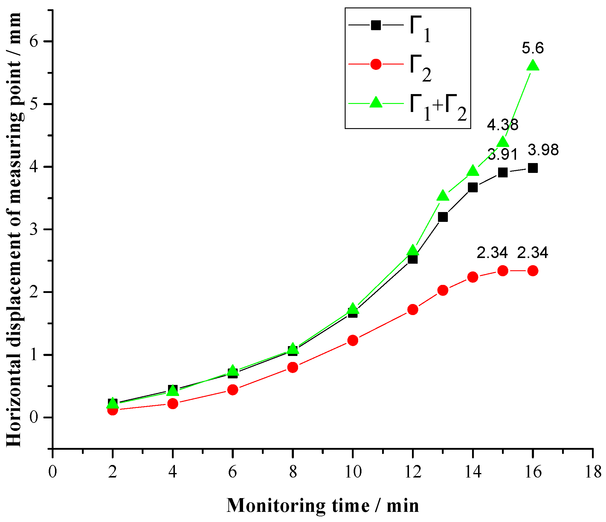
3.1. Basic Assumptions of Risk Factor Coupling Coefficient
The coupling effect of risk factors is studied by using conditional probability. Firstly, the coupling coefficient of risk factors is defined and meets some basic assumptions. The minimum causal unit is assumed, as shown in
Figure 1. Event C is the result, event Γ
1 (c) and Γ
2 (c) is the factor causing event C, abbreviated as Γ
1 and Γ
2.
Figure 1a shows the case with only one factor and
Figure 1b shows the case with two factors. It is assumed that the system in
Figure 1a is
and
Figure 1b is
. On this basis, the following assumptions are made, as shown in
Table 1.
Assumption 1. When the risk factors (Γ) do not exist, the system risk is 0.
During risk analysis, according to the amount of information available, an event
C may be in three states of “occurred”, “not occurred” and “uncertain”, which are respectively expressed as:
When discussing a set of
n events, there may be 3
n possible state combinations for the events in this set, which is called a “situation”. “No risk factors occur” refers to a situation in which all the causes obtained through causal analysis are in the state of non-occurrence. Which is expressed as:
All factor events in
Figure 1 Γ
i(
c) is the obvious cause of the result event
C, so when all factors do not occur, the occurrence probability of event C should be the basic probability
BPc0 determined by the hidden cause. However, under the condition of relatively complete causal analysis, the basic probability
BPc0 is generally small, and its impact on system risk is very limited. Therefore, for the sake of simplifying the model,
BPc0 = 0 can be assumed. Basic Assumption 1 can be expressed as:
Assumption 2. When a risk factor changes from non-occurrence to occurrence, the risk of the system will not be reduced.
The meaning of basic Assumption 2 is that risk factors are factors that have an adverse impact on system security, and the occurrence of a risk factor cannot make the system safer. In other words, comparing the risk of the system when the risk factor occurs with the risk when it does not occur, the former should be greater than the latter, or at least not less than the latter. Due to the relativity of risk factors, this nature should be established in all parts of the system. It can be inferred that when the risk factor occurs, the probability of all subsequent events is greater than when it does not occur. Under the condition of satisfying basic Assumption 1, basic Assumption 2 is naturally established in
and can be expressed as the following formula in
.
Assumption 3. Under the same objective situation, the risk of the system remains unchanged and has nothing to do with the result of causal analysis.
Basic Assumption 3 is closely related to the objective existence of risk factors. For the same result event
C, the causes of different causal analysis may be different, but these different analysis results objectively correspond to the same event. For example,
and
can be regarded as two different causal analyses of the same event, but both appear Γ
1 this factor. The following two situations exist in
and
respectively.
For any causal analysis example, the hidden cause is in an uncertain state. Due to factors Γ
2 is an explicit cause in
, but it exists as an implicit cause in
. Therefore, the second formula of Formula (5) corresponds to the same objective situation. Then, according to basic Assumption 3, the following formula holds:
Substitute Equation (4) into Equation (6) to obtain:
Assumption 4. When the state of all factors is unknown, the risk of a system will not be reduced after adding risk factors to the system without considering the coupling effect.
The causes of an event always exist objectively and are inexhaustible. The work of causal analysis is only to reveal and screen out the dominant factors in these causes. Then, adding risk factors to a system is essentially a further causal analysis. This behavior only reveals more information in the system without any interference with the system itself. Therefore, the system risk should remain unchanged in this case. The above expression can be expressed as:
where the angle mark “
Ω” represents that the system is in any condition. Substituting Equations (3) and (6) into Equation (9), we can get:
This result is undoubtedly unreasonable. Through the analysis, it can be found that the reason for this result is the simplification of the basic probability in basic Assumption 1, which is not in line with the objective situation. This term in Equation (10) is rounded off by basic Assumption 1 as part of the basic probability in
, but in
, this part of the probability is explicitly expressed because
changes from implicit cause to explicit cause, resulting in this unreasonable result. If the basic probability rounded off by basic Assumption 1 is expressed as
and
in
and
respectively, Equation (9) can be rewritten as:
From the relationship between the basic probability and the completeness of causal analysis, we can know that
≥
. At the same time, after substituting Equation (6) into (11) and eliminating the term, we can get:
This result is reasonable. If we want to solve the logical problem in Equation (10) under the condition that basic Assumption 1 is true, a feasible method is to make Equation (10) an inequality. That is:
In the above assumptions, except basic Assumption 1, other assumptions are based on the basic concept of causality and probability theory and are derived through logical derivation. Based on the above basic assumptions, the coupling coefficient can be defined.


