Abstract
Electroencephalography (EEG) has been widely used in the research of stress detection in recent years; yet, how to analyze an EEG is an important issue for upgrading the accuracy of stress detection. This study aims to collect the EEG of table tennis players by a stress test and analyze it with machine learning to identify the models with optimal accuracy. The research methods are collecting the EEG of table tennis players using the Stroop color and word test and mental arithmetic, extracting features by data preprocessing and then making comparisons using the algorithms of logistic regression, support vector machine, decision tree C4.5, classification and regression tree, random forest, and extreme gradient boosting (XGBoost). The research findings indicated that, in three-level stress classification, XGBoost had an 86.49% accuracy in the case of the generalized model. This study outperformed other studies by up to 11.27% in three-level classification. The conclusion of this study is that a stress detection model that was built with the data on the brain waves of table tennis players could distinguish high stress, medium stress, and low stress, as this study provided the best classifying results based on the past research in three-level stress classification with an EEG.
1. Introduction
The psychological quality of competition sports players is critical for them to achieve peak performance, but psychologically, they are liable to stress regardless of everyday stresses or the stresses of competition [1,2]. While appropriate levels of stress help men and women achieve optimal performance, improper stresses impair performances [3,4,5]. When a person is subject to external stimulation that threatens the balance within his/her body, an adaptation of physical and mental status emerges; in that sense, stresses are an adaptive reaction [6]. Despite different sources of stress, in order to maintain a physical–mental balance, certain similar physiological reactions occur in people due to stress: the secreted adrenaline increases, along with increased heartbeats, fast breathing, increased blood pressure, increased blood sugar content, and other changes [7]. Though stresses cannot be measured directly, individual physiological reactions and changes can be detected through physiological parameters such as electroencephalography (EEG), electrocardiography (ECG), and electromyography (EMG) to analyze the status of stresses to which the individuals are subject [8].
Stressors are the stimulative contexts that cause stress reactions and can be applied in stress detection. The Stroop color and word test (SCWT) was, at first, widely used in experiments of clinic research of neuropsychology and then discovered to induce an increase in adrenaline, heartbeats, respiratory rates, anxiety, etc., which are all that emerge as a result of stress reactions caused by stressors and, thus, can be effectively applied in stress detection [9,10,11]. In the Montreal imaging stress task (MIST), which originated from the Trier social stress test (TSST), difficulty in mental arithmetic (MA) and a time limit were used in the experiment groups, and it showed a significant increase in the level of cortisol in saliva compared with the control groups and the rest groups. Cortisol is also called a stress hormone, as cortisol begins to increase when stressors appear, with the effect of increasing the blood pressure and blood sugar. Hence, MIST can serve as a tool for stress detection to be used in research on the influences of social–psychological stresses [12].
EEGs reflect the psychological and physiological status of a person. EEG measurements work to detect the stress condition of a subject promptly, making an objective and quantifiable assessing tool [13]. However, the original signals of brain waves have a low signal-to-noise ratio (SNR), are not stable signals, and have high variations among individuals; thus, how to analyze the physiological signals from the brain is an important issue in increasing the accuracy of stress assessments [14]. According to the International Federation of Clinical Neurophysiology (IFCN), by the most common categories, the frequencies of brain waves, are divided, from low to high, into the Delta band (0.1–<4 Hz), the Theta band (4–<8 Hz), the Alpha band (8–13 Hz), the Beta band (>13–30 Hz), and the Gamma band (>30–80 Hz) [15]. Delta waves represent the sleeping status of a person; Theta waves a shallow sleeping status; Alpha waves a relaxed and calm status; and Beta waves the statuses of thinking, working, tension, anxiety, or stress.
Over recent years, EEG was widely used in research regarding stress detection. The authors of [16] used the exercises memory search, SCWT, and public speech as stressors, with sources of records, including a heart rate monitor (HRM), electrodermal activity (EDA), respiratory changes, and EEG. An independent component analysis (ICA) was used to eliminate artifacts from the EEG, a 4–400 Hz band pass filter to rule out undesired bands, and last, the framework of a convolutional neural network (CNN) in combination with long short-term memory (LSTM) to perform two-level classification with an accuracy at 90%. When using only EEG features, they achieved an 87.5% accuracy. In the research [17], a novel wearable device that is capable of measuring both the ECG and EEG was designed, and two stress sources, which were SCWT and MA, were used for recording the heart rate variability (HRV) and EEG. EEG signals were put to calculations with fast Fourier transform (FFT) into a power spectral density (PSD) to allow the extraction of features from the resultant PSDs of each band (Delta, Theta, Alpha, and Beta); the features selected by the analysis of variance (ANOVA) were classified by the support vector machine (SVM) with an accuracy at 77.9%. The authors of [18] employed MA tasks to cause a stress state, where ECG, breath signals, blood volume pulse (BVP), and EEG were extracted. From EEG, the physiological signals contained in brain waves of 14 channels on Delta, Theta, Alpha, and Beta bands were extracted. When using the random forest as the classifier on only the features provided by EEG data, the accuracy of distinguishing between resting and stressed states was 96.0%.
In research [19], computer-based MA was used to induce stresses, which, and control conditions too were divided into four levels of difficulty. The features extracted from EEG signals were absolute power, relative power, coherence, phase lag, and amplitude asymmetry. They began by standardization with a z score, then used receiver operating characteristic curve (ROC), t-test, and Bhattacharya distance for feature selection, and finally used logistic regression, SVM, and Naive Bayes to classify. Their findings suggested that a two-level stress classification achieved a 94.6% accuracy. The authors of [20] used MA, memory image, and public speech as the tests for stress-inducing tasks and resulted in ECG and EDA records. The results of the experiment indicated that the use of single-channel EEG features landed an optimal accuracy in classification between relaxed and high brain load states at 86.66%. The authors of [21] used EEG of 14 channels of brain waves on Alpha and Beta bands and combined with SCWT and MA. The brain waves collected by SCWT were those of a relatively low-stressed state, and those collected by MA were of a relatively high-stressed state. Last, SVM was employed to discern the indicators for brain waves stress levels. The accuracy for three-level stresses was 75%, and those for two-level stresses were 88% and 96% in the cases of SCWT and MA. The authors of [22] utilized SCWT as a stressor to induce four levels of stress and extracted combinations of features from EEG signals, including fractal dimensions and statistical features; the use of SVM as a classifier was able to identify two-level, three-level, and four-level stress classifications, where the accuracy for two-level stresses was 85.17%.
Past documents suggested that the measurements by different methods of mental stresses through EEG usually involved three stages, namely, data collection, data preprocessing, and classification [16,17,18,19,20,21,22]. (1) Data collection: in regard to short-term stresses, stressors are used to induce acute stresses, e.g., SCWT [16,17,21,22] and MA [17,18,19,20,21]. (2) Data preprocessing: intended to eliminate artifacts and noises and to extract useful features, where the methods available for eliminating artifacts and noises are the ICA and filters. (3) Classification: as classifiers, there is machine learning [17,18,19,20,21,22] and deep learning [16].
Machine learning is one of the core areas of artificial intelligence, which is the study of how to create algorithms that are capable of learning from experiences and improving their own ability, dissimilar to the algorithms that simply operate by given specific rules [23]. Machine learning is based on the study of statistical probabilities and computer science; employs algorithms such as logistic regression, SVM, decision tree, multilayer perceptron (MLP), and K-Nearest Neighbor (KNN); and has been applied in various fields, including physiological signals, medicine, industry, agriculture, and mail management [24,25].
Deep learning is a subfield of machine learning that uses deep neural networks as an architecture. CNN are currently the most widely used models in deep learning. In 1998, LeNet [26] laid the basic framework for CNN, which consists of convolutional layers, pooling layers, and fully connected layers. AlexNet [27] won the classification task in the 2012 ImageNet Large Scale Visual Recognition Competition (ILSVRC). Since then, deep learning has developed rapidly, including VGG [28], GoogLeNet [29], ResNet [30], InceptionResNetV2 [31], etc. In 2018, BERT (Bidirectional Encoder Representations from Transformers) achieved good results in NLP (Natural Language Processing) tasks [32]. The Transformer network structure is based on the attention mechanism. At present, the network structures mainly include MLP (multilayer perceptron), CNN, RNN (recurrent neural network), and Attention, which can be combined. Deep learning has been applied to the EEG for the mental workload, emotion recognition, motor imagery, event-related potential detection, etc. [33,34,35].
Taiwan’s table tennis is famous worldwide, and it is also one of the critical projects in developing sports in Taiwan. Studying table tennis players’ psychological stress can help manage stress and improve the sport performance. Compared with other sports, table tennis is a fast, precise, and open sport.
Since the original signals of brain waves have many noises and errors tend to arise during the process of signal extraction, how to extract and analyze EEG signals is an important issue for increasing the accuracy in stress assessment [14]. Therefore, this study uses different extraction methods and analysis methods to improve the accuracy of stress assessment. This study aims to collect EEG data of competition table tennis players by SCWT and MA and analyze brain waves by using machine learning and build models for stress classification, in which the stress classifying models include generalizing and personalizing ones to distinguish high, medium, and low stresses.
In this study, the EEG of table tennis players was collected by using SCWT and MA and analyzed by algorithms of machine learning; our experiment revealed XGBoost as the optimal model. The research findings indicated that, in three-level stress classification, XGBoost had an 86.49% accuracy in the case of the generalized model. This study outperformed other studies by up to 11.27% in three-level classification.
2. Materials and Methods
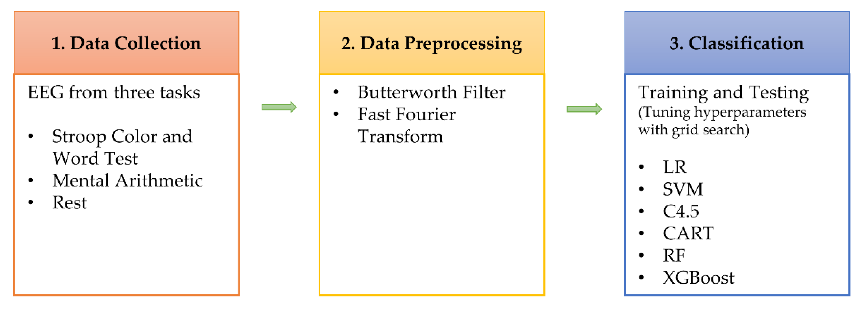
The experiment process of this study is as Figure 1 shows, comprising three stages: data collection, data preprocessing, and data analysis. In the data collection stage, EEG data at rest, SCWT, and MA were collected using an electroencephalograph. The data preprocess stage rules out undesired signals and transforms the data from the time domain into the frequency domain. The data classification stage performs feature analysis using machine learning and builds generalizing and personalizing stress models. The hyperparameters of the model are tuned using a grid search. A generalizing stress model is a stress detection model built by mixing the data of all persons, while a personalizing stress model is a stress detection model built based on personal data.
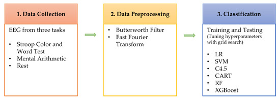
Figure 1.
Diagram for the research flow.
2.1. Data Collection
2.1.1. Participants
We recruited 26 Class A table tennis players (there are 12 male players) at the National Taiwan University of Sport as participants, and we considered only those without brain neural diseases. Their age was 20 ± 1.3 years. Before the research began, we outlined the experiment process to them, and they also signed the description and consent on human research form. This study was approved by the First Human Research Ethics Review Board affiliated with the College of Medicine, National Cheng Kung University (A-ER-108-041).
2.1.2. Stress Test
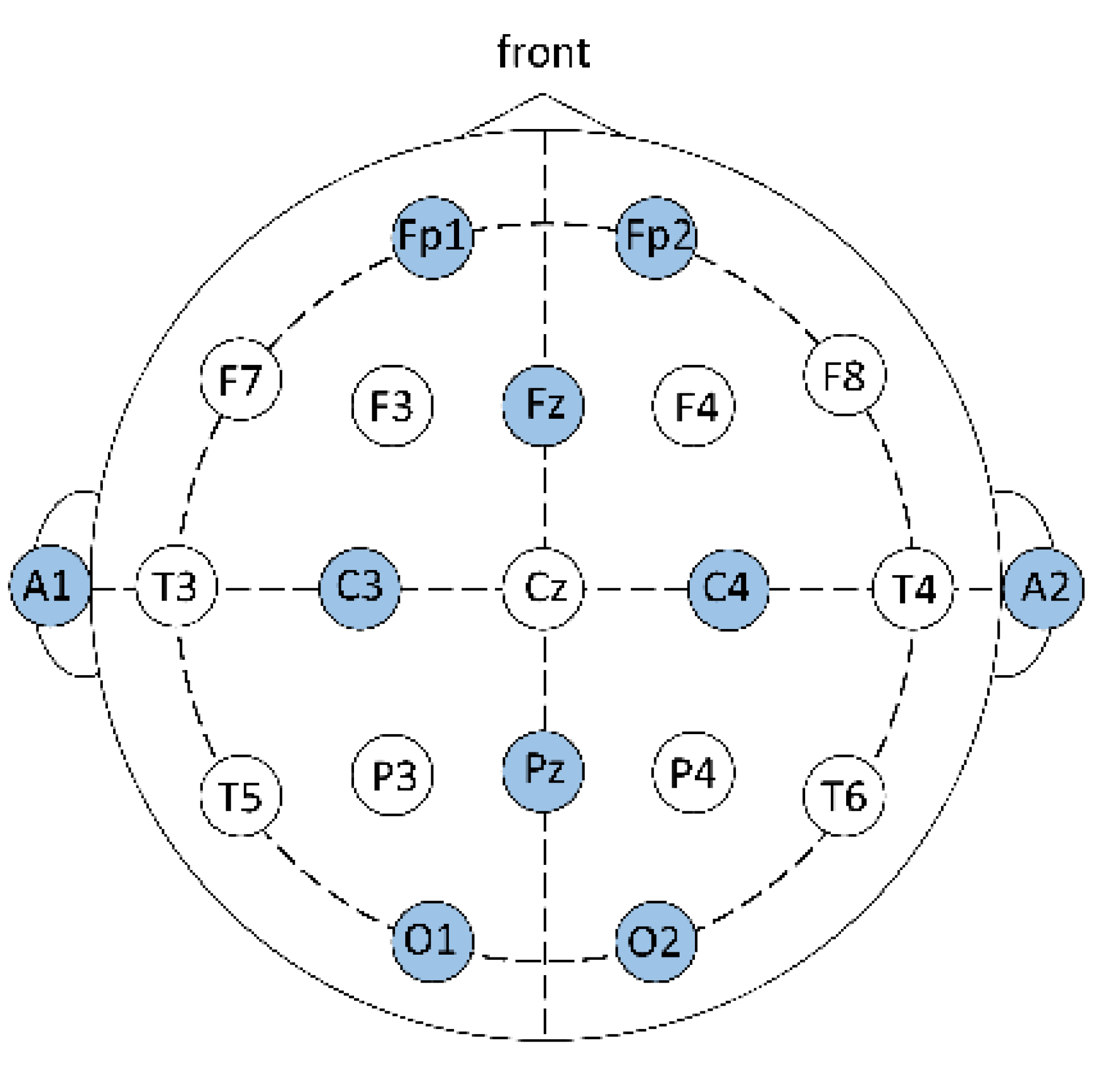
In the table tennis training hall, the participants wear an electroencephalograph, which is Portable 40—the lead system of recording neural image electric potential—with the leads, onto which conductive glue is applied, attached to the scalp. The resistance at every electrode position should be under 5 Ω, the sampling frequency is 1024 Hz, and the intensity of brain waves is μV signals. The stress test is conducted to gather changes in electric potential on the scalp. For the electrode positions, the international 10–20 system is used [36,37], as Figure 2 shows.

Figure 2.
International 10–20 system, with the designator Fp corresponding to the frontal polar area of the brain, F to the frontal area, C to the central area, P to the parietal area, O to the occipital, T to the temporal area, and A to the auricular area. In this study, a total of 10 electrode positions on the head are recorded; they are Fp1 (left frontal lobe electrode), Fp2 (right frontal lobe electrode), Fz (frontal midline), C3 (left central), C4 (right central), Pz (middle line of vertex), O1 (left occipital lobe), O2 (right occipital lobe), A1 (left auricular), and A2 (right auricular), of which A1 and A2 are the reference electrodes.
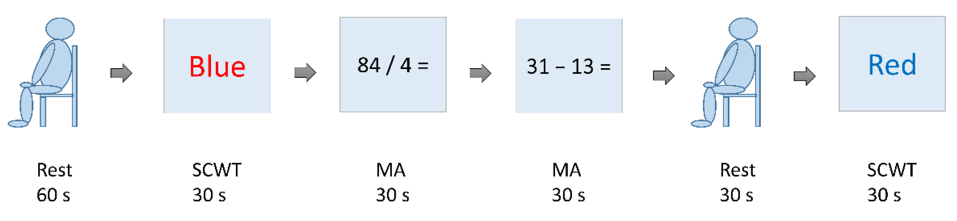
The stress test is a test designed with reference made to Reference [21] and includes the SCWT and MA. Prior to the formal test, we would collect the brain waves in a resting state for 60 s and allow the subjects to practice once on the SCWT and MA. The formal test includes the following sequence: SCWT, MA, MA, black screen (participant at relaxed rest), and SCWT, as Figure 3 shows. The participants would not be informed of the sequence. The time for each test is 30 s. The time between two tests is 20 s. In this study, the EEG data were collected during the formal testing of the SCWT and MA.
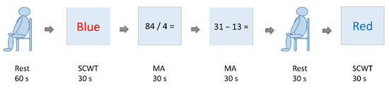
Figure 3.
Diagram for the stress test.
With the SCWT, new words appear on the screen at three-second intervals; these testing words come in random combinations of colors among red, blue, green, and yellow and a font type. The participants are required to choose correctly the color they see in the words on placards. The brain wave data collected at this test are of high stress compared with the rest state but are of a medium-stress state when compared with the brain waves of a low-stress state in the MA test.
With MA, questions of arithmetic (addition, subtraction, multiplication, and division) with numbers in the range of 1 to 1000 appear on the screen at five-second intervals, where the participants should complete responses by MA. The brain waves collected at this test are those of a high-stress state if compared with the SCWT.
2.2. Data Preprocessing
2.2.1. Filter
The Butterworth filter is used to extract the signals of a certain range of frequencies. As brain wave signals are weak and susceptible to interference when being gathered, a filter is needed to screen out unwanted frequency bands. To remove lower bands, a low-pass filter can be used to block the frequencies in certain bands; to remove higher bands, do otherwise. In this study, the Butterworth filter (BF) is used to remove the bands above 70 Hz to capture the 0–70 Hz band, as well as to eliminate a certain baseline shift due to external factors. The amplitude and frequency relationship of the Butterworth low-pass filter is defined in Formula (1):
where is the transfer function, is the order of the filter, is the Imaginary unit, is the angular frequency, and is the cutoff frequency.
2.2.2. Feature Extraction
Signal processing and analysis methods are divided into two types: time domain and frequency domain. The time domain analysis is time-based and observes signal variations on the time axis. In this study, the time domain signals are converted by FFT into amplitudes of multiple bands to form PSD in order to capture the PSDs of different brain wave bands. FFT is a fast algorithm for discrete Fourier transform (DFT). The calculation of DFT is defined as Formula (2):
where is the discrete frequency signal, is the discrete time signal, and is the number of samples.
During the stress test, the time domain signal is 30 s for each test or 60 s of rest before the test is obtained. The conversion of the time domain signals by FFT organizes and obtains 8 bands per second, namely, Delta (0–<4 Hz), Theta (4–<8 Hz), Low Alpha (8–<10 Hz), High Alpha (10–<13 Hz), Low Beta (13–<20 Hz), High Beta (20–<30 Hz), Low Gamma (30–<46 Hz), and High Gamma (46–70 Hz). Every one of the 8 electrode positions corresponds to these 8 bands (such as Fp1_HighAlpha, Fp1_LowAlpha, etc.), resulting in a total of 64 features, and the unit is µV/√Hz.
2.3. Classification
Data classification utilizes the algorithms of logistic regression, SVM, decision tree C4.5, classification and regression tree, random forest, and extreme gradient boosting (XGBoost) in machine learning and builds stress detection models.
2.3.1. Logistic Regression (LR)
LR takes logarithms of the odds ratio, which further undergo transformation with the Sigmoid function, to create regression equations on the assumption that the conditional probability distributions of the dependent variables subject to independent variables are a Bernoulli distribution instead of non-normal distribution [38]. This is a model capable of leading to dichotomous results to determine the “probability of a certain sample belonging to a certain category” as the basis for classification. The LR model is Formula (3):
where is the conditional probability, is the output, is the input feature vector, is the weight vector, and is the bias.
2.3.2. Support Vector Machine (SVM)
SVM is a supervised learning method. Support vectors serve to identify an optimal hyperplane for classification, such that the margins between two categories are maximized to be able to separate them by maximal intervals, also allowing calculations using kernel functions at low dimensions before displaying classification results at higher dimensions to deal with nonlinear problems [39]. The advantages of SVM are higher abilities specific for small samples, nonlinearity, and high dimensions. Its drawbacks are the difficulty of choosing kernel functions and sensitivity to deficiencies. Given the difficulty of choosing kernel functions, it is possible to attempt different kernel functions in order to find the appropriate kernel functions. The SVM model is Formula (4):
where is the Lagrange multiplier of the th training sample, is the output of the th training sample, is the th training sample, is the novel sample, is the bias, and is the number of training samples.
The model of the SVM using the kernel function is shown in Formula (5):
where is the Lagrange multiplier of the th training sample, is the output of the th training sample, is the th training sample, is the novel sample, is the bias, is the number of training samples, and represents the kernel function. The kernel functions include a linear, polynomial, radial basis and so on.
2.3.3. Decision Tree C4.5 (C4.5)
C4.5 was improved based on the ID3 algorithm [40]. C4.5 uses a gain ratio as the branching criteria, where branch attributes are chosen by means of the randomness difference between parent nodes and child nodes and the amount of split information. As the gain ratio is the ratio of information acquired to the split information, we will first describe the information gain and split information. means that attribute will profit from the information divided by dataset , as shown in Formula (6):
where represents the information entropy of dataset , represents the th value of different values of attribute , represents how many different values there are, represents the number of subsets contained in the th value, represents the number of datasets , and represents the information entropy of dataset .
represents the split information of attribute for the dataset split, as shown in Formula (7):
where represents the th value of attribute , represents how many different values there are, represents the number of subsets contained in the jth value, and number of datasets .
represents the gain ratio of attribute to the division of dataset , as shown in Formula (8):
where is the information gain of attribute splitting dataset , and is the split information of attribute splitting dataset .
2.3.4. Classification and Regression Tree (CART)
CART is a binary tree classification algorithm; it uses the Gini coefficient as the branching criteria, where the features most suitable for branching are identified by comparing impurities of the features [41]. A feature whose impurity decreased by the most significant difference is the branching feature of the decision tree. The algorithm comprises four steps as follows:
- Determine the Gini coefficient for all the feature values of all the features in the dataset and select the optimal feature and splitting point with the smallest Gini coefficient;
- Generate two branches on both sides based on the optimal feature and the optimal splitting point to divide the dataset into two branch datasets side by side;
- Calculate the two branch datasets, where, if the Gini coefficient is smaller than the threshold or the number of samples is smaller than the threshold or there are no features, the node ceases to recur;
- Repeat Steps 1–3 on the modes of the two branches to generate a CART decision tree.
The Gini coefficient means impurity, whereas a smaller Gini coefficient means a higher purity, implying a better effect of the classification.
represents the Gini coefficient of the dataset , such as Formula (9):
where represents the th category, represents the total number of categories, and represents the probability that the th category appears in the dataset .
represents the Gini coefficient of attribute A partitioning dataset D, such as Formula (10):
where j represents the jth value of attribute , represents how many different values there are, represents the number of subsets contained in the th value, is the number of datasets , and represents the Gini coefficient of dataset .
2.3.5. Random Forest (RF)
RF is an algorithm consisting of multiple classifiers of a decision tree (usually using CART), and its output categories are according to a majority vote of those of individual output categories [42]. Compared with conventional decision trees, RF has many advantages, e.g., creating high-accuracy classifiers for many types of data, handling massive input variables, and the importance of assessing the variables in deciding types.
2.3.6. Extreme Gradient Boosting (XGBoost)
XGBoost was developed from a gradient boosting decision tree (GBDT) [43]. GBDT is an addition model (serial integration) comprising multiple CART trees, each of which leans on the residuals from the sum of the conclusions of all previous trees, as in Formulas (11) and (12). The step includes multiple iterations, each creating a decision tree in order to continually decrease residuals to increase the precision. XGBoost exercises 2-order Taylor expansion on loss functions to increase the precision, where regular items are incorporated in objective functions to decrease the variance of the model, and uses feature sampling to prevent overfitting. Its advantages are a higher precision and prevention from overfitting; and its drawback is depleting computing resources by the presorting process.
where is the currently fitted tree, is the best output value of the fitted leaf node, is the loss function, is the number of samples, and is the actual value of the th sample.
where is the current ensemble of all trees, is the input sample, is the ensemble of all trees so far, and is the currently fitted tree.
3. Results and Discussion
3.1. Brain Wave Dataset
In this study, brain wave data of 25 regularly trained players were collected. Since one person’s information was incomplete, it was removed, resulting in a total of 4433 records of data from all the subjects. Additionally, other attributes of stress were incorporated based on the stress classification in our experiment as indicators of high, medium (mid), and low stresses. In the end, each record of data included eight electrode positions (Fp1, Fp2, Fz, C3, C4, Pz, O1, and O2), each of which had the electrode data on eight frequency bands (Delta, Theta, Low Alpha, High Alpha, Low Beta, High Beta, Low Gamma, and High Gamma) (in µV/√Hz); that was 64 attributes. An additional stress indicator made a total of 65 attributes. Of all the attributes, the brain wave data of the frequency bands were continuous data, while the stress levels and player groups were discrete data.
The brain waves at a resting state prior to the test served as the data for low stress (1476 records), the SCWT as mid-stress data (1469 records), and MA as high-stress data (1488 records). The labeling method, when classifying rest, SCWT, and MA, was set to 0, 1, and 2, respectively; when classifying rest and SCWT, the label was set to 0 and 1, respectively; and when classifying rest and MA, the label was set, respectively, to 0 and 1.
3.2. Evaluation Metrics
A Confusion matrix is a matrix for statistical work on the correctness or incorrectness of classification. In the case of two-level classification, there are four types of results, namely, True Positive (TP): correctly predicting a positive sample as positive, True Negative (TN): correctly predicting a negative sample as negative, False Positive (FP): incorrectly predicting a negative sample as positive, and False Negative (FN): incorrectly predicting a positive sample as negative.
The commonly used assessing indicators are described next. Accuracy (Acc), which is the proportion of correctly predicted samples to the total predicted samples, as Formula (13) shows. Precision (Pre), which is the proportion of correctly predicted positive samples to the total samples predicted as positive, as Formula (14) shows. Recall (Rec), which is the proportion of correctly predicted positive samples to the total actual positive samples, also called the true positive rate (TPR), as Formula (15) shows. The F1-score (F1), which is the harmonized means of precision and recall, as Formula (16) shows. The Matthews correlation coefficient (MCC), which consists of all four types of the Confusion matrix (TP, TN, FP, and FN) and, thus, is a more balanced indicator for all types, as Formula (17) shows. In multi-level classifications, only the indicators of two-level classification that can be used would differ according to the way of the calculations; the method of this study is to determine, straightforwardly, the means of assessing indicators of different types added together.
The 10-fold cross-validation is a sampling of many times technique capable of minimizing the bias and variance of datasets and avoiding the overfitting problem. In 10-fold cross-validation, a dataset is randomly divided into ten subsets, of which one is used as a test set and the rest as a training set; when all subsets have been run once, their evaluation indicators are determined by a predicted value and real value. The mean measures are determined to obtain the final validation of the models [44].
In order to assess the results of the performance validation of the models, the 10-fold cross-validation was used in this study, along with a variety of model assessing indicators, which were five in the two-level classification, including accuracy, precision, recall, F1, and MCC, or four in the three-level classification, including accuracy, precision, recall, and F1.
3.3. Performance Evaluation of Classification Models
In this study, the algorithms of LR, SVM, C4.5, CART, RF, and GXBoost were used for comparison (see Table 1 for the parameters for the model), and a generalizing and a personalizing stress model were built. The generalizing stress model is a stress detection model built by mixing the data of all persons, whereas the personalizing stress model is one built based on their individual data. For the analytic results of stress classification, see Table 2, Table 3, Table 4, Table 5, Table 6 and Table 7 and Figure 4, Figure 5, Figure 6 and Figure 7.

Table 1.
Table of the model parameters.
Table 2.
Generalizing model for the three-level stress classification.
Table 3.
Generalizing model for the two-level stress classification (high and low stresses).
Table 4.
Generalizing model for the two-level stress classification (mid and low stresses).
Table 5.
Personalizing model for the three-level stress classification (mean of all).
Table 6.
Personalizing model—GXBoost three-level stress classification (top five individuals).
Table 7.
A comparison of this study and past studies.

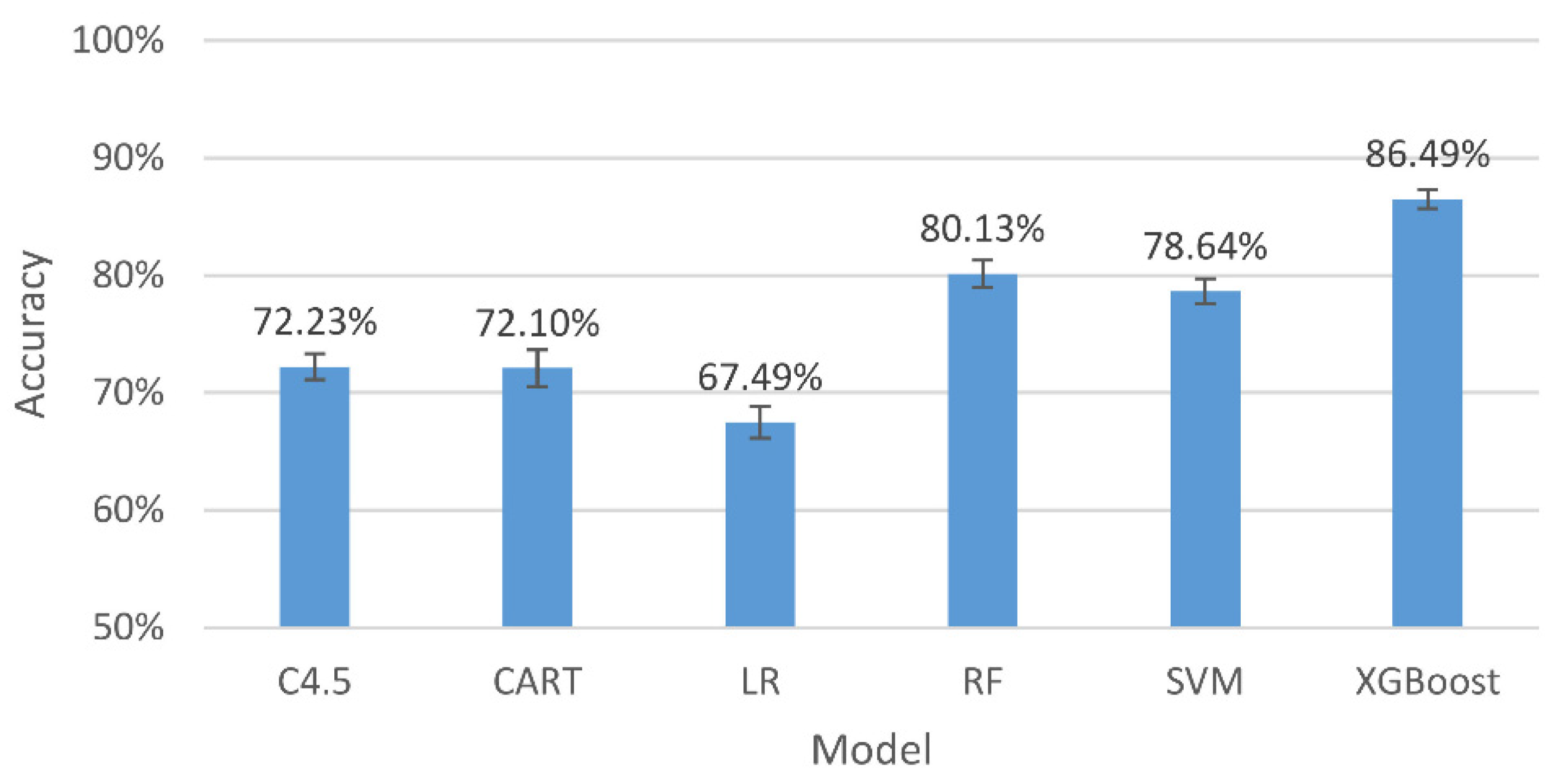
Figure 4.
The accuracy and 95% confidence intervals of the generalizing models for the three-level classification.

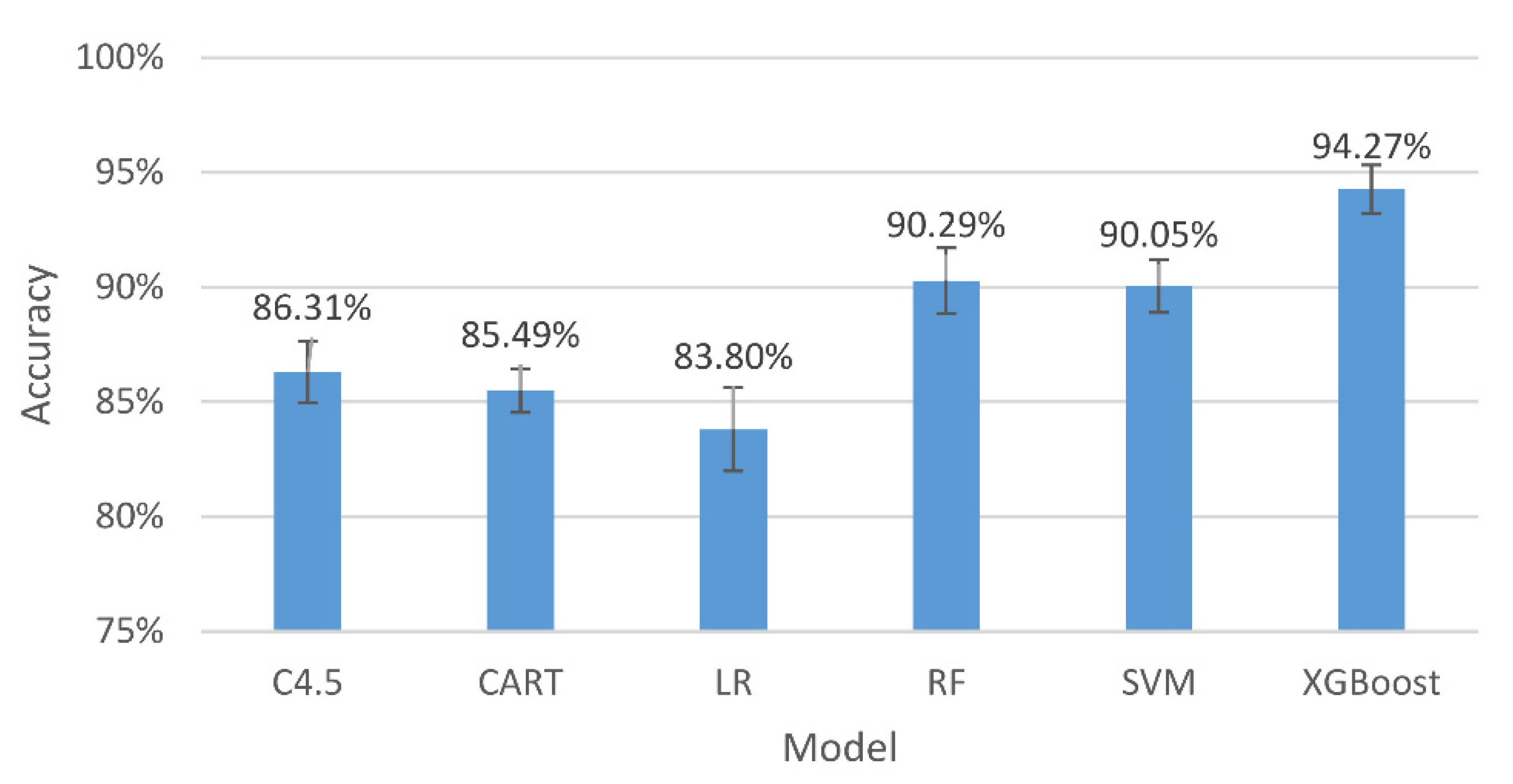
Figure 5.
The accuracy and 95% confidence intervals of the generalizing models for the two-level classification (high and low stresses).

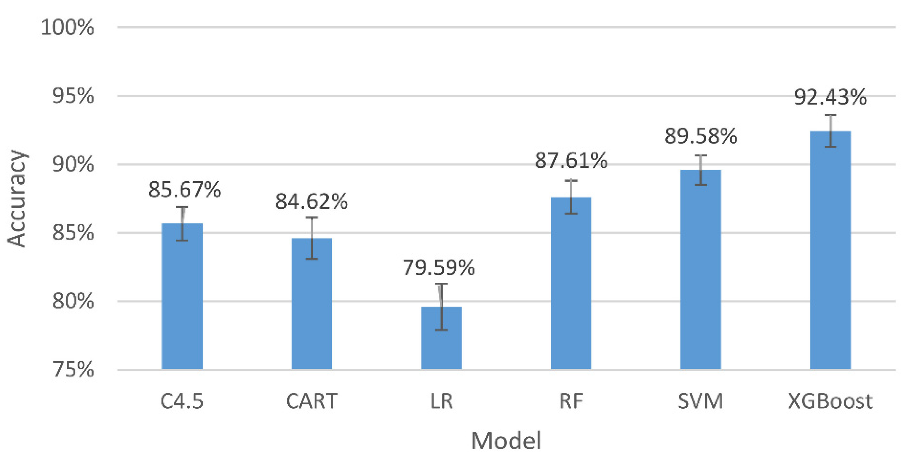
Figure 6.
The accuracy and 95% confidence intervals of the generalizing models for the two-level classification (mid and low stresses).

Figure 7.
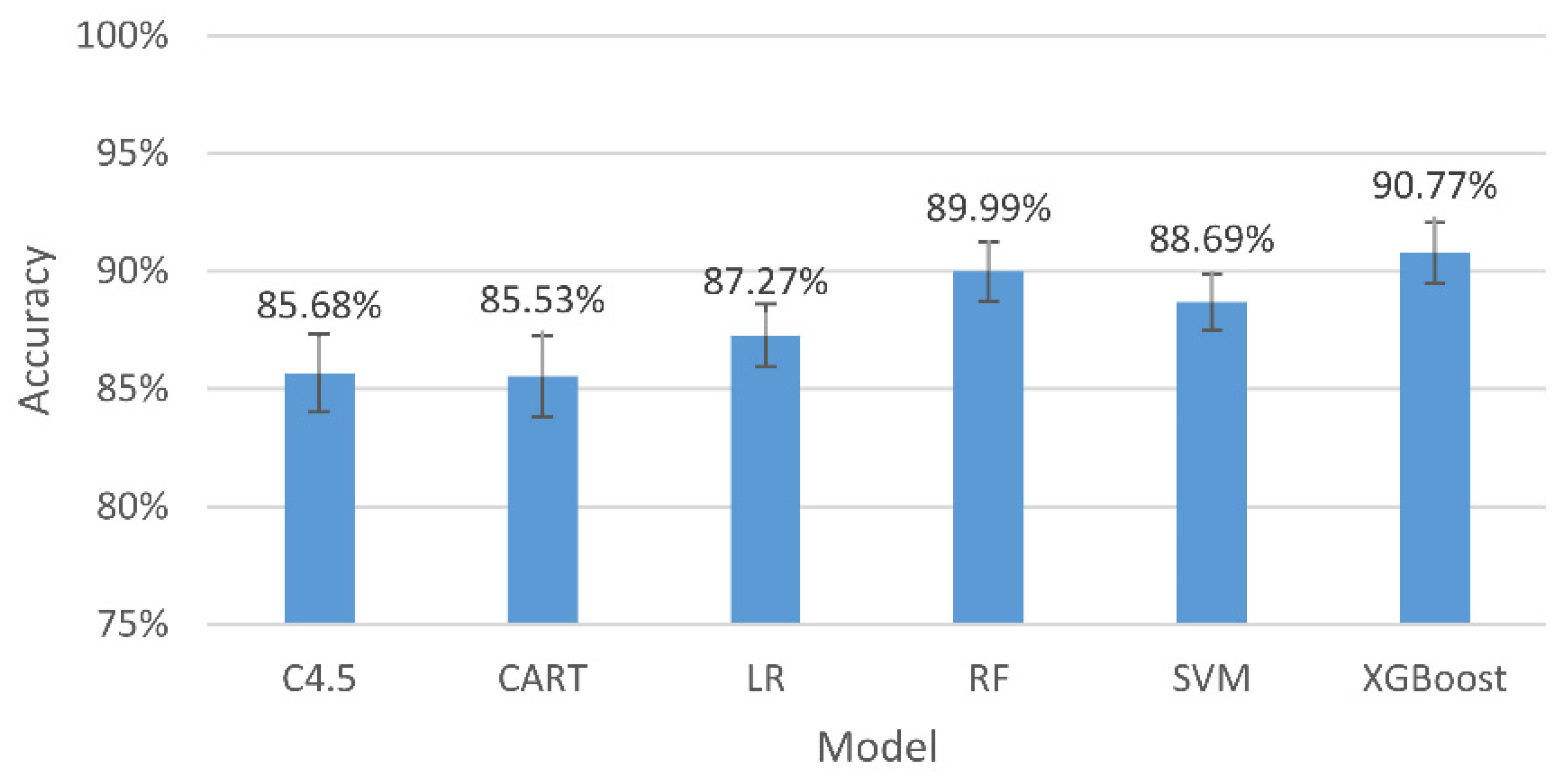
The accuracy and 95% confidence intervals of the personalizing models for the three-level classification (mean of all).
The results in Figure 4 indicate that, among all the assessing indicators, GXBoost is always the highest, with an accuracy of 86.49%.
The results in Figure 5 indicate that, among all the assessing indicators, GXBoost is always the highest, with an accuracy of 94.27%.
The results in Figure 6 indicate that, among all the assessing indicators, GXBoost is always the highest, with an accuracy of 92.43%.
The results in Figure 7 indicate that, among all the assessing indicators, GXBoost is always the highest, with an accuracy of 90.77%.
The results in Table 6 indicate that, among the 25 players, the one with the best accuracy was as high as 99.44%.
In this study, whether with the generalizing model or with the personalizing model, the best algorithm was always XGBoost. The three-level stress classification of the generalizing model had an accuracy of 86.49%. With the same model, the two-level stress classification between high and low stresses had an accuracy of 94.27% or an accuracy of 92.43% for the mid and low stresses. The three-level stress classification of the personalizing model had an average accuracy of 90.77%, with a top individual player hitting 99.44%. The personalizing model had higher accuracies than the generalizing model, because the instability of an individual’s brain waves, in addition to differences between the individuals, leads to lower accuracies in the classification with the generalizing model. Given that brain waves vary in individuals, if we could employ algorithms to identify the causes of those variances and eliminate them, we would be able to improve the accuracy of the classification with the generalizing model.
We compared the schemes proposed by past studies and the present one based on the number of subjects, channels, bands, features, stressors, classifier, and accuracy, as Table 7 shows.
We had the most subjects; yet, there were still under 30; it will be an option in the future to increase the number of subjects to make samples more representative and more powerful as evidence. For the classifier in this study, we adopted a relatively new algorithm of machine learning, XGBoost, whilst, in most of the other studies, the SVM classifier was used in the assessment. In this study, XGBoost always outperformed the SVM, whether with the generalizing model or with the personalizing model. Last, the three-level classification of this study had an accuracy of 86.49%, which excelled compared to other studies by as far as 11.27% in the three-level classification.
3.4. Key Feature of Stress Classification
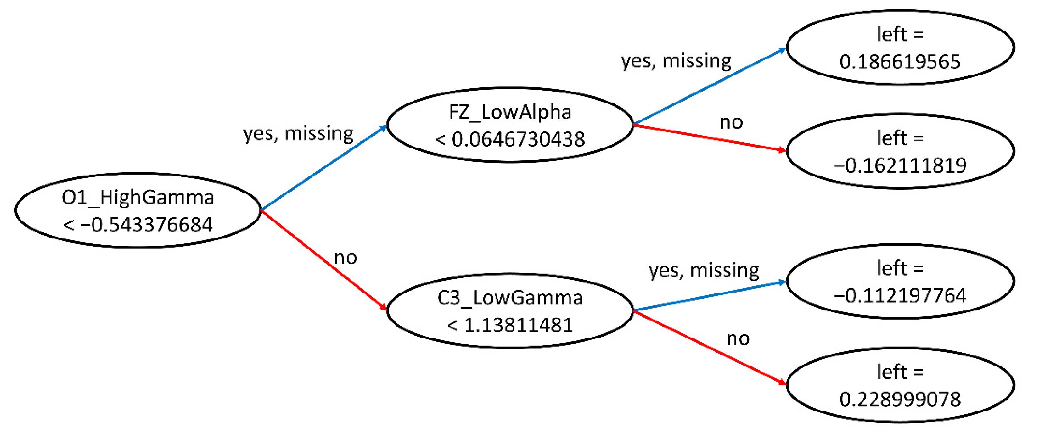
From the first CART decision tree for classifying stresses with the GXBoost algorithm in the generalizing model, we learned that the most important root node was O1_HighGamma (as Figure 8); therefore, we examined the box plot for O1_HighGamma during the exploratory data analysis, as shown in Figure 9.

Figure 8.
CART visualization.

Figure 9.
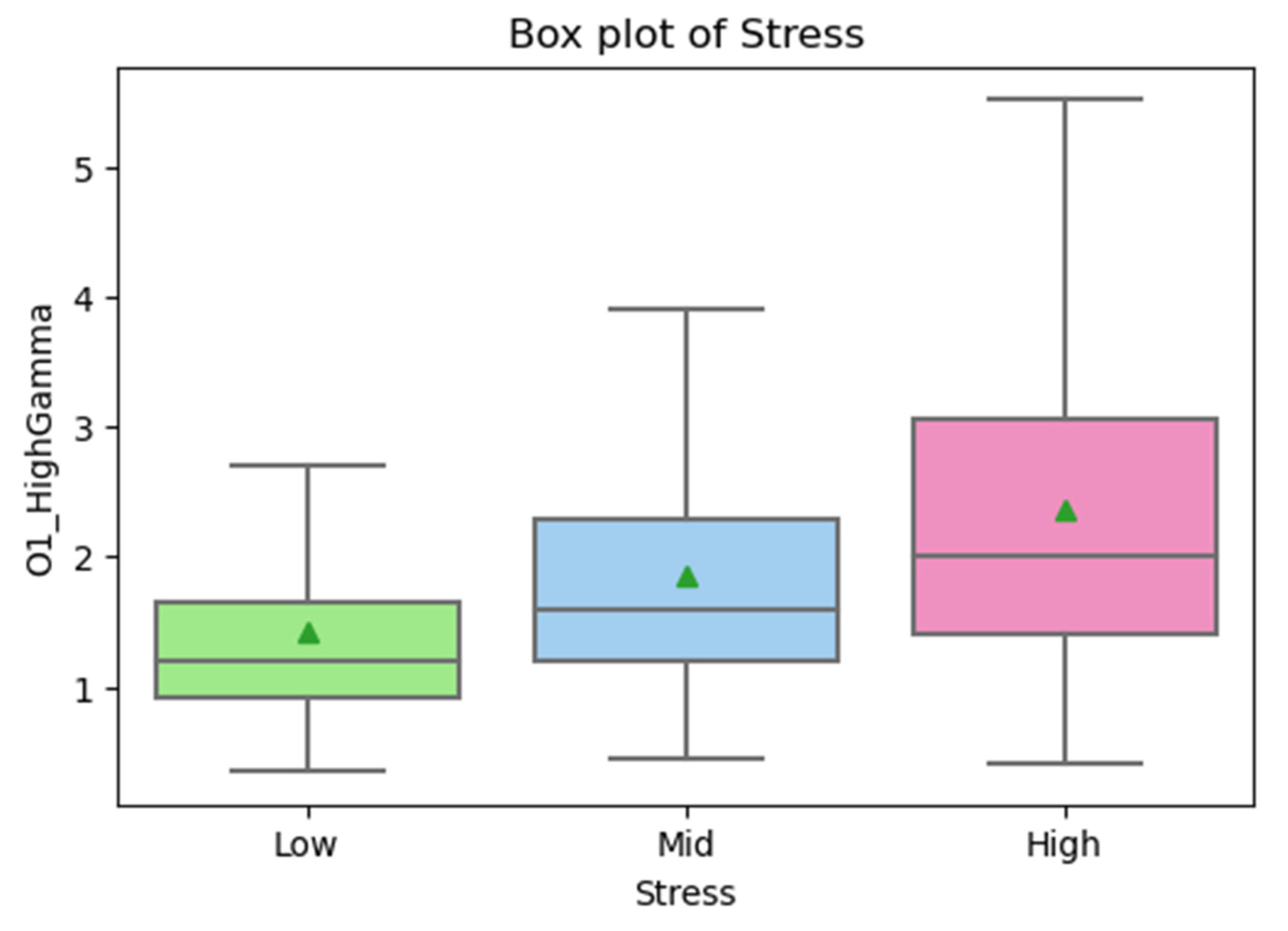
Box plot of O1_HighGamma.
The results in Figure 9 suggest that the X-axis is the stress levels, namely, high, mid, and low, and the Y-axis is the density of the power frequency spectrum in µV/√Hz, where the middle lines in the box are the medians, and the little triangles are the positions of the means. It is clear that the ranking of the means is high stress > mid stress > low stress. The means of the two types of O1_HighGamma attributes were compared using the independent sample t-test [45], and the results of the statistical analysis were as shown in Table 8.
Table 8.
Independent sample t-test on the O1_HighGamma features.
The results in Table 8 suggest that, in the data, the means of the high, mid, and low stresses had significant differences between one another. That verifies the possibility of causing different stress states by conducting the SCWT and MA.
Past studies suggested that Gamma waves are mainly associated with the extent to which minds are concentrated and lead to anxiety and stress [46]. Emotions are connected to Gamma waves [47,48,49], where the Gamma waves of negative emotions, in particular, are stronger than those of positive emotions [50]. Reference [51] stated that prefrontal lobe-corresponded Gamma power can serve as a biomarker for identifying stresses. The findings hereof indicated that a higher value of High Gamma at the O1 electrode position means higher stress, which is consistent with the literature and can serve as an important key feature for stress classification.
4. Conclusions
In this study, the EEG of table tennis players was collected by using the SCWT and MA and analyzed by algorithms of machine learning, namely, LR, SVM, C4.5, CART, RF, and XGBoost; our experiment revealed XGBoost as the optimal model. The stress models included the generalizing model and personalizing model, both providing the analytic results of stresses on players. This study outperformed other studies by up to 11.27% in the three-level classification. This study provided optimal classification results, which makes it different from other studies.
The number of players in this study was limited, and it is hoped to expand the samples of data in the future to at least 30 so that the samples will be more representative and more powerful as evidence, while the stress models will be generalizing in a better way. As brain waves vary from individual to individual, if we could utilize algorithms to identify the causes of such variations, we will improve the accuracies of classification with generalizing models. XGBoost has a good accuracy for low-dimensional feature data, but it is not suitable for processing high-dimensional feature data. In the future, it can be combined with deep learning, using deep learning to extract features and then using XGBoost for classification as the two are combined into a new model. The chief key feature of stress classification is High Gamma at the O1 electrode position, and this feature can serve as an important key feature in future research on psychological stresses. Last, this study employed the two different stressors of the SCWT and MA in the experiment, whereas the data from the lab context were limited and differed from those of the competition context that table tennis players face. It is possible in the future to collect data on brain waves during training or games to build stress models in competition contexts and to compare the differences thereof.
Author Contributions
Conceptualization, Y.-H.T., S.-S.Y. and M.-H.T.; Data curation, Y.-H.T.; Formal analysis, Y.-H.T. and S.-S.Y.; Funding acquisition, S.-K.W.; Investigation, Y.-H.T.; Methodology, S.-S.Y. and M.-H.T.; Project administration, Y.-H.T. and M.-H.T.; Resources, S.-K.W. and M.-H.T.; Software, Y.-H.T.; Supervision, S.-S.Y. and M.-H.T.; Validation, Y.-H.T. and M.-H.T.; Visualization, Y.-H.T.; Writing—original draft, Y.-H.T.; and Writing—review and editing, Y.-H.T., S.-K.W. and M.-H.T. All authors have read and agreed to the published version of the manuscript.
Funding
This research was funded by the Ministry of Science & Technology, R.O.C., grant number MOST109-2627-H-028-003.
Institutional Review Board Statement
The study was conducted in accordance with the Declaration of Helsinki and approved by the Institutional Review Board (or Ethics Committee) of the First Human Research Ethics Review Board affiliated with the College of Medicine, National Cheng Kung University (A-ER-108-041, 22 March 2019) for studies involving humans.
Informed Consent Statement
Informed consent was obtained from all subjects involved in the study. Written informed consent was obtained from the patient(s) to publish this paper.
Data Availability Statement
The labeled datasets used to support the findings of this study are available from the corresponding author upon request.
Acknowledgments
We are grateful to the National Taiwan University of Sport for providing us with the recruitment of the participants.
Conflicts of Interest
The authors declare no conflict of interest.
References
- Méndez-Alonso, D.; Prieto-Saborit, J.; Bahamonde, J.; Jiménez-Arberás, E. Influence of psychological factors on the success of the ultra-trail runner. Int. J. Environ. Res. Public Health 2021, 18, 2704. [Google Scholar] [CrossRef] [PubMed]
- Kim, E.J.; Kang, H.W.; Park, S.M. The effects of psychological skills training for archery players in Korea: Research synthesis using meta-analysis. Int. J. Environ. Res. Public Health 2021, 18, 2272. [Google Scholar] [CrossRef] [PubMed]
- Auer, S.; Kubowitsch, S.; Süß, F.; Renkawitz, T.; Krutsch, W.; Dendorfer, S. Mental stress reduces performance and changes musculoskeletal loading in football-related movements. Sci. Med. Footb. 2021, 5, 323–329. [Google Scholar] [CrossRef] [PubMed]
- Yadolahzadeh, A. The role of mental imagery and stress management training in the performance of female swimmers. Atena J. Sports Sci. 2021, 3, 1. [Google Scholar]
- Fradejas, E.; Espada-Mateos, M. How do psychological characteristics influence the sports performance of men and women? A study in school sports. J. Hum. Sport Exerc. 2018, 13, 858–872. [Google Scholar] [CrossRef]
- Selye, H. The Stress of Life; Mc Gran-Hill Book Company Inc.: New York, NY, USA, 1956. [Google Scholar]
- Selye, H. Stress and the general adaptation syndrome. Br. Med. J. 1950, 1, 1383–1392. [Google Scholar] [CrossRef]
- Li, Y.; Li, X.; Ratcliffe, M.; Liu, L.; Qi, Y.; Liu, Q. A real-time EEG-based BCI system for attention recognition in ubiquitous environment. In Proceedings of the 2011 International Workshop on Ubiquitous Affective Awareness and Intelligent Interaction, Beijing, China, 17–21 September 2011; pp. 33–40. [Google Scholar]
- Tulen, J.H.M.; Moleman, P.; Van Steenis, H.G.; Boomsma, F. Characterization of stress reactions to the Stroop Color Word Test. Pharmacol. Biochem. Behav. 1989, 32, 9–15. [Google Scholar] [CrossRef]
- Šiška, E. The stroop colour-word test in psychology and biomedicine. Acta Univ. Palacki. Olomuc. Gymn. 2002, 32, 45–52. [Google Scholar]
- Karthikeyan, P.; Murugappan, M.; Yaacob, S. Analysis of Stroop color word test-based human stress detection using electrocardiography and heart rate variability signals. Arab. J. Sci. Eng. 2014, 39, 1835–1847. [Google Scholar] [CrossRef]
- Dedovic, K.; Renwick, R.; Mahani, N.K.; Engert, V.; Lupien, S.J.; Pruessner, J.C. The Montreal Imaging Stress Task: Using functional imaging to investigate the effects of perceiving and processing psychosocial stress in the human brain. J. Psychiatry Neurosci. 2005, 30, 319–325. [Google Scholar]
- Giannakakis, G.; Grigoriadis, D.; Giannakaki, K.; Simantiraki, O.; Roniotis, A.; Tsiknakis, M. Review on psychological stress detection using biosignals. IEEE Trans. Affect. Comput. 2019, 3, 440–460. [Google Scholar] [CrossRef]
- Roy, Y.; Banville, H.; Albuquerque, I.; Gramfort, A.; Falk, T.H.; Faubert, J. Deep learning-based electroencephalography analysis: A systematic review. J. Neural Eng. 2019, 16, 051001. [Google Scholar] [CrossRef] [PubMed]
- Kane, N.; Acharya, J.; Benickzy, S.; Caboclo, L.; Finnigan, S.; Kaplan, P.W.; Shibasaki, H.; Pressler, R.; van Putten, M.J. A revised glossary of terms most commonly used by clinical electroencephalographers and updated proposal for the report format of the EEG findings. Revision 2017. Clin. Neurophys. Pract. 2017, 2, 170–185. [Google Scholar] [CrossRef] [PubMed]
- Masood, K.; Alghamdi, M.A. Modeling mental stress using a deep learning framework. IEEE Access 2019, 7, 68446–68454. [Google Scholar] [CrossRef]
- Ahn, J.W.; Ku, Y.; Kim, H.C. A Novel Wearable EEG and ECG recording system for stress assessment. Sensors 2019, 19, 1991. [Google Scholar] [CrossRef]
- Zanetti, M.; Faes, L.; De Cecco, M.; Fornaser, A.; Valente, M.; Guandalini, G.; Nollo, G. Assessment of mental stress through the analysis of physiological signals acquired from wearable devices. In Italian Forum of Ambient Assisted Living; Springer: Cham, Switzerland, 2018; pp. 243–256. [Google Scholar]
- Subhani, A.R.; Mumtaz, W.; Saad, M.N.B.M.; Kamel, N.; Malik, A.S. Machine learning framework for the detection of mental stress at multiple levels. IEEE Access 2017, 5, 13545–13556. [Google Scholar] [CrossRef]
- Secerbegovic, A.; Ibric, S.; Nisic, J.; Suljanovic, N.; Mujcic, A. Mental workload vs. stress differentiation using single-channel EEG. In CMBEBIH 2017; Springer: Berlin/Heidelberg, Germany, 2017; pp. 511–515. [Google Scholar]
- Jun, G.; Smitha, K.G. EEG based stress level identification. In Proceedings of the 2016 IEEE International Conference on Systems, Man, and Cybernetics (SMC), Budapest, Hungary, 9–12 October 2016; pp. 3270–3274. [Google Scholar]
- Hou, X.; Liu, Y.; Sourina, O.; Tan, Y.R.E.; Wang, L.; Mueller-Wittig, W. EEG based stress monitoring. In Proceedings of the 2015 IEEE International Conference on Systems, Man, and Cybernetics, Kowloon, China, 9–12 October 2015; pp. 3110–3115. [Google Scholar]
- Mitchell, T.M. Machine Learning; Mc Gran-Hill Book Company Inc.: New York, NY, USA, 1997. [Google Scholar]
- Panicker, S.S.; Gayathri, P. A survey of machine learning techniques in physiology based mental stress detection systems. Biocybern. Biomed. Eng. 2019, 39, 444–469. [Google Scholar] [CrossRef]
- Angra, S.; Ahuja, S. Machine learning and its applications: A review. In Proceedings of the 2017 International Conference on Big Data Analytics and Computational Intelligence (ICBDAC), Chirala, India, 23–25 March 2017; pp. 57–60. [Google Scholar]
- LeCun, Y.; Bottou, L.; Bengio, Y.; Haffner, P. Gradient-based learning applied to document recognition. Proc. IEEE 1998, 86, 2278–2324. [Google Scholar] [CrossRef]
- Krizhevsky, A.; Sutskever, I.; Hinton, G.E. ImageNet Classification with Deep Convolutional Neural Networks. In Proceedings of the 25th International Conference on Neural Information Processing Systems, Lake Tahoe, NV, USA, 3–6 December 2012. [Google Scholar]
- Simonyan, K.; Zisserman, A. Very Deep Convolutional Networks for Large-Scale Image Recognition. arXiv 2014, arXiv:1409.1556. [Google Scholar]
- Szegedy, C.; Liu, W.; Jia, Y.; Sermanet, P.; Reed, S.; Anguelov, D.; Erhan, D.; Vanhoucke, V.; Rabinovich, A. Going deeper with convolutions. In Proceedings of the IEEE Conference on Computer Vision and Pattern Recognition, Boston, MA, USA, 7–12 June 2015; pp. 1–9. [Google Scholar]
- He, K.; Zhang, X.; Ren, S.; Sun, J. Deep Residual Learning for Image Recognition. In Proceedings of the IEEE Conference on Computer Vision and Pattern Recognition, Las Vegas, NV, USA, 27–30 June 2016; pp. 770–778. [Google Scholar]
- Szegedy, C.; Ioffe, S.; Vanhoucke, V.; Alemi, A.A. Inception-v4, Inception-ResNet and the Impact of Residual Connections on Learning. In Proceedings of the Thirty-First AAAI Conference on Artificial Intelligence, San Francisco, CA, USA, 4–9 February 2017; AAAI Press: San Francisco, CA, USA, 2017; pp. 4278–4284. [Google Scholar]
- Devlin, J.; Chang, M.W.; Lee, K.; Toutanova, K. Bert: Pre-training of deep bidirectional transformers for language understanding. arXiv 2018, arXiv:1810.04805. [Google Scholar]
- Craik, A.; He, Y.; Contreras-Vidal, J.L. Deep learning for electroencephalogram (EEG) classification tasks: A review. J. Neural Eng. 2019, 16, 031001. [Google Scholar] [CrossRef] [PubMed]
- Roy, A.M. An efficient multi-scale CNN model with intrinsic feature integration for motor imagery EEG subject classification in brain-machine interfaces. Biomed. Signal Process. Control 2022, 74, 103496. [Google Scholar] [CrossRef]
- Kapgate, D. Efficient Quadcopter Flight Control Using Hybrid SSVEP + P300 Visual Brain Computer Interface. Int. J. Hum.-Comput. Int. 2022, 38, 42–52. [Google Scholar] [CrossRef]
- Jasper, H.H. The ten-twenty electrode system of the international federation. Electroencephalogr. Clin. Neurophysiol. 1958, 10, 371–375. [Google Scholar]
- Klem, G.H.; Lüders, H.O.; Jasper, H.H.; Elger, C. The ten-twenty electrode system of the International Federation of Clinical Neurophysiology. Electroencephalogr. Clin. Neurophysiol. Suppl. 1999, 52, 3–6. [Google Scholar]
- Cox, D.R. The regression analysis of binary sequences. J. R. Stat. Soc. Ser. B 1958, 20, 215–242. [Google Scholar] [CrossRef]
- Vapnik, V.; Chervonenkis, A. A note on class of perceptron. Autom. Remote Control 1964, 25, 103–109. [Google Scholar]
- Quinlan, J.R. Induction of decision trees. Mach. Learn. 1986, 1, 81–106. [Google Scholar] [CrossRef]
- Breiman, L.; Friedman, J.H.; Olshen, R.A.; Stone, C.J. Classification and Regression Trees, 1st ed.; Chapman & Hall: Boca Raton, FL, USA; CRC: Boca Raton, FL, USA, 1984. [Google Scholar]
- Breiman, L. Random forests. Mach. Learn. 2001, 45, 5–32. [Google Scholar] [CrossRef]
- Chen, T.; Guestrin, C. XGBoost: A scalable tree boosting system. In Proceedings of the 22nd ACM SIGKDD International Conference on Knowledge Discovery and Data Mining, San Francisco, CA, USA, 13–17 August 2016; Association for Computing Machinery: New York, NY, USA, 2016; pp. 785–794. [Google Scholar]
- Kohavi, R. A study of cross-validation and bootstrap for accuracy estimation and model selection. In Proceedings of the 14th International Joint Conference on Artificial Intelligence, Morgan Kaufmann, San Mateo, CA, USA, 20–25 August 1995; pp. 1137–1143. [Google Scholar]
- Student. The probable error of a mean. Biometrika 1908, 6, 1–25. [Google Scholar] [CrossRef]
- Abhang, P.A.; Gawali, B.W.; Mehrotra, S.C. Introduction to EEG- and Speech-Based Emotion Recognition, 1st ed.; Academic Press Inc.: Cambridge, MA, USA, 2016. [Google Scholar]
- Cartocci, G.; Giorgi, A.; Inguscio, B.M.S.; Scorpecci, A.; Giannantonio, S.; De Lucia, A.; Garofalo, S.; Grassia, R.; Leone, C.A.; Longo, P.; et al. Higher right hemisphere gamma band lateralization and suggestion of a sensitive period for vocal auditory emotional stimuli recognition in unilateral cochlear implant children: An EEG study. Front. Neurosci. 2021, 15, 149. [Google Scholar] [CrossRef] [PubMed]
- Li, M.; Lu, B.L. Emotion classification based on gamma-band EEG. In Proceedings of the 31st Annual International Conference on IEEE EMBS, Minneapolis, MN, USA, 2–6 September 2009; pp. 1323–1326. [Google Scholar]
- Matsumoto, A.; Ichikawa, Y.; Kanayama, N.; Ohira, H.; Iidaka, T. Gamma band activity and its synchronization reflect the dysfunctional emotional processing in alexithymic persons. Psychophysiology 2006, 43, 533–540. [Google Scholar] [CrossRef] [PubMed]
- Balconi, M.; Lucchiari, C. Consciousness and arousal effects on emotional face processing as revealed by brain oscillations. A gamma band analysis. Int. J. Psychophysiol. 2008, 67, 41–46. [Google Scholar] [CrossRef] [PubMed]
- Minguillon, J.; Lopez-Gordo, M.A.; Pelayo, F. Stress assessment by prefrontal relative gamma. Front. Comput. Neurosci. 2016, 10, 101. [Google Scholar] [CrossRef]
Publisher’s Note: MDPI stays neutral with regard to jurisdictional claims in published maps and institutional affiliations. |
© 2022 by the authors. Licensee MDPI, Basel, Switzerland. This article is an open access article distributed under the terms and conditions of the Creative Commons Attribution (CC BY) license (https://creativecommons.org/licenses/by/4.0/).