Abstract
The unique depositional characteristics of shale reservoirs lead to the extreme development of shale laminae, natural fractures, and other weak surfaces, which have an important influence on the hydraulic fracture extension behavior and the final fracture geometry. Therefore, because the deep shale laminar development and hydraulic fracture interaction theory and influence mechanism are not clear, this paper focuses on the analysis of the influence law of the ground stress difference, laminar surface cementation characteristics, laminar surface dip angle, and other factors on the hydraulic fracture extension pattern in shale reservoirs based on the cohesive unit method. Numerical calculation results show that (1) the hydraulic cracks are first expanded along the direction perpendicular to the minimum horizontal principal stress after starting to crack from the injection point and then turn to expand along the side of the laminar surface when encountering the laminar surface. (2) Three laminar dips of 5°, 30°, and 60° were compared and found. A certain ground stress difference is conducive to communicating more laminated joints and forming a more complex fracture network, while too large of a ground stress difference reduces the complexity of artificial fractures. (3) The smaller the inclination of the laminate surface is, the greater the positive stress it is subjected to, the more difficult it is for the laminate joints to undergo shear slip, and the more difficult it is to open. (4) Under the same ground stress combination state and laminar surface inclination, laminated cementation strengths of 2 and 0.5 MPa were compared, and it was found that the lower the cementation strength of the laminate is, the more likely the hydraulic fracture will be activated to shear slip damage. At the same time, the reliability of the simulation study on the effect of laminar surfaces on hydraulic fracture extension based on the cohesive unit method is verified by combining with the corresponding indoor hydraulic physical model test, which provides a reference for the accurate description of the interaction mechanism between laminar surfaces and hydraulic fractures.
1. Introduction
Shale oil and gas, as one of the important development directions in the energy field, have a huge resource potential that is becoming increasingly advantageous, and with the successful development of shale gas on a large scale, exploration research on shale oil is being actively conducted [1,2,3]. China is rich in shale oil resources [4,5], and compared with the major shale-oil-producing basins in the United States [6,7,8,9], China’s terrestrial organic-rich shales have more complex geological characteristics, especially deep shale reservoirs, due to their unique depositional characteristics, resulting in extremely developed shale laminae, natural fractures, and other weak surfaces, which have an important influence on the hydraulic fracture extension behavior and eventual fracture geometry, which in turn affect reservoir transformation and the effect of reservoir modification [10,11,12,13]. Therefore, it is important to study the influence of laminar surfaces on hydraulic fracture expansion for fracture modification in shale reservoirs.
At present, scholars at home and abroad have conducted research on the interaction mechanism between laminar surfaces and hydraulic fractures. Guang Hu [14] carried out numerical simulations of stratified shale fracturing by StimPlan to study the differences in mechanical parameters explained by comparing the transverse isotropic model with the conventional model and the conversion of dynamic and static mechanical parameters of unconventional reservoirs, and studied the effect of the fracture initiation point on fracture morphology by changing the injection hole location. Yang Wang et al. [15] investigated the anisotropic dynamic–static properties of shale by conducting a proposed triaxial test with axial loads perpendicular to the laminae and parallel to the laminae. Mengping Du et al. [16] investigated the acoustic emission response characteristics during Brazilian splitting of laminated shale using a digital scattering technique. Based on triaxial compression experiments in two directions and longitudinal and transverse wave velocity tests, the variation patterns of the shale elastic modulus, Poisson’s ratio, and longitudinal and transverse wave velocity in different directions were analyzed by Xiaoyi Ma et al. [17] to obtain the development characteristics of shale laminae in the Tonghua area of northeast China. Xi Chen et al. [18] discretized the model based on finite differences and obtained the pressure distribution and typical capacity curves in the reservoir matrix and fractures by using Matlab programming. The effects of the permeability and density of laminar fractures on shale oil production capacity were analyzed. Shuai Heng et al. [19] carried out three-point bending tests on cylindrical specimens with different orientations of the notch and lamina to study the anisotropic characteristics of shale fracture toughness and reveal the anisotropy of its fracture mechanism and then explored the important role of laminae in the formation of shale reticulation fractures based on the extension law of shale hydraulic fractures under true triaxial conditions. On the other hand, Ziping Liu et al. [20] established a full 3D hydraulic fracture flow–solid coupling model considering the influence of laminae based on the 3D displacement discontinuity method and finite difference method. Although scholars at home and abroad have conducted many studies on the mechanism of fracture extension in laminated shale, there is still a lack of systematic research on the theory and influence mechanism of the interaction between hydraulic fractures and laminae in deep shale, so it is crucial to establish a practical numerical simulation research method for the interaction mechanism between laminae and hydraulic fractures.
2. Numerical Simulation Calculation Model
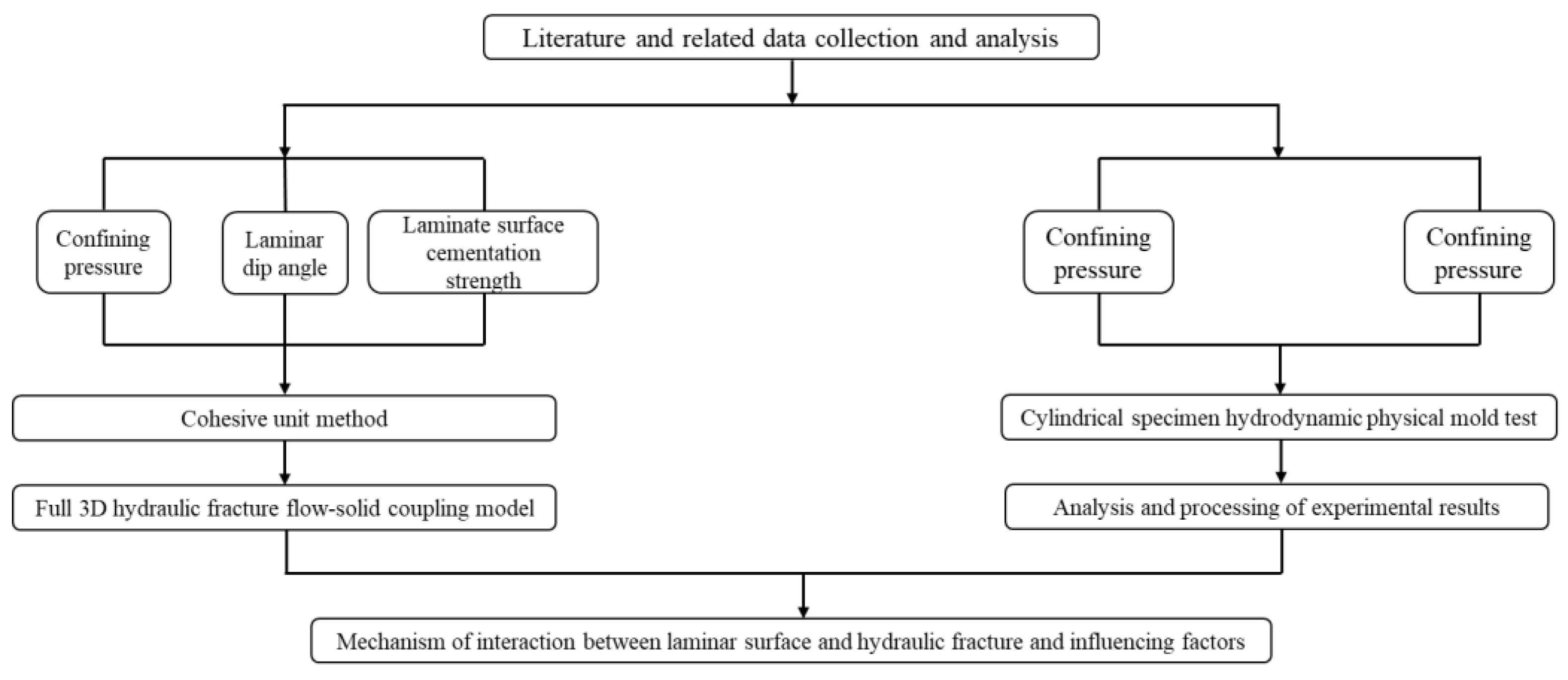
The study is carried out in two directions, numerical simulation and physical model testing, and the specific technology roadmap is shown in Figure 1.
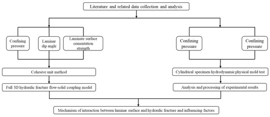
Figure 1.
Research roadmap.
There are currently three main techniques for simulating crack extension problems in Abaqus (Abaqus is a powerful suite of finite element software for engineering simulation, and its problem-solving capabilities range from relatively simple linear analysis to many complex nonlinear problems). Compared with the other two techniques, the cohesive unit used in this paper is a damage mechanics model using the traction–separation criterion, which can better deal with the singularity of the crack tip and, at the same time, can consider the intraseam fluid flow and is the most widely used crack extension technique.
2.1. Model Control Equations
2.1.1. Cohesive Pore Pressure Unit
- (1)
- Cohesive pore pressure unit introduction
In this paper, the cohesive unit with pore pressure is used to simulate the initiation and extension of hydraulic fractures and the laminar flow and filtration of fluid into the matrix inside the fracture. The cohesive unit has two main functions:
- ①
- To simulate hydraulic fracture initiation and extension based on the traction–separation criterion;
- ②
- To describe the tangential flow of the fluid within the fracture and the normal flow perpendicular to the wall.
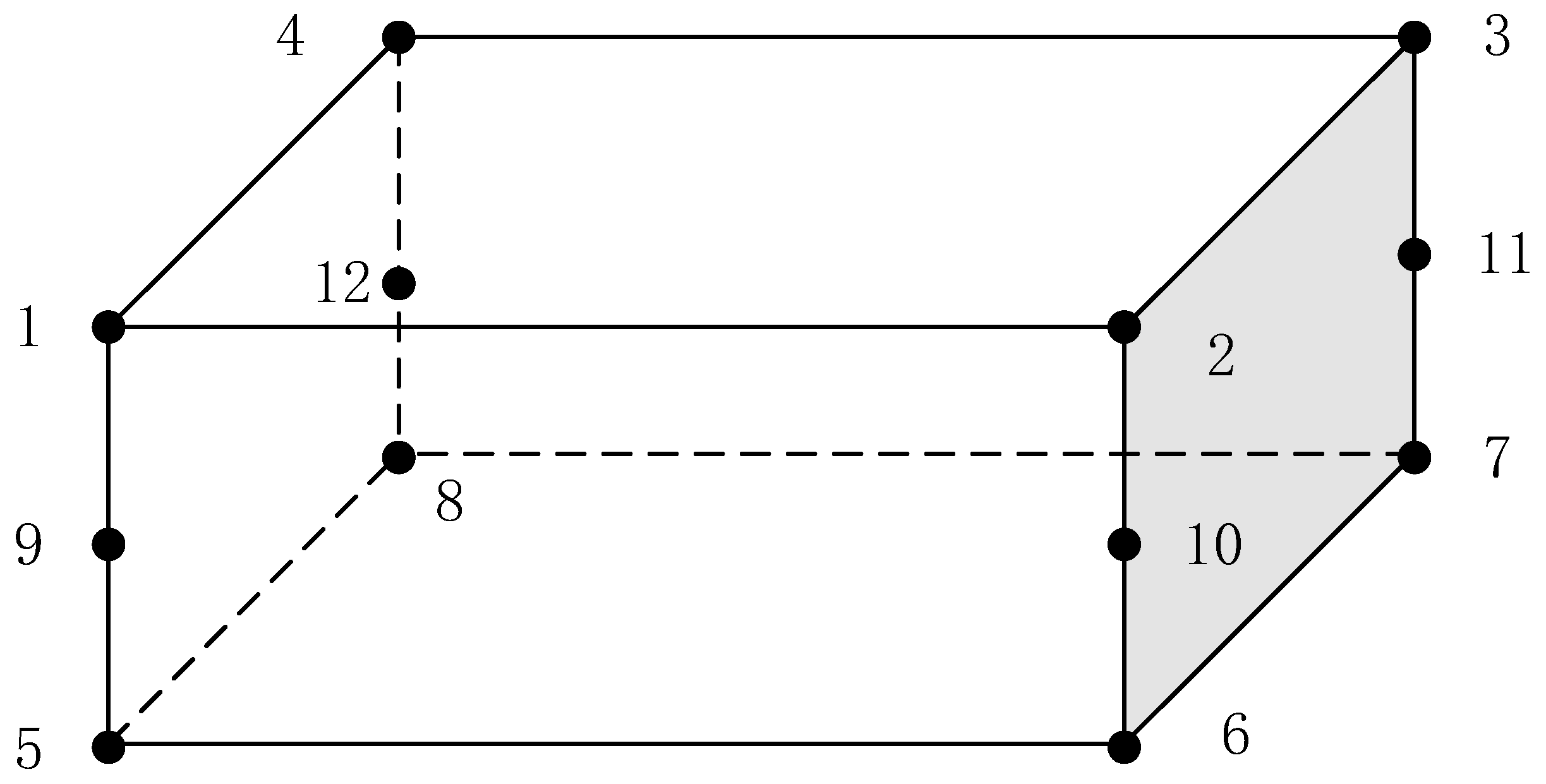
Figure 2 shows the distribution of the 12 nodes of the 3D hole pressure cohesive cell. Nodes 1, 2, 3, and 4 form the upper surface of the cell; nodes 5, 6, 7, and 8 form the lower surface of the cell; and nodes 9, 10, 11, and 12 are the pore pressure nodes.
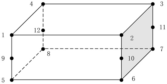
Figure 2.
Three−dimensional hole pressure cohesive cell.
The stress-strain relationship of the cohesive cell before damage occurs is consistent with the following linear elastic deformation:
where is the stress tensor of the cohesive cell and is dimensionless; is the normal stress of the cell, and the units are MPa; and are the tangential stresses of the unit, and the units are MPa; is the stiffness matrix of the cell and is dimensionless; and is the unit stress and is dimensionless.
When a cohesive unit is used to simulate material damage, its geometric thickness is generally defaulted to 0 before the simulation, while the concept of intrinsic thickness is introduced to replace the actual thickness of the unit to avoid singularities in the calculation, which is generally set to 1. Therefore, the displacement and strain of the cohesive unit are numerically equal.
- (2)
- Unit damage model
The damage mechanism of the cohesive unit follows the traction strain criterion, mainly based on the stress to which the unit is subjected as the basis for unit damage and failure. Before the damage of the unit, the displacement of the unit should be proportional to the stress. When the stress reaches the ultimate strength of the material, the unit begins to damage, the stress that can be withstood with the increase in displacement gradually decreases to zero, and then the unit fails.
Figure 3 shows a schematic diagram of the damage intrinsic model in the normal direction of the cohesive unit, and the other two tangential directions have the same damage mode mechanism. When the displacement normal to the unit is smaller than the initial damage displacement of the unit , with the increase in the displacement, the stress normal to the unit increases, and the unit at this stage shows the characteristics of linear elasticity and the specific characteristics controlled by the unit penalty stiffness . When the normal stress of the cohesive unit reaches the strength of the material , the unit begins to damage. With the increase in the normal displacement, the stress normal to the unit gradually decreases. In this stage, the cohesive unit shows the characteristics of softening. When the normal displacement reaches the displacement of the complete destruction of the unit , the unit bears the stress of 0, and the unit completely fails (in the figure, is the current strain before the damage to the stiffness of the obtained tension, Pa; is the material tensile strength, Pa; is the actual tensile stress, Pa; D is the damage factor; and , , and are the displacement of the completely destroyed unit, the maximum displacement during the loading process, and the displacement upon initial damage, respectively, m).
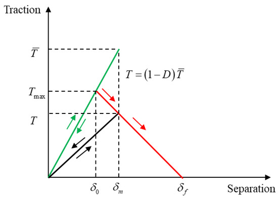
Figure 3.
T–S damage criterion for cohesive cells.
- (3)
- Initial cracking guidelines of the unit
- ①
- Maximum stress criterion
When the stress value in any one direction of the cohesive cell reaches the critical stress value, the cell starts to break:
where is the tensile strength of the rock, and the units are MPa; and are the shear strengths of the rock in the other two directions, and the units are MPa; and <> indicates that the unit is subjected to tensile stress damage only, and no damage occurs for compressive stress or compressive deformation units.
- ②
- Secondary stress criterion
The cohesive unit begins to break under the condition that the unit is subjected to stress in three directions, and its corresponding critical value of the square of the ratio is equal to 1:
where is the unit normal stress, and the units are Pa, and and are the critical stresses in the first all direction and second tangential direction of the cohesive unit, respectively, and the units are Pa.
- ③
- Maximum stress criterion
When the strain value in any direction of the cohesive cell reaches a critical value, the cell starts to break:
where is the critical strain normal to the rock and is dimensionless, and and are the critical strains in the other two directions of the rock and are dimensionless.
- ④
- Secondary strain guidelines
The cohesive cell begins to break under the condition that the sum of the squares of the strains in the three directions of the cell and its corresponding critical strain ratio is equal to 1:
In practice, cracks are generally a combination of two modes, tensile and shear, and in Abaqus, a mixed mode ratio of these two types is simulated in stress mode and energy mode, respectively.
- ⑤
- Hybrid mode based on the stress mode ratio
The mixed mode of fracture extension is defined by the relationship between the given total rupture displacement and the mixed mode ratio :
where and are the mixed−mode ratios and are dimensionless.
- ⑥
- Hybrid mode based on energy mode
The mixed−mode ratio using the energy mode definition is
where Gn is the work performed by the normal displacement of the cohesive cell, and the units are J; Gs and Gt are the work performed by the displacements in the remaining two directions of the cell, and the units are J.
- (4)
- Cohesive cell expansion guidelines
The cohesive cell uses stiffness degradation to describe the damage evolution process of the cell, and its expression is
The damage factor is calculated by the formula
- (5)
- Fluid flow equation in the unitary damage zone
The fluid flow in the damage area of the cohesive cell is divided into the flow along the tangential direction and the normal filtration loss perpendicular to the upper and lower surfaces of the cohesive cell, as shown in Figure 4.
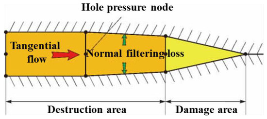
Figure 4.
Cohesive unit damage zone fluid flow diagram.
Assuming that the fluid inside the cohesive cell is an incompressible Newtonian fluid, the equation for its tangential flow is
where is the tangential flow rate in units of m3/s, is the pressure gradient along the length of the cohesive unit in units of Pa/m, and is the fracture width in units of m.
The normal filtration loss on the upper and lower surfaces of the cohesive cell can be described as
where and are the filtration loss coefficients of the upper and lower surfaces, respectively, and the units are m3/(Pa·s).
The equation for the conservation of fluid mass in the cohesive cell is
where is the fracturing fluid injection rate, and the units are m3/s.
2.1.2. Hole Pressure Unit Embedding Method
To study the fracture extension of the nodal developed formation, it is necessary to embed the cohesive pore pressure unit globally into the model and simulate the fracture extension behavior based on the damage cracking of the cohesive pore pressure unit. In this paper, the program to embed the global cohesive pore pressure unit is written using the Python language. The programming is based on the inp. file. First, the model inp. file information is read, all the units and unit node information are iterated, and the number of node occurrences is recorded. According to the number of node occurrences for node splitting to generate new nodes, the new nodes are assigned to each unit, and cohesive units are generated at the common edge of the unit. The new units, nodes, and cohesive unit are output. Then, the information of seepage nodes is created, and the seepage nodes are assigned to cohesive units to generate cohesive pore pressure units that support seepage. Finally, the newly generated inp. file is submitted to Abaqus for processing and analysis.
The cohesive pore pressure unit consists of information from six nodes. In addition to the basic four unit nodes, the unit should also contain two seepage nodes. The seepage nodes are located in the middle of the unit thickness direction, so the cohesive unit intersection shares the same seepage node, and it is necessary to use the node merging tool to merge the seepage nodes at the intersection location, as shown in Figure 5.
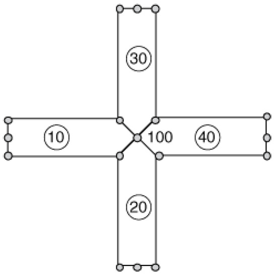
Figure 5.
Cohesive seepage node at the merged intersection location.
2.2. Benchmarking Example
Hydraulic fractures usually produce complex fracture morphologies when expanding in shale reservoirs, while weak surfaces such as shale laminae and natural fractures present in the shale oil reservoirs can have an important impact on the hydraulic fracture expansion behavior and the final fracture distribution characteristics during fracture modification. In this paper, the expansion process of hydraulic fractures in a reservoir is simulated by using the method of globally embedded cohesive units. The modeling process requires prespecifying the distribution location and morphological characteristics of the laminar joints, so the corresponding preprocessing script files are written in the Python language, and different types of laminar joints are flexibly arranged by the idea of parametric modeling. The computational model is shown in Figure 6. The model size is 20 × 20 m, and the injection point is located at the center of the model (i.e., (0,0)). Ten laminar surfaces are initially set, and each laminar surface is composed of several microlaminates with a length distribution of 2–4 m. The laminar joints are spaced at 1–2 m, and there are 37 laminar joints in the whole model. The laminated joints have no initial opening, the angle with the x-axis is 30°, the x-direction is the minimum horizontal principal stress direction, and the y-direction is the vertical principal stress direction.
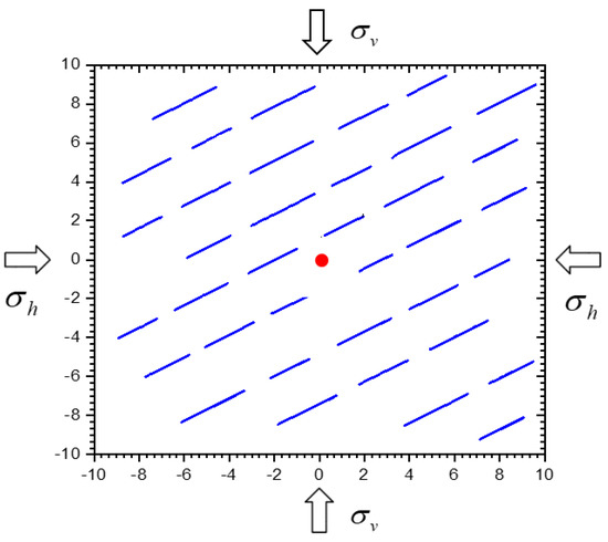
Figure 6.
Distribution of laminated joints and model forces.
The grid division is shown in Figure 7. The computation area is divided by a quadrilateral grid, the cell type is CPE4P, the cell size is approximately 0.2 m, and there are 59,612 nodes and 35,449 cells in the model, including 11,883 quadrilateral block cells and 23,566 cohesive cells. The cohesive cell type is COH2D4P. The outer boundary of the model is subjected to fixed displacement and impermeable boundary conditions, where the upper and lower boundaries constrain the displacement in the y-direction and the left and right boundaries constrain the displacement in the x-direction.
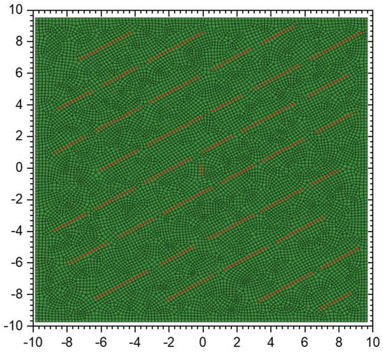
Figure 7.
Finite element meshing.
To analyze the effects of different parameters on the hydraulic fracture extension behavior, sensitivity analysis of each parameter is needed. Therefore, a set of parameters needs to be selected first as the benchmark case, and the subsequent sensitivity analysis is carried out by changing the corresponding parameters on this basis. The base parameters used in the benchmark case are shown in Table 1.

Table 1.
Model base input parameters.
In the benchmark case, the injection displacement is 0.002 m2/s, the injection duration is 20 s, the stress boundary condition is the effective stress, the difference between the overlying rock pressure and the minimum horizontal principal stress is 2 MPa, and the values in Table 1 are used for other parameters.
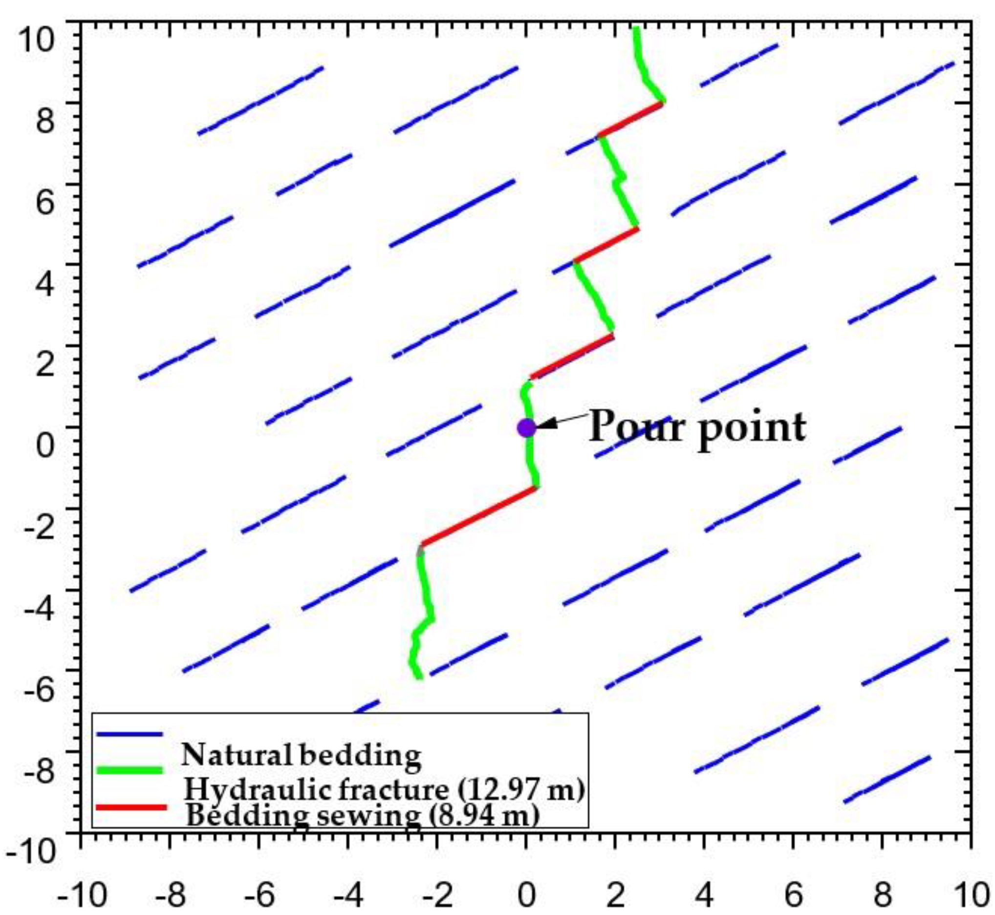
Figure 8 shows the fracture pattern at the end of injection. The blue dashed line represents the initial laminar fracture, the green dashed line represents the expansion path of the hydraulic fracture in the reservoir matrix, and the red dashed line indicates the activated laminar fracture.
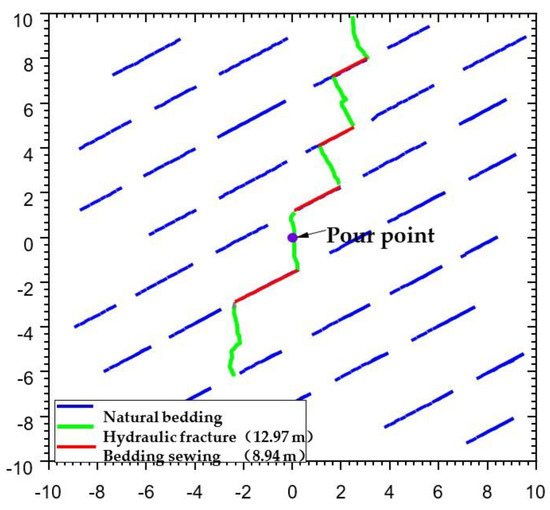
Figure 8.
Crack pattern at the end of injection.
After the hydraulic fracture starts to crack from the injection point, it expands along the direction perpendicular to the minimum horizontal principal stress. After encountering the first group of laminated joints, the hydraulic fracture turns along the laminated joints because the tensile strength of the laminated joints is lower than the tensile strength of the shale matrix, and when the hydraulic fracture continues to expand and meets the second group of laminated joints, the hydraulic fracture continues to expand along one side of the laminated joints. Meanwhile, on the other side of the laminated joints, it does not continue to expand, which is mainly because as the width of the hydraulic fracture increases, the stress state on both sides of the laminated joints on both sides of the intersection point is different, and the laminated surface on the right side of the intersection point tends to open in tension, while the laminated joints on the left side of the intersection point tend to close in compression. When the hydraulic fracture expands to the tip of the laminated joints, under the superposition of both the crack-tip-induced stress field and the far-field stress, the hydraulic fracture undergoes a certain deflection and re-expands in the direction perpendicular to the minimum horizontal principal stress. The intersection behavior of the hydraulic fracture and the laminar joints in the subsequent expansion process is similar to the above process. The total length of the fracture formed at the end moment of fluid injection is 21.91 m, among which the length of the activated lamina joints is 8.94 m and that of the formed hydraulic fracture is 12.97 m. Figure 9 shows the displacement field in the x-direction in the rock at the end moment of injection, from which it can be seen that the maximum seam width of the hydraulic fracture is approximately 1.1 mm, while the width of the lamina joints is significantly smaller than the width of the hydraulic fracture. In addition, in this calculation, the laminated seam not only occurs normal to the tension but also has a certain degree of shear deformation. The presence of laminated joints not only affects the expansion path of hydraulic cracks but also affects the fluid pressure inside the cracks.
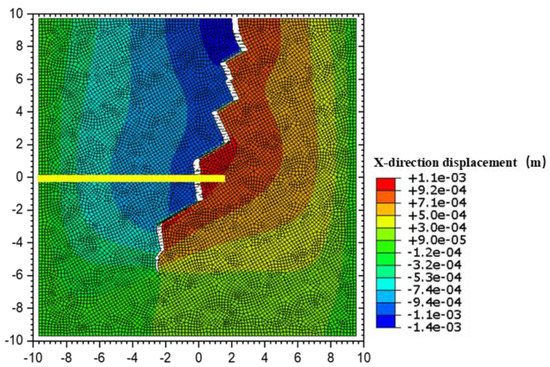
Figure 9.
Displacement in the x-direction at the end moment of injection (magnified 200 times).
2.3. The Effect of Differential Ground Stress
The magnitude and direction of the ground stress have an important influence on the expansion path and final morphology of the hydraulic fractures. For this reason, this subsection mainly analyzes the interaction mechanism between laminated joints and hydraulic fractures under different horizontal ground stress difference conditions (0, 2, and 6 MPa), and other parameters are the same as those in the benchmark calculations.
Figure 10 shows the morphology of the seam network at the end of injection under a uniform horizontal ground stress. When the hydraulic fracture expands to the tip of the laminated seam, it continues to expand along the direction of the laminated seam.
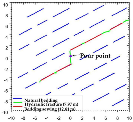
Figure 10.
Crack pattern at the end of injection when the ground stress difference is 0 MPa.
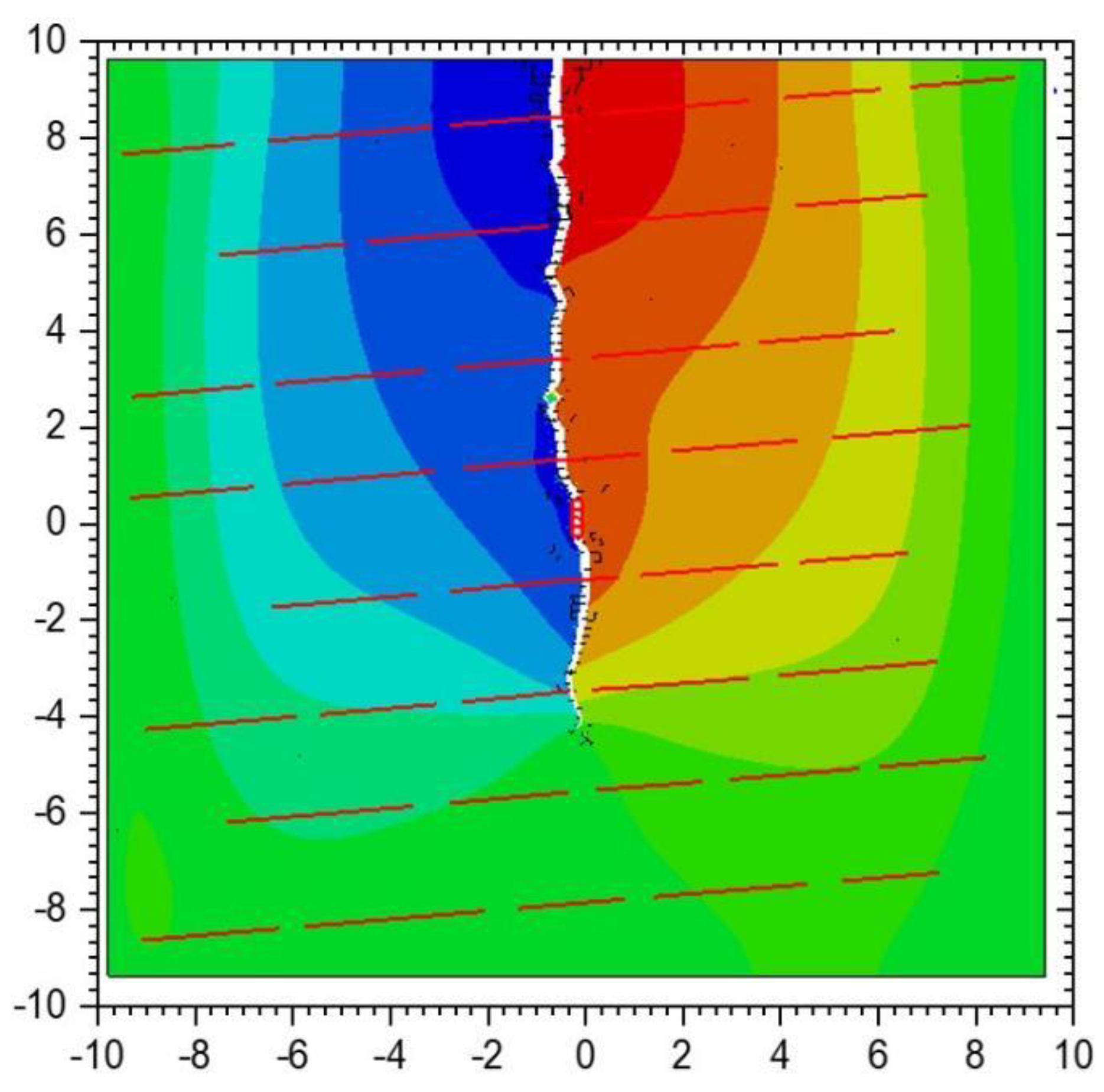
Figure 11 and Figure 12 show the geometry of the seam network formed when the ground stress difference is 2 and 6 MPa, respectively. Compared with the case where the difference in ground stress is 0 MPa, the hydraulic fractures still expand in the direction perpendicular to the minimum horizontal principal stress after intersecting with the laminae. When the difference between the overlying rock pressure and the minimum horizontal principal stress increases to 6 MPa, it can be seen that the hydraulic fractures tend to pass directly through the laminae joints, resulting in a decrease in the number of activated laminae joints. This is mainly because the greater the difference in ground stress is, the greater is the value of positive stress on the laminated joints, and the less likely they are to be activated.
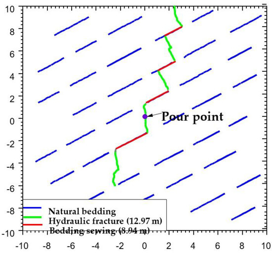
Figure 11.
Crack pattern at the end of injection when the ground stress difference is 2 MPa.
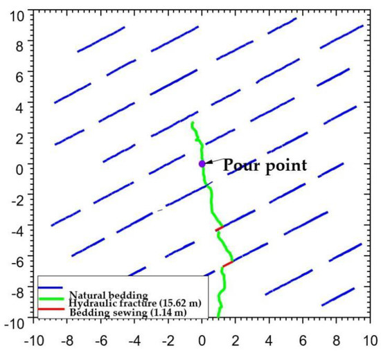
Figure 12.
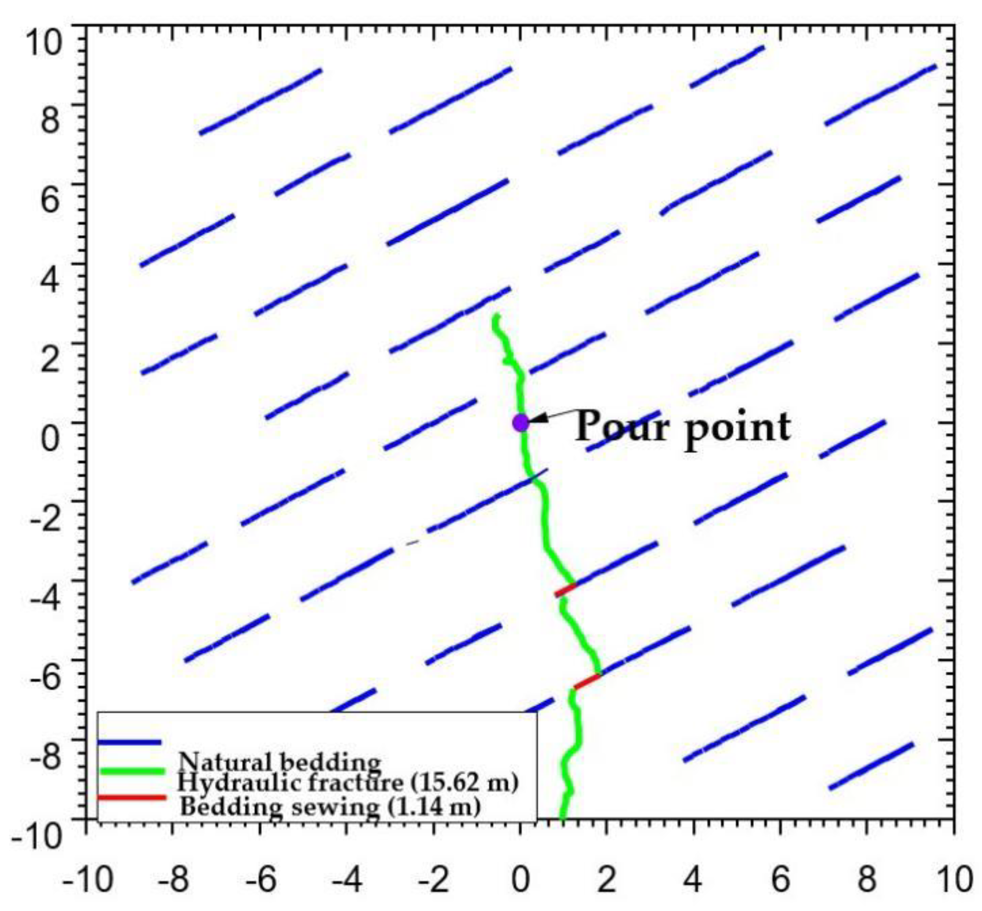
Crack pattern at the end of injection when the ground stress difference is 6 MPa.
The crack lengths formed under different ground stress difference conditions were counted. The total crack length increased from 20.58 to 21.91 m as the ground stress difference increased from 0 to 2 MPa, but the total length of hydraulic cracks in the former was 7.97 m and the total length of laminated joints was 12.61 m, while the total length of hydraulic cracks in the latter was 12.97 m and the total length of laminated joints was 8.94 m. After the ground stress difference increased to 6 MPa, the total crack length was 16.76 m, among which the total length of hydraulic cracks was 15.62 m and the total length of laminar joints was 1.14 m. The above calculation results show that the existence of a certain ground stress difference is beneficial to communicate more laminar joints and form a more complex crack network, while an excessively large ground stress difference will reduce the complexity of artificial cracks.
2.4. Effect of Laminar Dip Angle
This subsection focuses on the influence law of the hydraulic fracture extension path and final morphology for different laminar surface inclination angles (5°, 30°, and 60°), and the other parameters are the same as those in the baseline calculation.
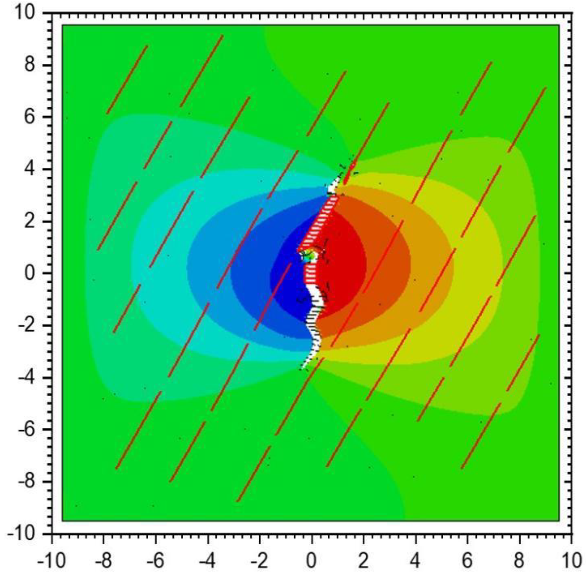
Figure 13 shows the crack expansion pattern at the end of injection when the laminated seam inclination angle is 5°. The figure shows that the hydraulic fracture expands along the direction perpendicular to the minimum horizontal ground stress after starting from the injection point, and the hydraulic fracture tends to continue to expand directly through the laminated seam after meeting the laminated seam.

Figure 13.
Crack pattern at the end of injection with a laminar seam dip angle of 5°.
Figure 14 and Figure 15 show the morphology of the seam network when the laminar seam dip angle is 30° and 60°, respectively, and it can be seen from the figures that as the laminar seam dip angle increases, the hydraulic fractures are more likely to turn and expand along the laminar direction.
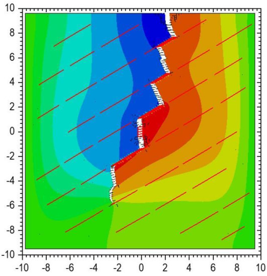
Figure 14.
Fracture morphology at the end of injection when the dip angle of the bedding fracture is 30°.

Figure 15.
Fracture morphology at the end of injection when the dip angle of the bedding fracture is 60°.
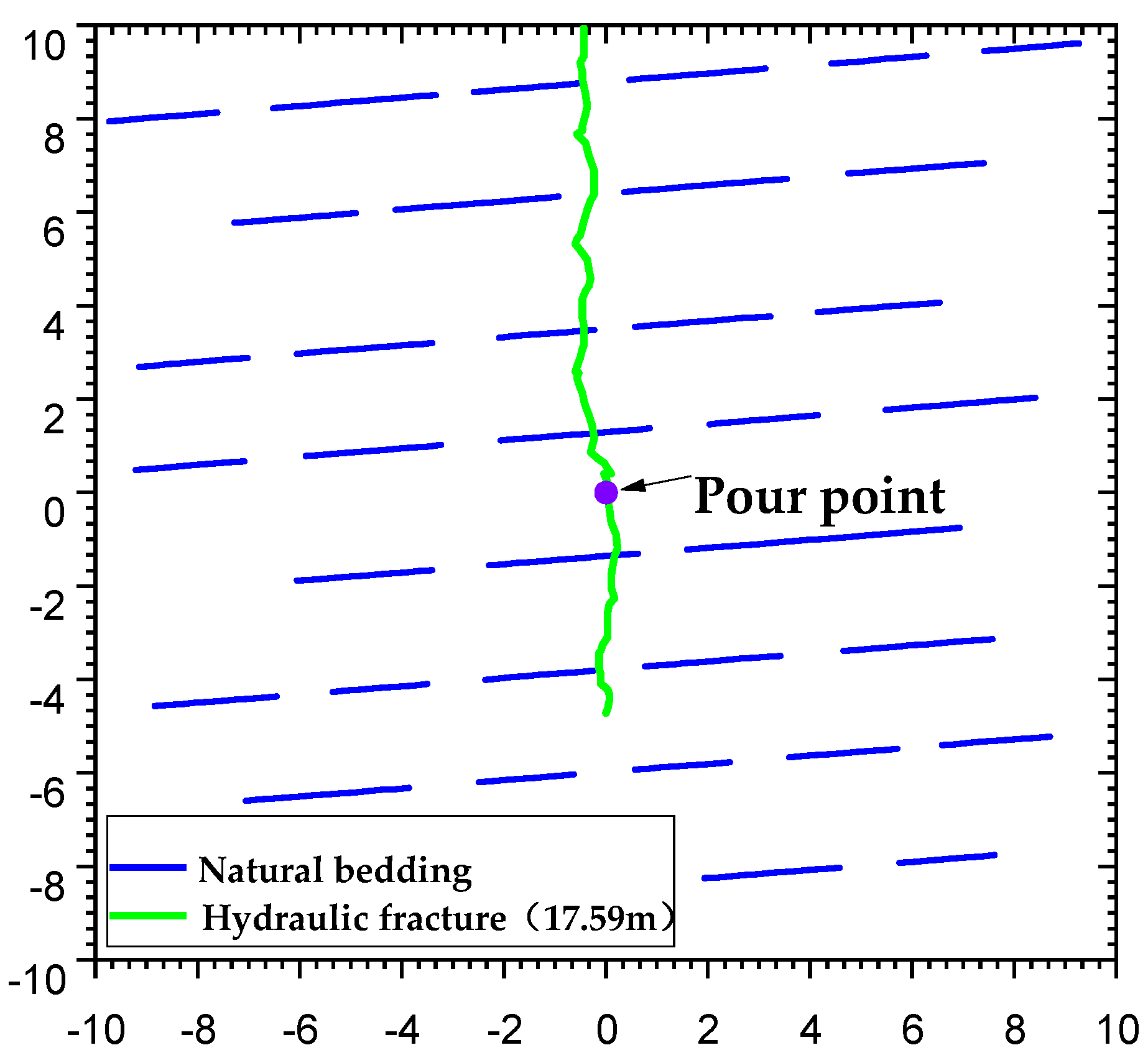
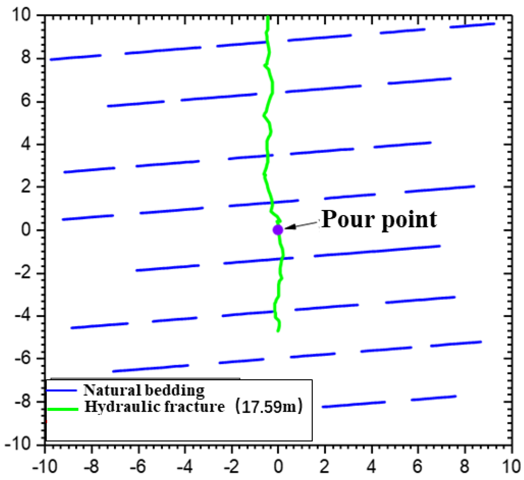
Figure 16 and Figure 17 show the morphology of the seam network when the laminated seam inclination angle is 5° and 30°, respectively, from which it can be seen that when the laminated seam inclination angle is 5°, the total length of the artificial fracture is 17.59 m, and the laminated seam is not activated; when the laminated seam inclination angle is 30°, the total length of the artificial fracture is 21.91 m, of which the laminated seam opening length is 8.94 m. This is mainly because when the inclination angle of the laminated joints is small, the positive stress value acting on the wall of the laminated joints is larger, and the hydraulic fracture tends to continue to expand along the original path directly through the laminated joints. It can be seen that as the dip angle of the formation is larger at the location of the back−sloping slope, a complex fracture network is more likely to be formed after hydraulic fracturing.
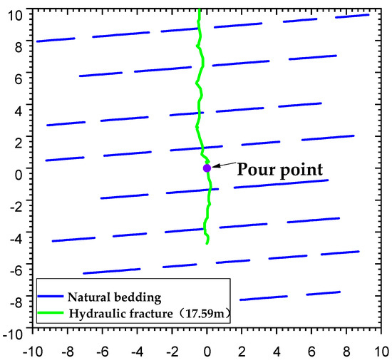
Figure 16.
Fracture morphology at the end of injection when the bedding dip angle is 5°.
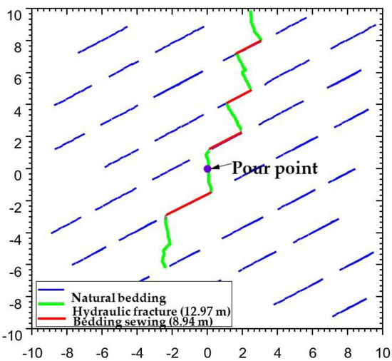
Figure 17.
Fracture morphology at the end of injection when the bedding dip angle is 30°.
2.5. Effect of Laminar Cementation Strength
The laminar tensile and shear strengths also have an important influence on the expansion pattern of hydraulic cracks, and this section focuses on the influence of laminar tensile strength on the expansion path and final pattern of hydraulic cracks.
Figure 18 shows the crack expansion pattern at the end of injection when the laminated seam inclination angle is 5° and the laminated cementation strength is 2 MPa. From the figure, it can be seen that the hydraulic cracks expand along the direction perpendicular to the minimum horizontal ground stress after starting from the injection point, and the hydraulic cracks tend to expand directly through the laminated seam after meeting the laminated seam.
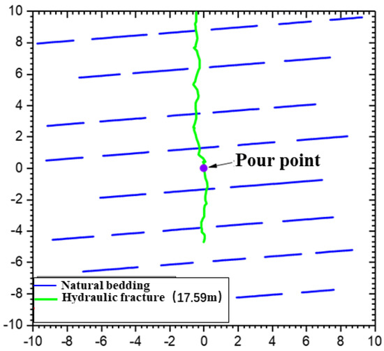
Figure 18.
Crack pattern at the end of injection when the laminar tensile strength is 2 MPa.
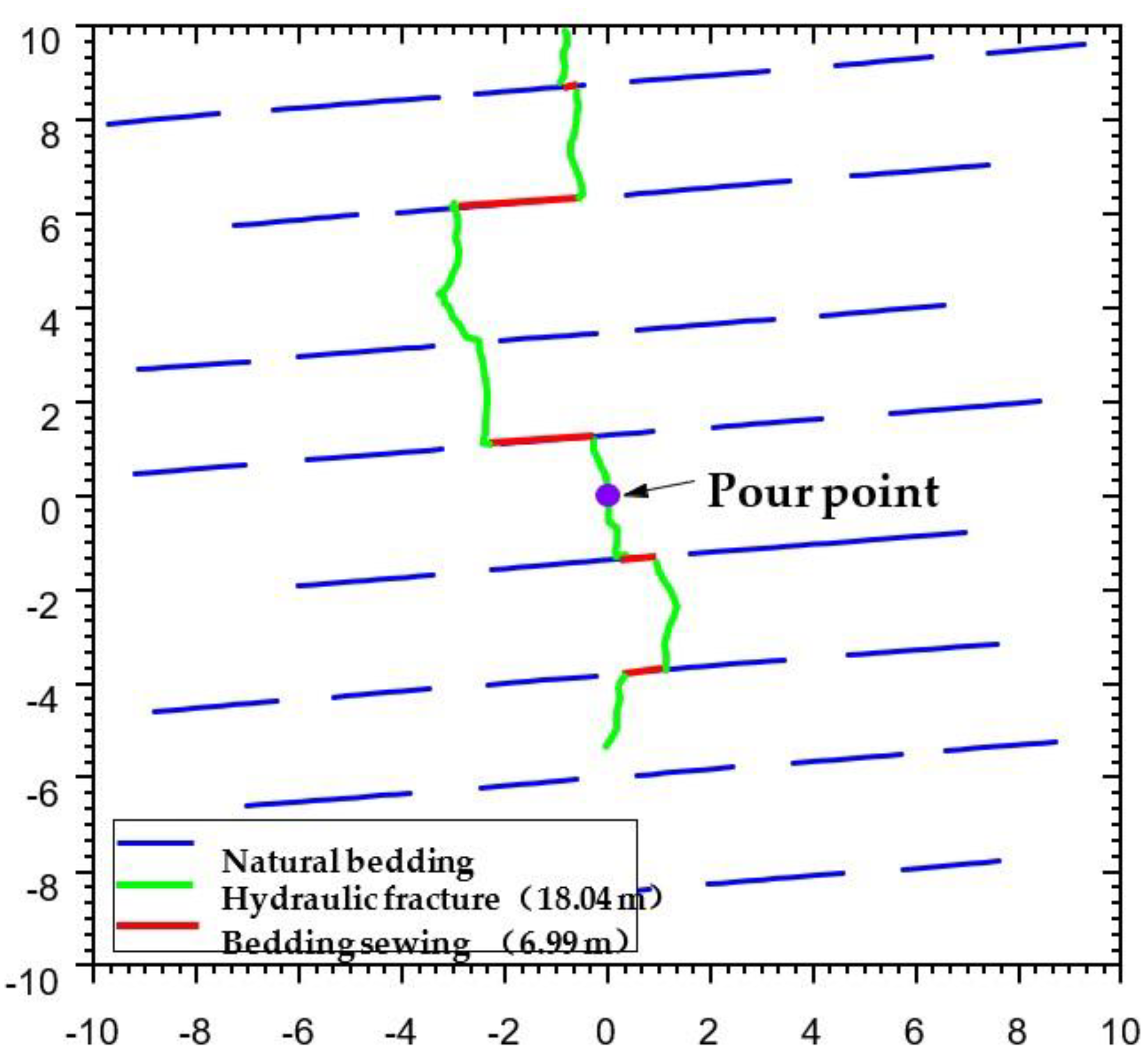
Figure 19 shows the crack expansion pattern at the end of injection when the laminated seam inclination angle is 5° and the laminated cementation strength is 0.5 MPa. From the figure, it can be seen that the hydraulic crack meets the laminated seam and then expands along the laminate, and after the hydraulic crack expands to the tip of the first level of the laminated seam, it turns to the direction perpendicular to the maximum ground stress and continues to expand and still turns when it meets the next level of the laminated seam. The total length of artificial cracks is 25.03 m, among which the total length of hydraulic cracks is 18.04 m and the total length of laminated joints is 6.99 m. It can be seen that under the same combined state of ground stress and the same dip angle of the laminated surface, the lower the tensile strength of the laminated surface is, the more likely the hydraulic cracks induce shear slip of the laminated surface, and the complexity of cracks increases significantly.
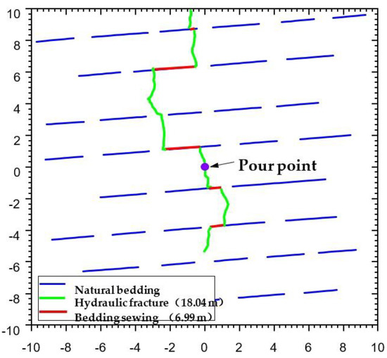
Figure 19.
Crack pattern at the end of injection when the laminar tensile strength is 0.5 MPa.
3. Hydraulic Fracturing Experiment
To ensure the accuracy of the numerical simulation results and the applicability of practical engineering, an indoor physical simulation experiment of hydraulic fracturing was carried out with an outcrop of marine shale of the Longmaxi Formation in Wulong, Chongqing, under corresponding conditions. The acoustic emission test results and core section analysis were used to reveal the influence of ground stress, fracturing fluid discharge, viscosity, and other parameters on the multiscale fracture mechanism of shale.
3.1. Experimental Setup
In order to meet the needs of physical simulation experiments for fracturing shale cylindrical specimens, a physical simulation test system for fracturing shale cylindrical specimens was constructed in this study using a conventional triaxial rock mechanics experimental machine, and the overall structure is shown in Figure 20. The test system is mainly composed of a rock stress servo loading system, fracturing fluid injection system, and acoustic emission detection system. Among them, the rock stress servo loading system is mainly used to provide the stress state of the deep shale and simulate the real stress environment of the formation. The fracturing fluid injection system is mainly used to inject fracturing fluid into the specimen simulation wellbore with constant pressure/flow rate and realize the real−time acquisition of pump pressure and discharge volume. The acoustic emission detection system is mainly used to detect the microfracture signal during the shale hydraulic fracturing process and obtain the real−time hydraulic fracture initiation and spatial distribution characteristics.
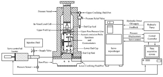
Figure 20.
Shale cylindrical specimen fracturing physical simulation test system.
- (1)
- Rock stress servo loading system
The rock stress servo loading system is mainly composed of a fully digital electrohydraulic servo rock triaxial test system produced by Beijing Zhongchuang Test Instrument Technology Co. The system mainly includes: a rock core high−pressure triaxial chamber, servo hydraulic source, servo booster, portal rigid frame, radial/axial strain gauge, heating system, and digital acquisition system, and so on. The system has a maximum output axial force of 2000 kN and a maximum working circumferential pressure of 140 MPa, which can better meet the requirements of stress size for deep shale fracturing; meanwhile, it is equipped with a specimen heating and constant temperature system with an upper limit temperature of 100 °C. The maximum allowable specimen size is Φ100 mm × 200 mm, and it is equipped with an axial/radial strain gauge with 0.0001 mm resolution and 0.3% measurement accuracy.
- (2)
- Fracturing fluid pumping system
The fracturing fluid pumping system is mainly used to provide a constant flow of high-pressure fracturing fluid. In order to provide a more accurate flow control than most reciprocating pumps, this test system uses a Teledyne Isco 260HP high-precision high-pressure plunger pump as the power source of fracturing fluid (Figure 21), leakage of 0.50 μL/min, maximum output pressure of 65.5 MPa, measurement accuracy of 0.1%, and equipment operating temperature of 5–40 °C.
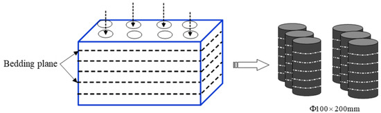
Figure 21.
Schematic diagram of the processing flow of cylindrical specimens.
- (3)
- Acoustic emission detection system
The acoustic emission detection system is mainly composed of five modules: host, sensor, preamplifier, acquisition card, and AEWin signal acquisition and analysis software, as shown in Figure 22. The selection of an acoustic emission sensor has an important impact on the detection results. The acoustic emission probe selected in this test is the SR40M-type low-frequency narrow-bandwidth probe produced by Beijing Shenghua Xingye Technology Co. (Beijing, China). Because the acoustic emission sensor has high output impedance and weak output current, it is not suitable for long-distance transmission, so it needs to connect a preamplifier to amplify the voltage signal of the sensor several times before outputting to the acquisition card. The acoustic emission preamplifier used in this test is a 2/4/6-type amplifier manufactured by Physical Acoustics Corporation (PAC), with an adjustable gain of 20, 40, and 60 dB. The core component of the acoustic emission detection system consists of eight PCI-2 acoustic emission acquisition cards, a high-performance/low-cost acoustic emission acquisition card developed by PAC for research institutions with a built-in 40 MHz, 18-bit A/D converter for real-time analysis of samples, and higher signal processing accuracy with a minimum noise threshold of 17 dB. In addition, the PCI-2 system has a unique waveform stream data storage function, which can continuously store the acoustic emission waveform to the hard disk at a rate of 10 M per second. During the test, a layer of acoustic coupling agent is applied on top of the acoustic emission probe to ensure a tight bond between the probe and the specimen surface.
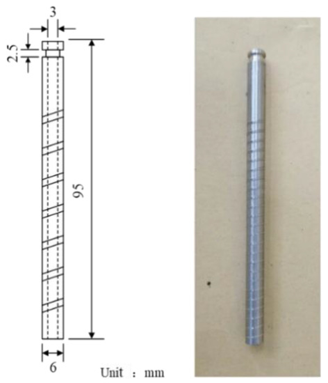
Figure 22.
Simulated casing geometry and physical drawing.
- (4)
- Industrial CT scanning system
Industrial CT (ICT) is an industrial application of computed tomography technology, which is mainly used for nondestructive testing and flaw detection of industrial products. ICT technology can closely and accurately reproduce the three-dimensional structure inside the object, and can quantitatively characterize the location, size, density variation, and level of defects inside the specimen. In this test, the Phoenix 300 kV/500 W all-purpose X-ray microfocus CT system manufactured by General Electric Company (GE) was used to observe and analyze the spatial spreading characteristics of hydraulic cracks in some postpressure specimens. The performance parameters of this CT test system are as follows: Phoenix v|tome|x m is the only micron CT system with breakthrough scatter|correct scattering correction technology introduced by GE for worldwide application. The system is equipped with a new-generation dynamic 41 detector, supporting a 2–3× CT scan speed or double CT resolution, maximum operating voltage of 300 kV, measurement accuracy of up to 4 + L/100 μm, maximum specimen size of 500 mm in diameter and 600 mm in height, maximum 3D scan area of 290 mm in diameter and 400 mm in height, maximum specimen weight of 50 kg, and maximum imaging pixels of 4048 × 4048 (16 M pixels).
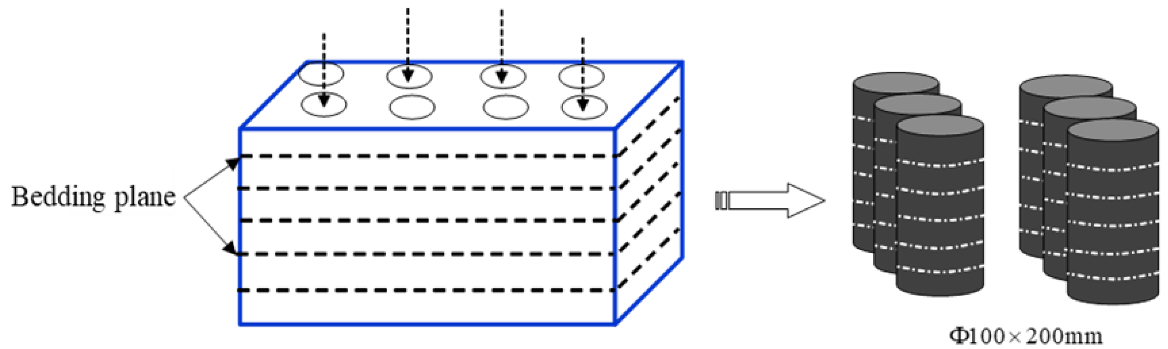
3.2. Specimen Preparation
The specimens used in this test are marine shale outcrops of the Longmaxi Formation, Shiqiao Township, Jiangkou Township, Wulong District, Chongqing, China. According to the requirements of the fracturing physical mode experiment of shale cylindrical specimens, 40 cylindrical specimens of Φ100 mm × 200 mm were drilled in the vertical lamina direction, and the upper and lower sections of the specimens were polished by a core end smoothing machine to ensure that the parallelism of the upper and lower surfaces was controlled within ±0.02 mm. The processing flow of the cylindrical specimens is shown in Figure 21.
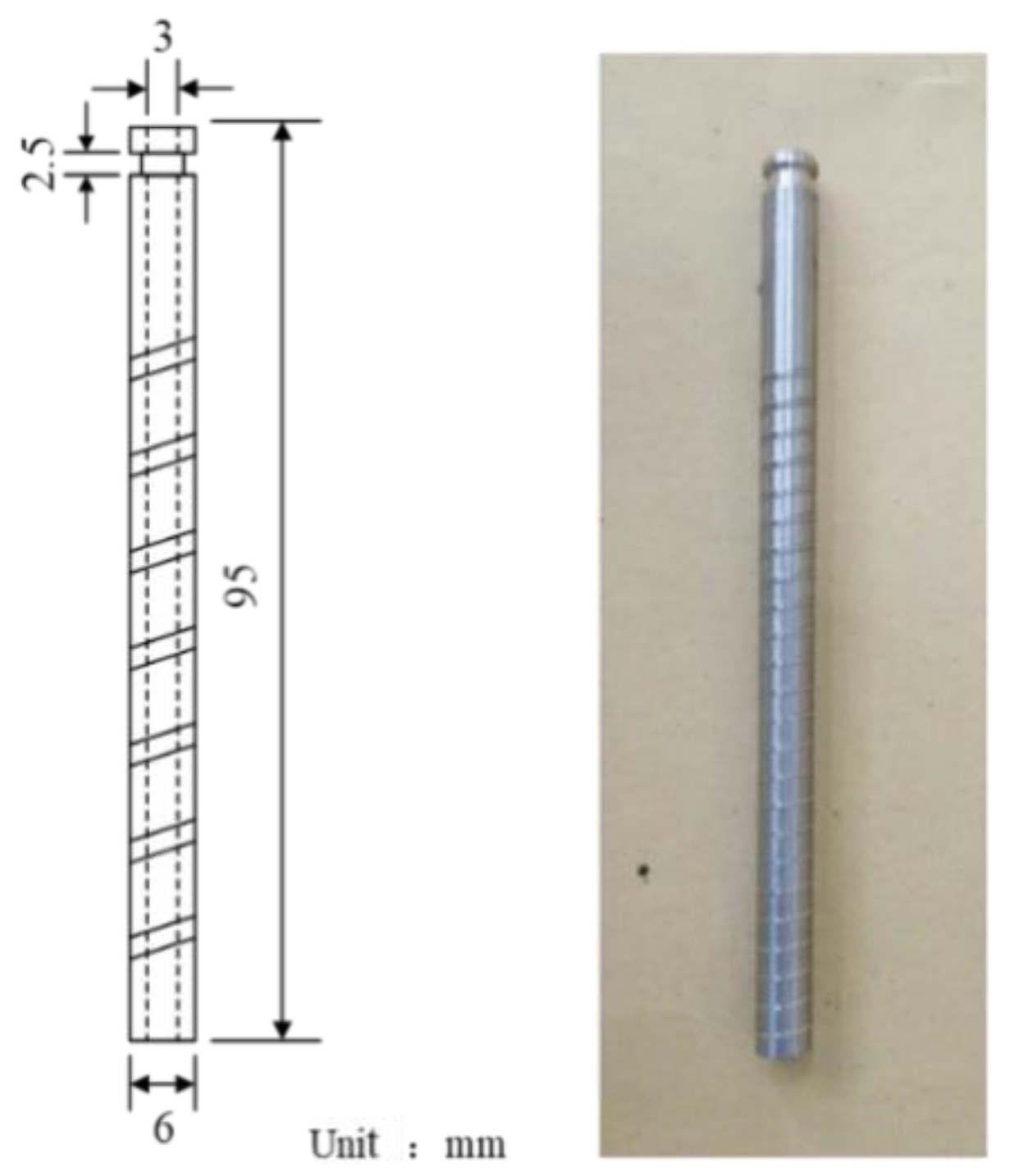
According to the design requirements of the simulation experiment, a simulated borehole with a diameter of 12.0 mm and a depth of 113.5 mm was drilled in the center of the cylindrical specimen, and a section of stainless steel tubing with an outer diameter of 6.0 mm, a wall thickness of 1.5 mm, and a length of 95.0 mm was buried as the simulated casing. Kraft K-9741 epoxy resin potting adhesive was used to seal the casing to the wellbore. To ensure sufficient bonding strength between the simulated casing and the wellbore, a rotary thread was machined on the outer surface of the simulated casing to increase the contact area between the casing and the glue; meanwhile, a ring-fitted recess was machined on the top of the casing to allow sealing treatment through a high-strength rubber seal. The dimensions of the simulated casing and the physical object are shown in Figure 22.
The processed shale cylindrical specimen is shown in Figure 23. A 27.0 mm long bare-eye section was reserved below the wellbore as the fracture initiation location. At the same time, the placement of the acoustic emission probe was marked on the outer surface of the specimen with “十”.
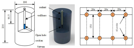
Figure 23.
Schematic diagram of the complete specimen and the placement of the acoustic emission probe.
To effectively monitor the microfracture signals in the shale hydraulic fracturing process, a total of eight acoustic emission probes were used in the experimental process of this paper, with four probes placed at the top and bottom of the cylindrical specimen. The specific parameters and arrangement positions are shown in Table 2.
Table 2.
Acoustic emission probe arrangement location and parameters.
3.3. Experimental Parameter Design
In this experiment, the controlled variable method was used to focus on the degree of influence of the absolute value of ground stress, fracturing fluid discharge, and viscosity on the hydraulic fracture expansion pattern of deep shale. Since it is difficult to simulate the real hydraulic conditions of the actual shale reservoir in the indoor hydraulic physical model test, the conditions of the shale hydraulic fracturing physical simulation experiment were determined by establishing similar criteria and referring to the actual ground stress magnitude and rock mechanics parameters of the shale to improve the credibility and reliability of the experiment. A total of 20 sets of cylindrical specimens were used for this experiment, among which a total of 4 sets of samples gave ideal experimental results, and the specimen numbers and testing conditions are shown in Table 3.
Table 3.
Hydraulic pressure physical simulation test scheme and results.
3.4. Experimental Procedure
This experiment uses multiple sets of equipment to work in concert, and the specific experimental steps are as follows:
- Prepressure description: The specimen laminae and natural fracture development are observed by the naked eye, and the location of the distribution of the weak surface of the primary structure is marked with a chalk or a marker.
- Gas tightness check: Since the shale laminae are more developed, shear misalignment is very likely to occur during specimen preparation, causing damage to the wellbore seal. Therefore, a certain amount of fluid is first pumped into the wellbore before the experiment, the pressure is maintained at approximately 0.5 MPa for 3–5 min, and the outer surface of the specimen is observed for the fracturing fluid oozing out.
- Acoustic emission probe installation: Eight acoustic emission probes are installed on the surface of the specimen, and a coupling agent is used to adhere the probes closely to the specimen while gently tapping each probe to ensure that each probe is working properly.
- Stress loading: The specimen is placed in the triaxial high-pressure chamber. The circumferential and axial pressures are loaded to the specified values in turn, and they are maintained for 10–20 min to ensure uniform stresses inside the specimen.
- Fracturing fluid injection: The Isco plunger pump is started, fracturing fluid is injected into the specimen according to the set displacement, acoustic emission detection is carried out simultaneously, the plunger pump and acoustic emission detection system are turned off when there is a significant drop in the pump pressure, and the axial pressure and circumferential pressure are unloaded in turn.
- Postpressure description: After the test, the surface of the specimen is first photographed by a digital camera to record the cracks on the surface of the specimen. Then, some specimens are selected to carry out a postpressure CT sweep to quantitatively characterize the spatial distribution of the hydraulic cracks. Finally, the post-test sample is cut to trace the hydraulic crack direction by a tracer display to summarize the hydraulic crack expansion law.
3.5. Experimental Results
3.5.1. Horizontal Ground Stress Difference
The experiment was set up with two horizontal ground stress differences of 3 and 6 MPa, and the surrounding pressure was 25 MPa. Using the hydraulic fracturing physical simulation test system, the fracturing fluid (slick water) was injected into the interior of the shale cylindrical core through the central hole at a constant discharge rate of 0.02 mL/s; the specific experimental results are shown in Table 4.
Table 4.
Experimental results of the effect of different horizontal differential stress conditions on hydraulic fracturing.
The native filling joints in the W–11 specimen were very developed (marked by blue lines in the Figure 24), and the experiments were conducted by applying 25 MPa of circumferential pressure and 3 MPa of shaft pressure and injecting slick water into the wellbore at a constant rate of 0.02 mL/s. It can be found through the experiments that after the pump pressure exceeded 1 MPa, the pump pressure increased linearly with time, and when the pump pressure rose to 51.36 MPa, the pump pressure dropped steeply, and the rupture was instantly detected. A large amount of acoustic emission time and high-amplitude acoustic emission energy were detected instantaneously, and the differential stress between the pump pressure and the surrounding pressure was 26.36 MPa at this time. The native filling fractures in the shale were partially opened after the pressure, and part of the native fractures were not only completely opened but also expanded to some extent. There are still two types of hydraulic fractures: one is two hydraulic fractures roughly symmetrical along the borehole axis, and the other is a laminated seam perpendicular to the borehole axis. Two of the three laminated seams are not fully extended through, and one laminated seam crosses the entire core.
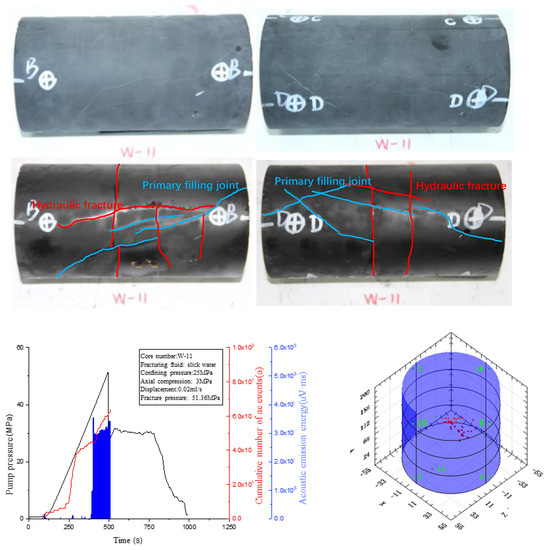
Figure 24.
W–11 triaxial condition hydraulic fracturing pumping curve and acoustic emission localization.
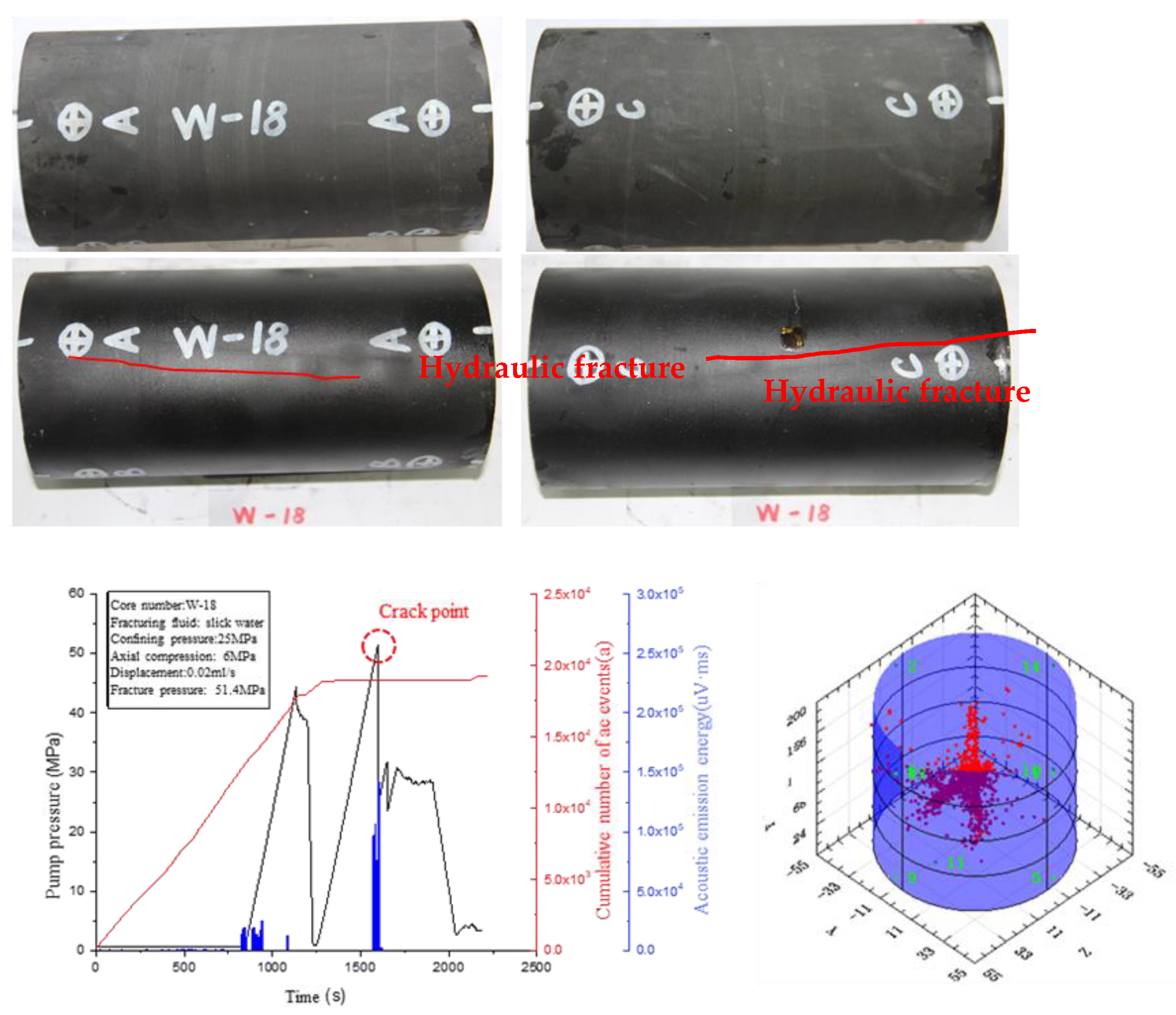
The perimeter pressure was maintained at 25 MPa, and the discharge rate was unchanged at 0.02 mL/s. The shaft pressure was increased to 6 MPa, and slick water was injected into the W–18 rock sample wellbore at a constant discharge rate. The photograph of the specimen W–18 after the test and the pumping pressure curve are shown in Figure 25. The rupture pressure was 51.4 MPa, which was almost the same as the rupture pressure of W–11 (i.e., 51.36 MPa). After observing the fractured rock sample, only two symmetrical and roughly axially oriented hydraulic seams were visible, and no laminar seams were formed.
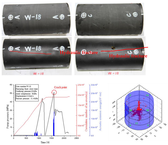
Figure 25.
W–18 triaxial condition hydraulic fracturing pumping curve and acoustic emission positioning.
By comparing W–11 and W–18, it can be seen that the rupture pressure only increases from 51.36 to 51.40 MPa under a circumferential pressure of 25 MPa when increasing the horizontal ground stress difference from 3 to 6 MPa, an increase of approximately 1.23%, which shows that under high circumferential pressure, the change in the horizontal stress difference stress (the difference between the overlying rock pressure and the horizontal ground stress) has a weaker effect on the shale rupture pressure. The effect of the change in the horizontal stress differential stress (the difference between the overlying rock pressure and the horizontal formation stress) on the shale rupture pressure is weakened. However, by comparing the fracture test results of W–11 and W–18 with the photographs before and after the test, it can be seen that with the increase in the horizontal ground stress difference, the difference coefficient of the vertical ground stress increases, the probability of longitudinal penetration of fractures along the maximum principal stress increases, the communicating horizontal laminated joints decrease, and the complexity of the fracture network decreases, so the experimental results of this control group are consistent with the numerical simulation results.
3.5.2. Laminar Dip Angle
Using the hydraulic fracturing physical simulation experiment system, based on previous experiments, we set the shaft pressure at 3 MPa, the surrounding pressure at 25 MPa, and the injection rate at 0.02 mL/s and conducted hydraulic fracturing physical simulation experiments on shale rock samples with lamina angles of 30° and 60° to analyze the relationship between the lamina face angle and hydraulic fracture formation and expansion. The experimental design and specific parameters are shown in Table 5.
Table 5.
Experimental results of hydraulic fracturing under different lamina angle conditions.
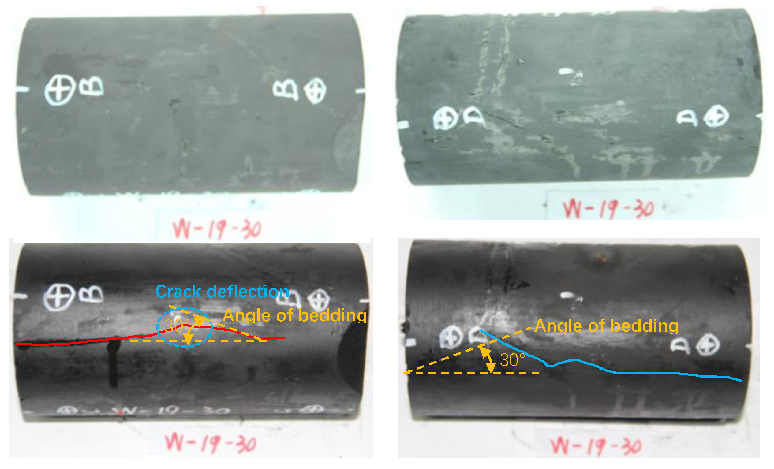
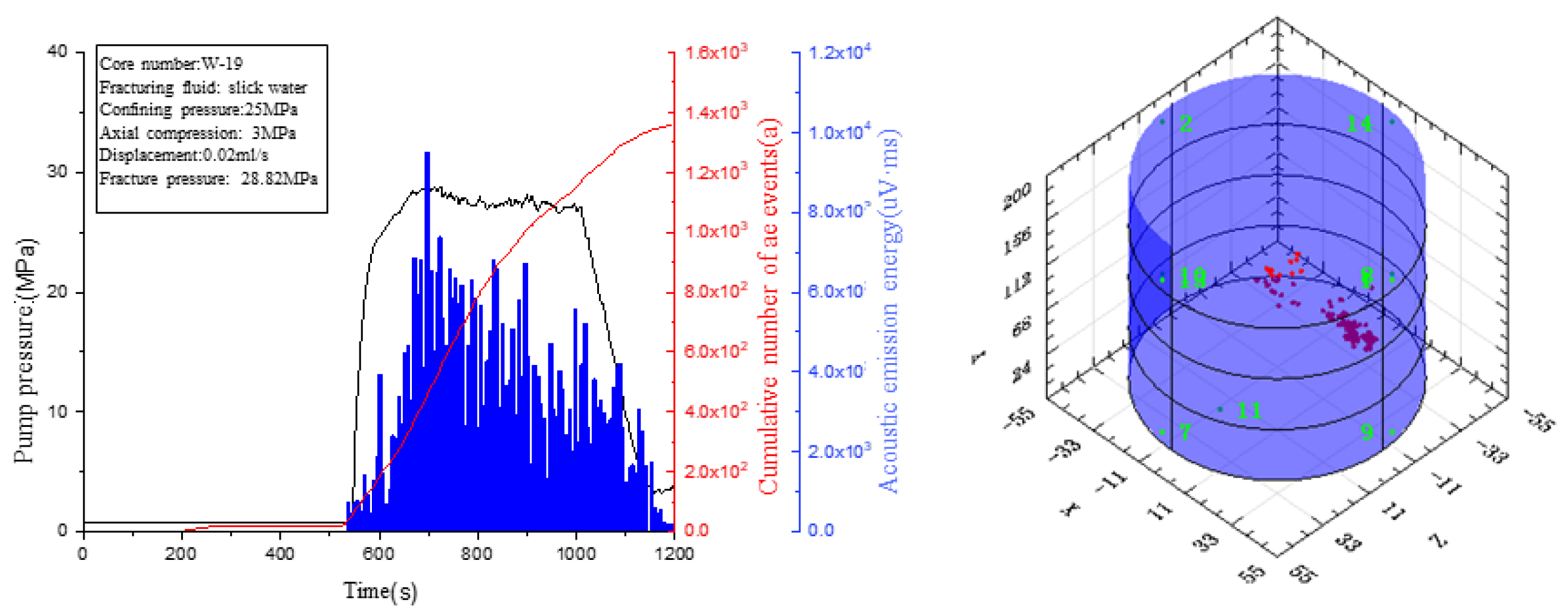
The W–19 rock sample was drilled at an angle of 30° to the parallel laminae direction, and a laminae seam with an approximately 30° angle to the borehole axis was visible near the buried pipe end before the experiment, in addition to a fracture along roughly the borehole axis and intersecting the laminae seam. After the experiment, the laminated seam intersected the borehole obliquely, the initial axially oriented fracture connected to it was opened, and a newly formed hydraulic fracture was present on the symmetrical side of the core. The photograph of the specimen W–19 after the test and the pumping pressure curve are shown in Figure 26. Eventually, a mixed-type seam network with hydraulic seams, laminar seams, and primary fractures opened simultaneously. From the pump pressure curve, the pump pressure first showed a linear increasing trend with time, and then the slope of the pump pressure increase slowly decreased, indicating the formation of new fractures in the core, and no obvious drop was observed in the pump pressure curve, which was mainly due to the influence of the primary fractures. The seam opening was larger, the high-pressure fluid inside the triaxial chamber after the fracture opening rapidly entered the interior of the core, and the pressure between the wellbore and the triaxial chamber was basically balanced, resulting in no steep drop in pressure. The pressure between the wellbore and the triaxial chamber was basically balanced, resulting in no steep pressure drop. The rupture pressure is 28.82 MPa, which is only 3.82 MPa higher than the surrounding pressure, and the rupture pressure of the rock is greatly reduced due to the influence of the weak structural surface. In addition, it can be observed that when a certain angle exists between the coring direction and the laminae, the fracture along the axial direction of the borehole will roughly deflect to the laminae direction to a certain extent, and when the fracture deflects and expands to a certain length, the fracture will return to the direction of the borehole axis and continue to expand again.
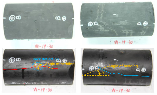

Figure 26.
W–19 triaxial condition hydraulic fracturing pumping curve and acoustic emission positioning.
The W–20 rock sample was drilled at an angle of 60° to the laminae, and there were no obvious cracks or defects on the surface of the rock sample before the experiment. After the experiment, hydraulic fractures were formed on the two symmetrical flanks, and obvious fracture deflection could be observed on the fractures on both flanks. The photograph of the specimen W–20 after the test and the pumping pressure curve are shown in Figure 27. The deflection angle was approximately equal to the angle between the laminae and the borehole axis at the deflection point, and the deflection angle gradually decreased with the expansion of the fractures and, finally, was roughly parallel to the borehole axis.
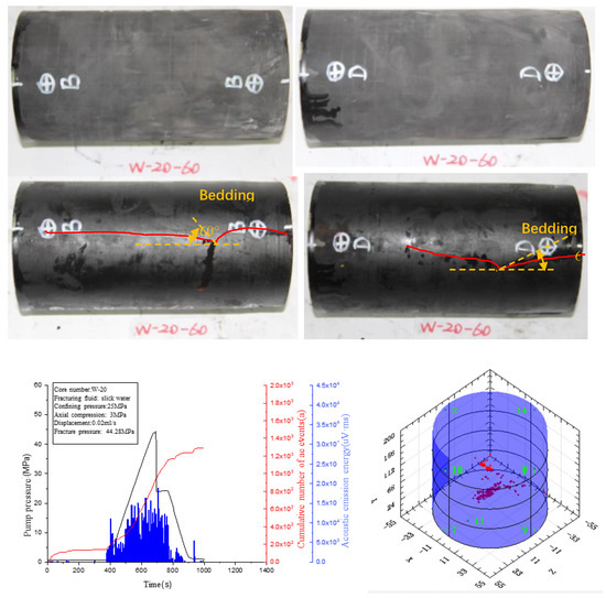
Figure 27.
W–20 triaxial conditional hydraulic fracturing pumping curve and acoustic emission localization.
As shown in Figure 28, the experimental results under 25 MPa peritectic pressure conditions show that the smaller the lamina angle is, the smaller the shale fracture pressure is, and the maximum is at the vertical lamina coring. For the rock samples W–19 and W–20 with lamina angles, both hydraulic fractures deflected approximately parallel to the shale lamina near the middle of the core after fracturing the rock samples; however, for rock samples with vertical lamina coring (90°), such as W–11, a flat hydraulic fracture along the borehole axis was basically formed after hydraulic fracturing, and generally, no deflection occurred. This indicates that in the presence of a laminar dip, the laminar angle of the core has an effect on the formation and extension of the hydraulic seam. Shale laminae have a lower strength than shale bodies, and the laminae joints are easily damaged by tension under hydraulic pressure. The hydraulic joints also tend to expand along the laminae joints, and deflection occurs under conditions with a certain laminae angle because the fracture expansion is not only influenced by the mechanical properties of the rock itself but also influenced by the external loading method. In addition, the strength of shale laminae is weaker than that of shale proper, thus leading to a lower fracture pressure in the presence of laminae angles during fracturing. By comparing the before and after fracturing specimen photos of the rock samples W–19 and W–20, it can be seen that the positive stress acting on the laminar joints increases with an increasing laminar inclination angle, the difficulty of shear damage along the laminar surface increases, it is more difficult to communicate the laminar surface, and the complexity of the joint network decreases. The physical simulation laminar inclination angle is set to the laminar and longitudinal angle, while the numerical simulation laminar inclination angle is set to the laminar and horizontal direction angle. Therefore, the physical model test results are consistent with the numerical simulation experimental results, which verifies the reliability of the numerical simulation results.
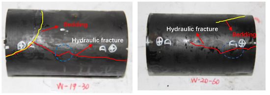
Figure 28.
Experimental results of different laminar surface inclination angles.
4. Conclusions
- The influence of laminae on the expansion pattern of artificial cracks is mainly affected by various factors, such as the original ground stress state, the cementation strength of laminae joints, and the approach angle of artificial cracks. The numerical calculation results show that the hydraulic fracture first expands in the direction perpendicular to the minimum horizontal principal stress after starting from the injection point, and after encountering the laminated joints, the hydraulic fracture turns and expands along the side of the laminated surface.
- The expansion process of hydraulic fracture under different horizontal ground stress conditions is simulated by using the global embedding cohesive unit method, and under the same conditions, a certain horizontal ground stress difference can induce hydraulic fracture to form a more complex seam network. However, with the further increase in the horizontal ground stress difference, the vertical stress difference coefficient increases, the probability of hydraulic fracture penetration along the longitudinal direction of the maximum principal stress increases, the horizontal laminar surface of communication decreases, and the complexity of the fracture network decreases.
- It can be seen from the numerical simulation and physical model experiments that with the increase in the laminar dip angle (angle between the lamina and horizontal direction), the positive stress acting on the laminated joints decreases, the frictional resistance between the laminated surfaces decreases, and shear damage along the laminated surfaces is more likely to occur, so the distance between the communicating laminated joints and the complexity of the joint network increase.
- By simulating the hydraulic fracture expansion process of rocks under different cementation surface strength conditions, it is found that as the cementation strength of laminated surfaces decreases, the tensile strength of laminated surfaces decreases, the hydraulic fracture is more likely to induce shear slip of the laminated surfaces, and the fracture complexity increases significantly.
- In this study, the interaction mechanism and influencing factors between laminae and hydraulic fracture extension were studied from the two perspectives of numerical simulation and physical model testing, but there were biases in the specimen itself because the cylindrical specimens used were outcrops. In future work, we will combine manual sample making and downhole cores to exclude the interference of the specimen itself and conduct a more systematic and comprehensive study.
Author Contributions
Data curation, S.L.; Formal analysis, Z.H.; Methodology, Z.H. and X.C.; Writing—original draft, Z.H.; Writing—review and editing, Z.H. and X.C. All authors have read and agreed to the published version of the manuscript.
Funding
This work was supported by the Open Fund of State Key Laboratory of Shale Oil and Gas Enrichment Mechanisms and Effective Development (Grant No. 35800000-20-ZC0607-0019).
Institutional Review Board Statement
Not applicable.
Informed Consent Statement
Not applicable.
Data Availability Statement
Not applicable.
Conflicts of Interest
The authors declare no conflict of interest.
References
- Zou, C.; Zhai, G.; Zhang, Y.; Wang, H.; Zhang, G.; Li, J.; Wang, Z.; Wen, Z.; Ma, F.; Liang, Y.; et al. Global conventional−unconventional oil and gas formation distribution, resource potential and trend forecast. Oil Explor. Dev. 2015, 42, 13–25. [Google Scholar]
- Jiang, Z.; Zhang, W.; Liang, C.; Wang, Y.; Liu, H.; Chen, X. Basic characteristics of shale oil reservoirs and evaluation elements. J. Pet. 2014, 35, 184–196. [Google Scholar]
- Zhang, J.; Lin, L.; Li, Y. Shale oil classification and evaluation. Geosci. Antecedents 2012, 19, 322–331. [Google Scholar]
- Lu, S.; Xue, H.; Wang, M.; Xiao, D.; Huang, W.; Li, J.; Xie, L.; Tian, S.; Wang, S. Exploring the evaluation criteria of shale oil and gas resources classification. J. Pet. 2016, 37, 1309–1322. [Google Scholar]
- Lu, S.; Xue, H.; Wang, M.; Chen, F.; Huang, W.; Li, J.; Wang, W.; Cai, X. Exploring the evaluation criteria of shale oil and gas resources classification. Oil Explor. Dev. 2012, 39, 249–256. [Google Scholar]
- Zou, C.; Zhu, R.; Bai, B.; Yang, Z.; Hou, L.; Zha, M.; Fu, J.; Shao, Y.; Liu, K.; Cao, H.; et al. Meaning, Characteristics, Potential and Challenges of Tight Oil and Shale Oil. Bull. Miner. Rock Geochem. 2015, 34, 3–17. [Google Scholar]
- Lin, S.; Zou, C.; Yuan, X.; Yang, Z. Current status of tight oil development in the U.S. and insights. Rocky Reserv. 2011, 23, 25–30, 64. [Google Scholar]
- Pramod, K. Woodford growing revenues by farming to oil shale. World Oil 2012, 233, 32. [Google Scholar]
- Zhao, J.; Fang, C.; Zhang, J.; Wang, L.; Zhang, X. Evaluation of Shale Gas Selection Areas in China from North American Shale Gas Exploration and Development. J. Xi’an Univ. Pet. 2011, 26, 1–7. [Google Scholar]
- Guan, W. Study on the evaluation criteria of the “sweet spot” of inter−salt shale oil in Qianjiang Depression. J. Jianghan Pet. Staff. Univ. 2020, 33, 15–17. [Google Scholar]
- Fan, S. Pore Structure Characteristics and Influencing Factors of the Inter−Salt Shale Oil Reservoir in Qianjiang Depression, Qianjiang Section 3; China University of Petroleum: Beijing, China, 2020. [Google Scholar]
- Zhang, C. Oil−Bearing and Movability Analysis of Inter−Salt Shales of Qianjiang Formation in Qianjiang Depression, Jianghan Basin; China University of Petroleum: Beijing, China, 2020. [Google Scholar]
- Xu, E.; Tao, G.; Li, Z.; Wu, S.; Zhang, W.; Rao, D. Microscopic reservoir characteristics of different petrographic phases of inter−salt shale oil reservoirs in Qianjiang Depression, Jianghan Basin—Example of 4 subsections of 10 rhymes in three sections of the Paleoproterozoic Qianjiang Formation. Pet. Exp. Geol. 2020, 42, 193–201. [Google Scholar]
- Hu, G. Analysis of the influence of mechanical parameters of stratified shale on fracture morphology of hydraulic fracturing. Drill. Eng. 2022, 49, 97–103. [Google Scholar]
- Wang, Y.; Han, D.; Zhao, L.; Mitra, A.; Aldin, S. An experimental investigation of the anisotropic dynamic and static properties of eagle ford shales. In Proceedings of the SPE/AAPG/SEG Unconventional Resources Technology Conference, Denver, CO, USA, 20–22 July 2019; p. 304. [Google Scholar]
- Du, M.; Pan, P.; Ji, W.; Zhang, Z.; Gao, Y. Spatial and temporal characteristics of the damage process in carbonaceous shale Brazil under cleavage load. Geotechnics 2016, 37, 3437–3446. [Google Scholar]
- Ma, X.; Li, C.; Bai, J.; Ma, Z. Analysis of physical characteristics of shale rock based on ultrasonic testing. Oil Geophys. Prospect. 2021, 56, 801–808. [Google Scholar]
- Chen, X.; Liu, R.; Xie, B.; Pan, Y.; He, X. Capacity model for fractured horizontal wells in shale reservoirs considering laminar seams. Xinjiang Oil Gas 2022, 18, 73–79. [Google Scholar]
- Heng, S.; Yang, C.; Guo, Y.; Wang, C.; Wang, L. Study on the influence of laminae on shale hydraulic fracture extension. J. Rock Mech. Eng. 2015, 34, 228–237. [Google Scholar]
- Liu, Z.; Feng, Q.; Wang, Y.; Wang, H.; Zou, L.; Tang, J. Fracture height prediction model and construction optimization method for fracturing Weiyuan shale gas reservoirs considering the influence of stratigraphy. Logging Technol. 2022, 1, 114–121. [Google Scholar]


Publisher’s Note: MDPI stays neutral with regard to jurisdictional claims in published maps and institutional affiliations. |
© 2022 by the authors. Licensee MDPI, Basel, Switzerland. This article is an open access article distributed under the terms and conditions of the Creative Commons Attribution (CC BY) license (https://creativecommons.org/licenses/by/4.0/).