1. Introduction
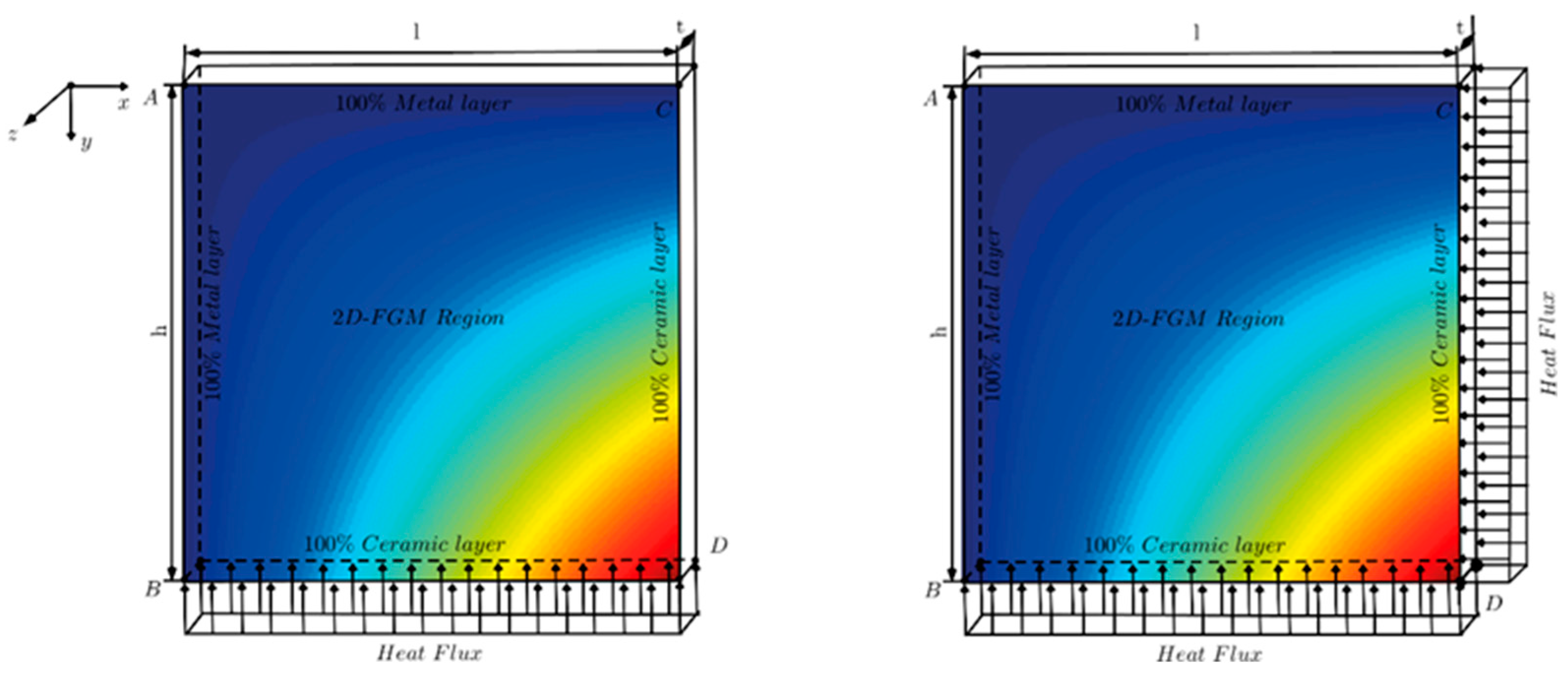
As space technologies have evolved, the use of conventional composites has been limited. Therefore, FGM is suggested as an effective material idea for ultimate thermal and mechanical loads. FGM is metal on one side and ceramic on the other, and the composition changes depending on the volume fraction. Thus, the thermal resistance of the ceramic and the strength of the metal are utilized at the maximum level.
In the last two decades, many studies have been conducted on the determination of the mechanical behavior of FGMs [
1,
2,
3,
4,
5,
6,
7,
8]. However, due to the difficulties encountered in production, the use of FGMs in the industry has been limited [
9,
10]. Therefore, many studies have focused on finding the optimum compositional gradient exponents that determine the volumetric distribution theoretically [
11,
12,
13,
14,
15,
16].
However, although mass production has not yet been made for FGM, polymer and metal-based FG materials have started to be produced with the spread of additive manufacturing methods and these studies have begun to take place in the technical literature [
17,
18,
19,
20].
Moita et al. [
21] used a gradient-based optimization algorithm for material distribution and sizing in free vibration and linear buckling problems of FGMs. Mantari and Monge [
22] used a new optimized hyperbolic displacement in combination with Carrera’s Compound formulation for free vibration and buckling problems of FGM sandwich plates. Ashjari and Khoshravan [
23] investigated mass optimization of FGM for stress analysis of the bending fraction. They applied genetic algorithms and herd optimization to the models they designed. As a result, they emphasized that particle swarm optimization outperforms the genetic algorithm when we look at the convergence rate and accuracy. Nazari et al. [
24] tried to estimate the core thickness and volume ratio and the three-dimensional natural frequency of the FGM sandwich rectangular plate with the Meshless Local Petrov-Galerkin Method and Artificial Neural Networks (ANNs). Roque and Martins [
25] used the Differential Evolution (DE) algorithm as a guide to finding the optimum design in the free vibration analysis of FG nanobeams. Correia et al. [
26] optimized the minimum mass and minimum material cost for the FGM plates. The Simulated Annealing (SA) method is used to find the optimal design of the FGM. They emphasized that this model is easily applicable for different metal and ceramic materials within the p-index and production constraints. Maciejewski and Mroz [
27] investigated the optimal composition of complex shaped FGM for thermomechanical behavior. Nguyen and Lee [
28] modeled a thin-walled FG beam under buckling for beam section and material optimization.
Innovative materials, which are used in sensitive machine elements and materials under critical operating conditions and whose structure can change according to the problem, are gaining more and more importance day by day. For this reason, optimization approaches that reach the right result in effective time have been developed for different problems at certain limit values. Studies aimed to find the optimum material composition or lead the optimization in different methods such as artificial neural network, hybrid algorithms, multi-object, iso-geometric, topology optimization [
29,
30,
31,
32,
33,
34,
35,
36,
37]. Genetic programming provides a formula by facilitating the solution path in numerical or non-numerical problems, so that the solutions to be obtained as a result of long efforts are simplified. The performance of genetic programming is tested and applied to capacity estimation, hydrology, multidimensional problems. Since it is a new method, there are very few studies in the field of FGM [
38,
39,
40,
41,
42,
43,
44]. When the genetic programming applied in composite materials is examined; There are studies such as coating quality, strength, and frequency of the material. Some of these studies are exemplified below.
Gu et al. [
45] used deep learning and genetic programming to predict the bond strength capacity in adhesive joints used in composite plates. They emphasized that in both developed models, optimum structure and material design are estimated efficiently. According to Dehestani et al. [
46] estimated the microhardness of the Ni/Al
2O
3 nanocomposite coating with the model created by combining genetic programming and genetic algorithm methods in gene expression programming (GEP).
Shakeri [
47] created a mathematical model with genetic programming and investigated the relationship between the coating quality of the composite material and the coated weight. With this model, the relationship between the coating material and coating time, and coating quality is determined. According to Punugupati et al. [
48] investigated the effect of porosity on the flexural strength of composite material under load. Using MGGP, they created an efficient model between flexural strength and ceramic porosity, and solid loading. According to Sharif et al. [
49] proposed a genetic programming model to reduce the magnetic resonance of composite materials. They noted that the model in GP outperformed the methods previously suggested in the literature. According to Demirbas et al. [
50] found the relationship between the thermo-mechanical behavior of GP and 1-D FG rectangular plates and the material composition by constructing a model. They showed that the formulas and equations reached by GP converged to the real values at a high rate and the numerical analysis time became efficient.
In this study, an efficient working model was created by obtaining data sets with compositional gradient exponent values in both directions using MGGP and equivalent stress levels found by the finite difference method (FDM) of the 2D-FG plate. In these models, the input data is the compositional gradient exponent and the output data are equivalent stress levels, and formulas that give the relationship between input and output with MGGP models are obtained, thus reducing CPU processing time.
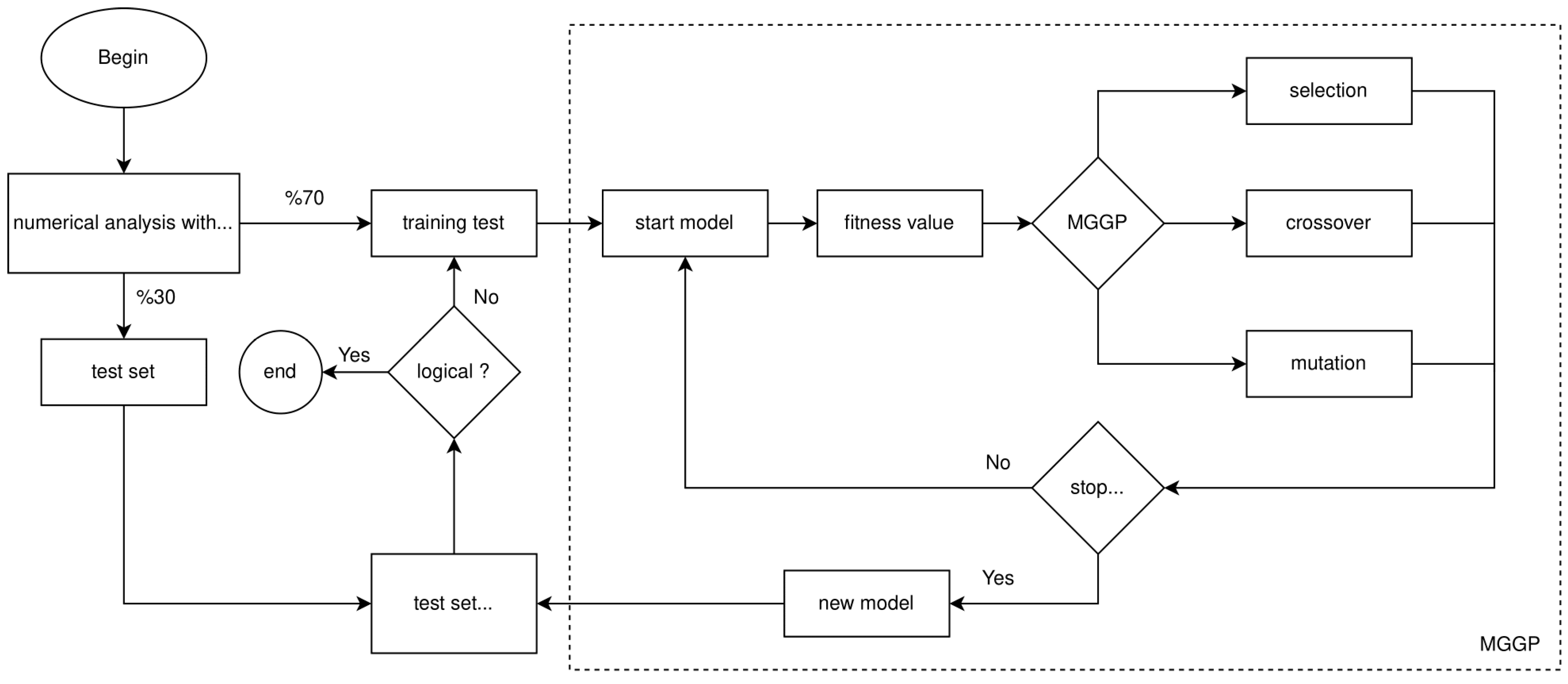
3. Application in GP Programming
Performance of MGGP can be determined by fitness, maximum error, minimum error, and standard deviation. These are created after training value and test value.
Table 3 shows the simulation results of Model 1 and Model 2. In Model 1, best fitness value
, maximum error value
, minimum error value
and standard deviation
are found in training results. In Model 2, best fitness value
, maximum error value
, minimum error value
and standard deviation
are found in training results. In Model 1, best fitness value
, maximum error value
, minimum error value
and standard deviation
are found in test results. In Model 2, best fitness value
, maximum error value
, minimum error value
and standard deviation
are found in test results. When we look at these values, we see that best produced equivalent stress value is
for Model 1 and
for Model 2.
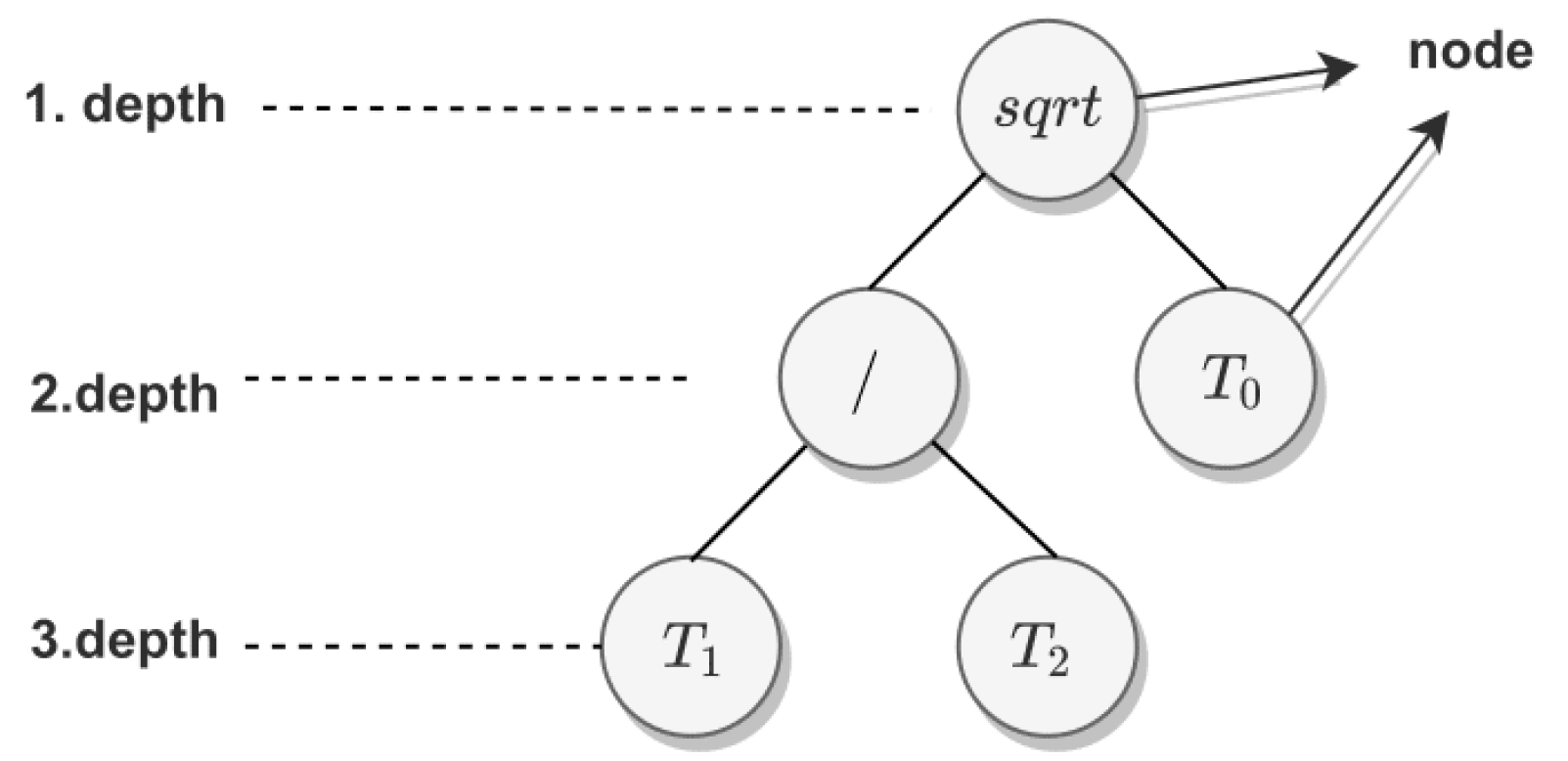
Table 4 contains information on tree structures of the best models of Model 1 and Model 2. When all stress values are examined, gene and tree depths are reached at maximum values. When tree depth investigated by complex structure and node number, least node and minimum complex structure are seen in
for Model 1 and in
for Model 2. When all the models are studied, the most complex structure and maximum number of nodes occurred in
of Model 2.
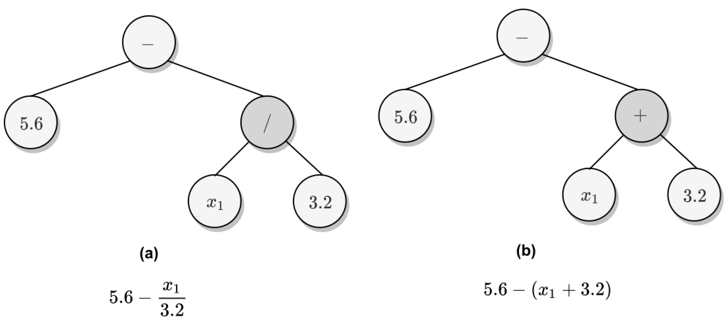
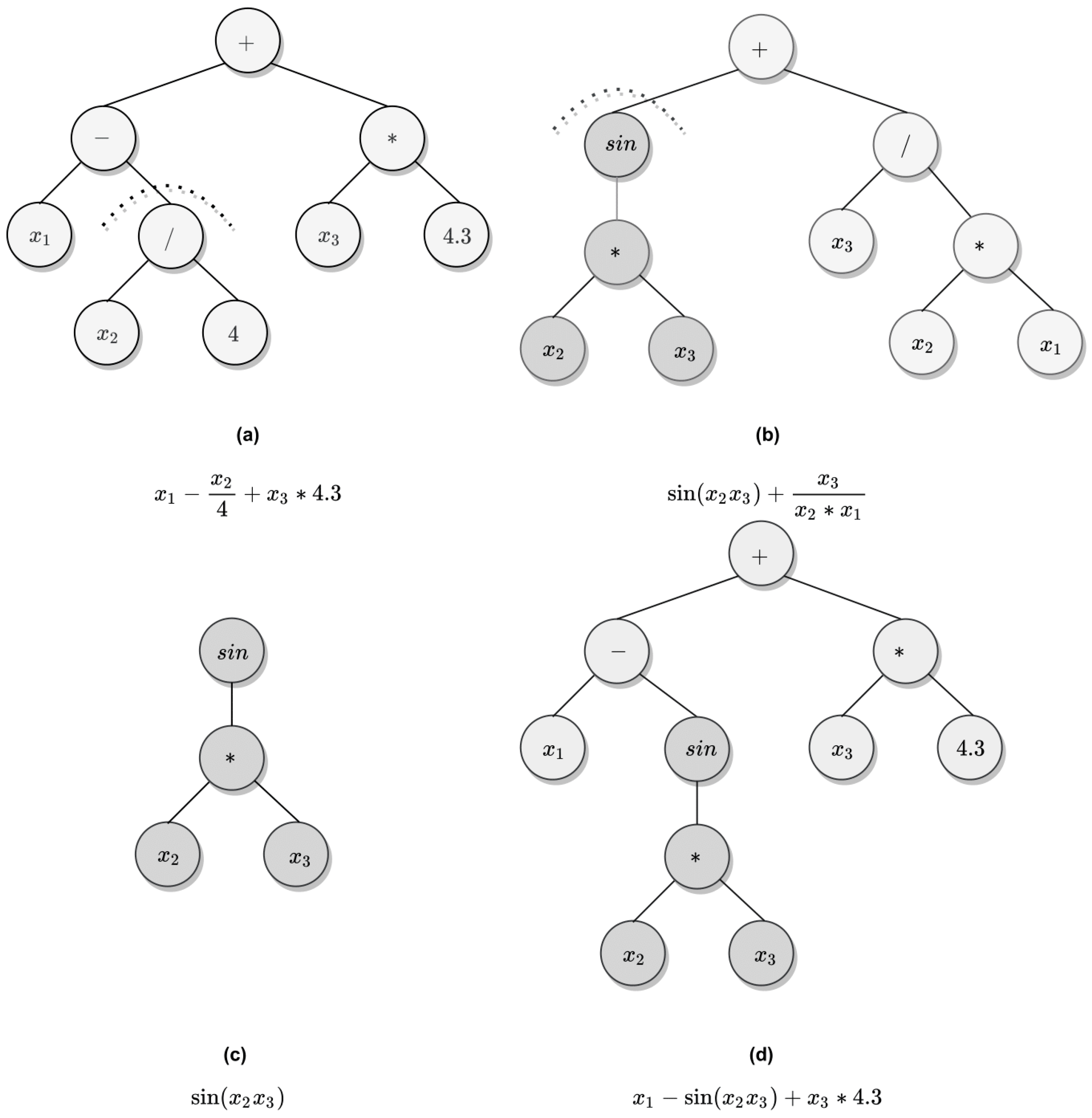
In our study, the best equations of MGGP are shown in
Table 5. As we have explained in the other tables, the most complex equations are seen in
in Model 2. All equations can be used as a guide in optimization for researchers.
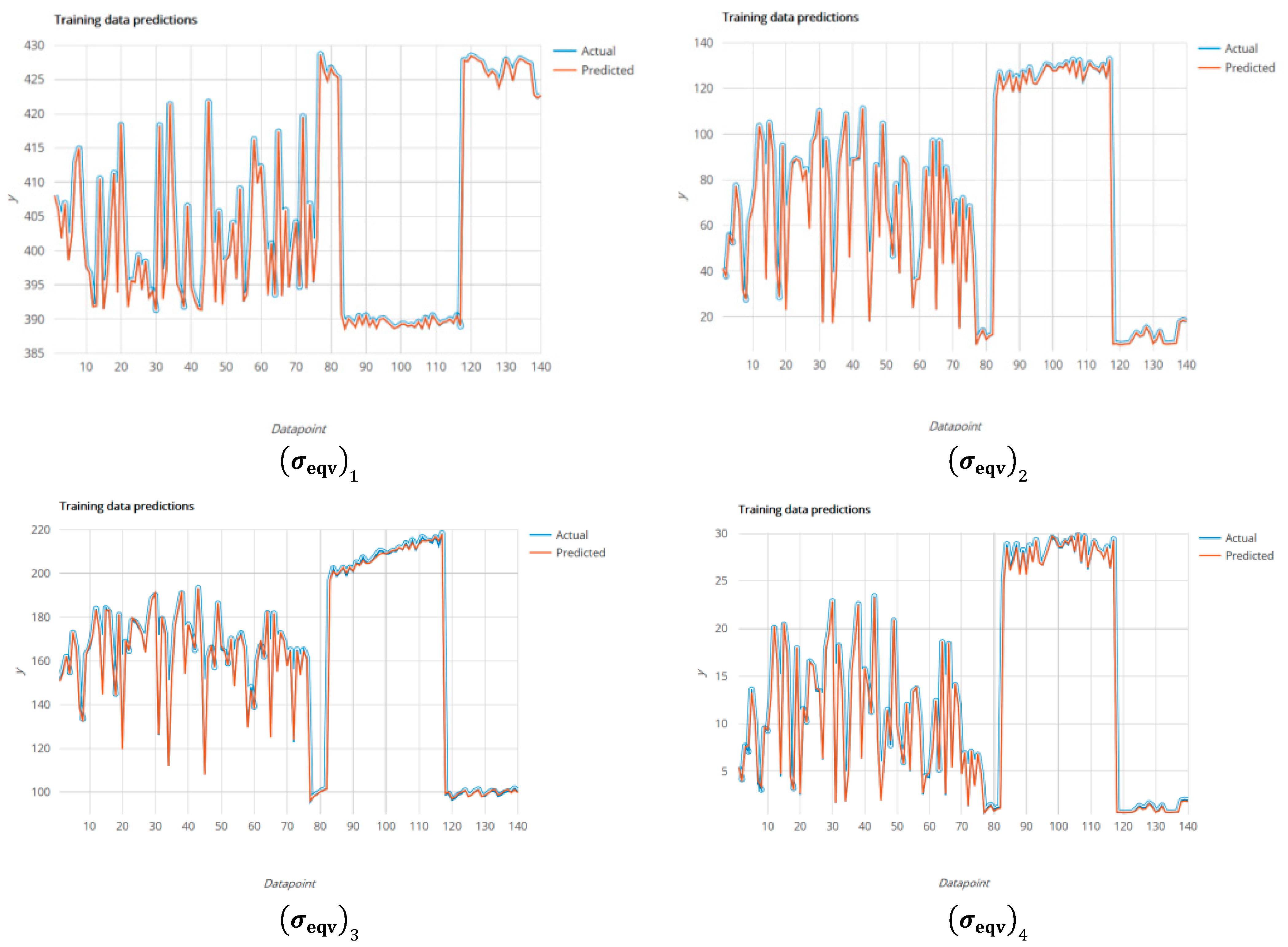
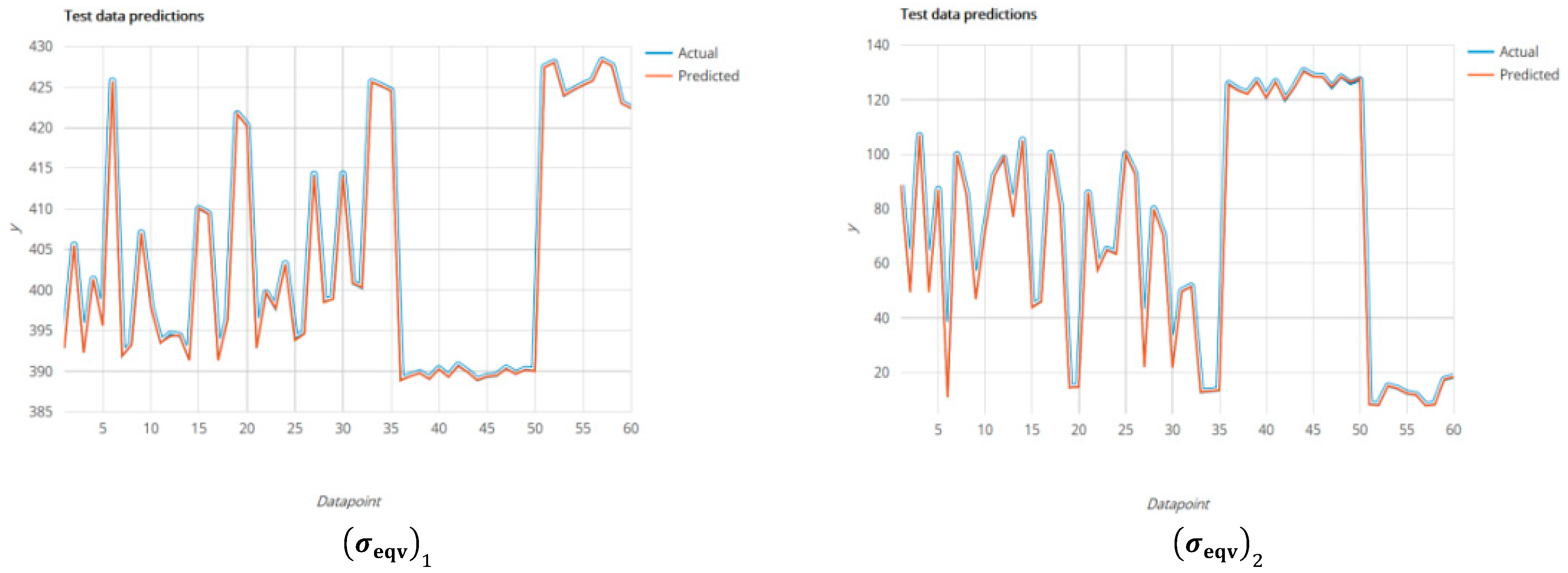
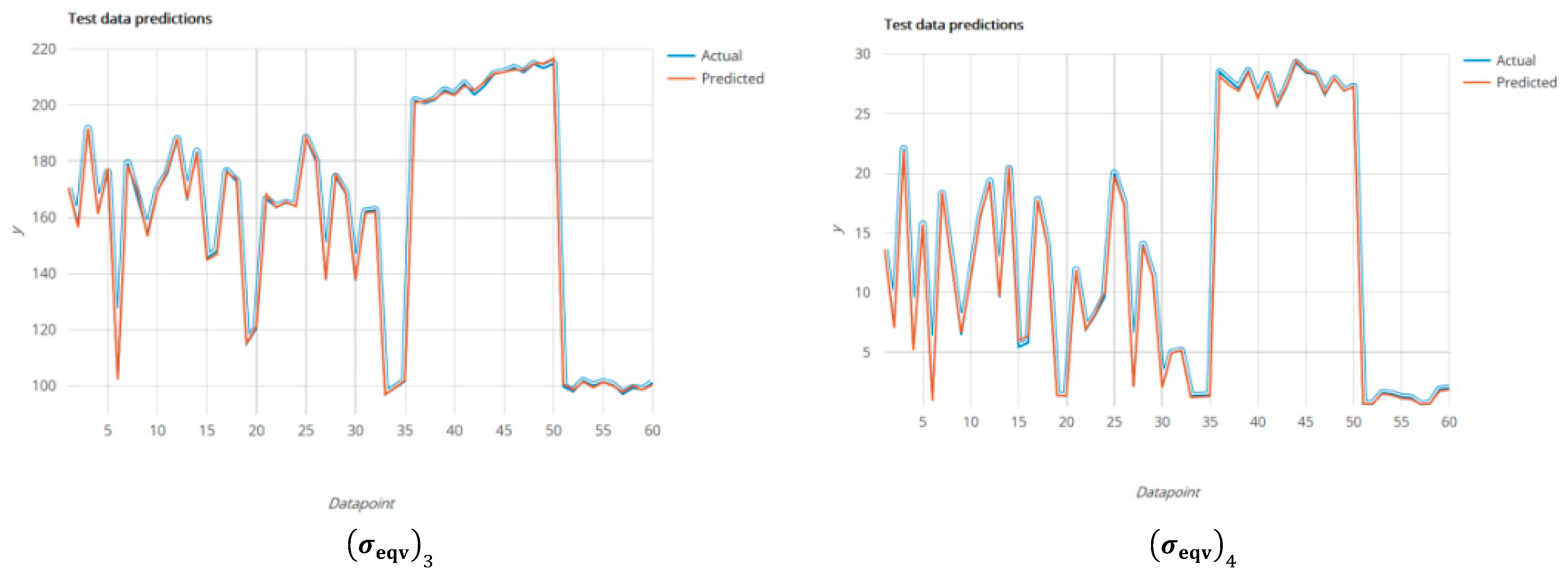
The results obtained from the numerical analysis results are compared with the values obtained in genetic programming. Considering the order of the input data, graphs are created with the equivalent stress value, which is our output data. It is important that the figures in the graphics are similar to each other in order to check whether the program is working correctly. When we look at all the graphics, it is remarkable that they are similar to each other.
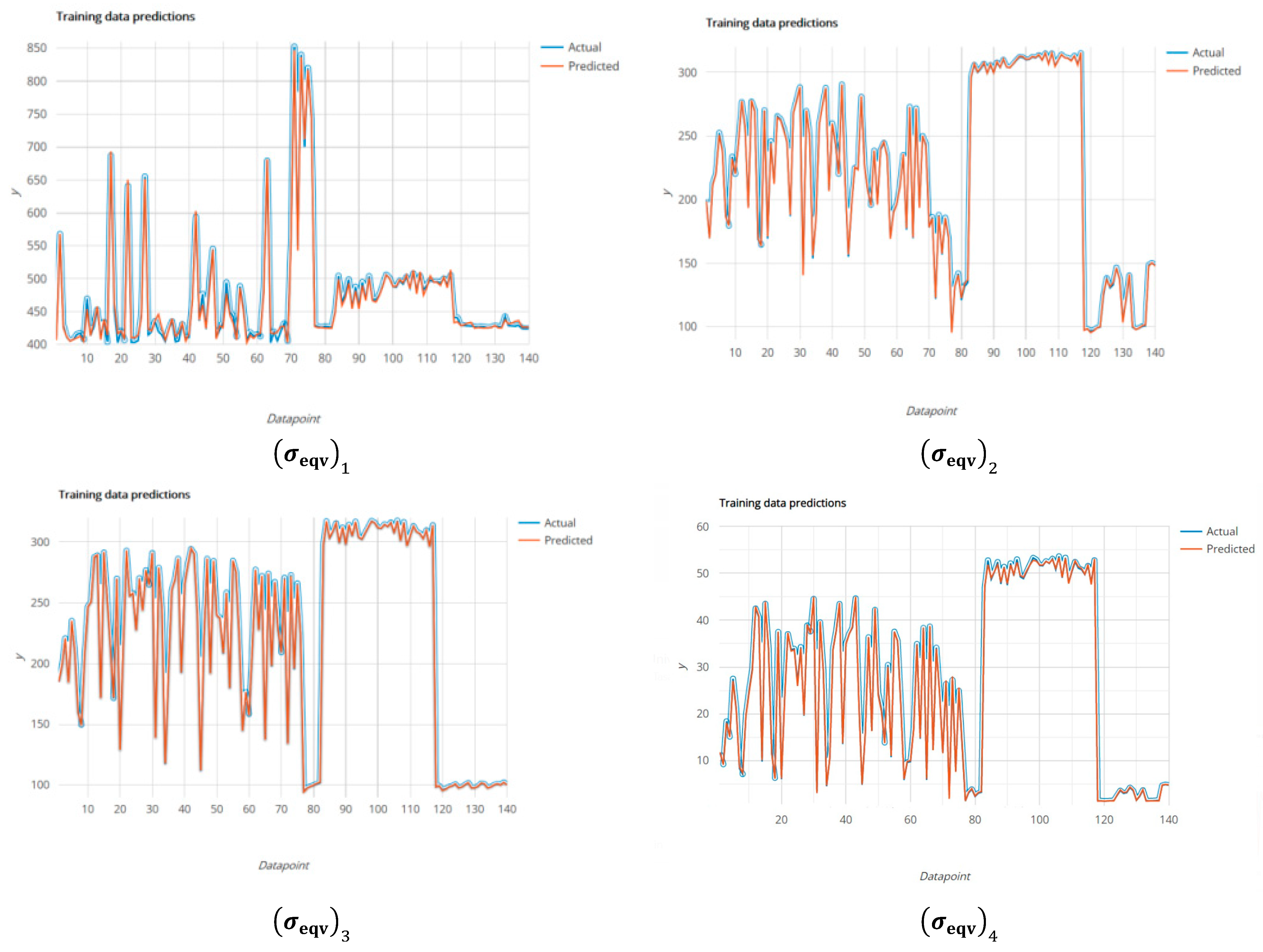
Figure 6 shows the graph of the actual and predicted values of the training simulation results of all equivalent stresses of Model 1, and
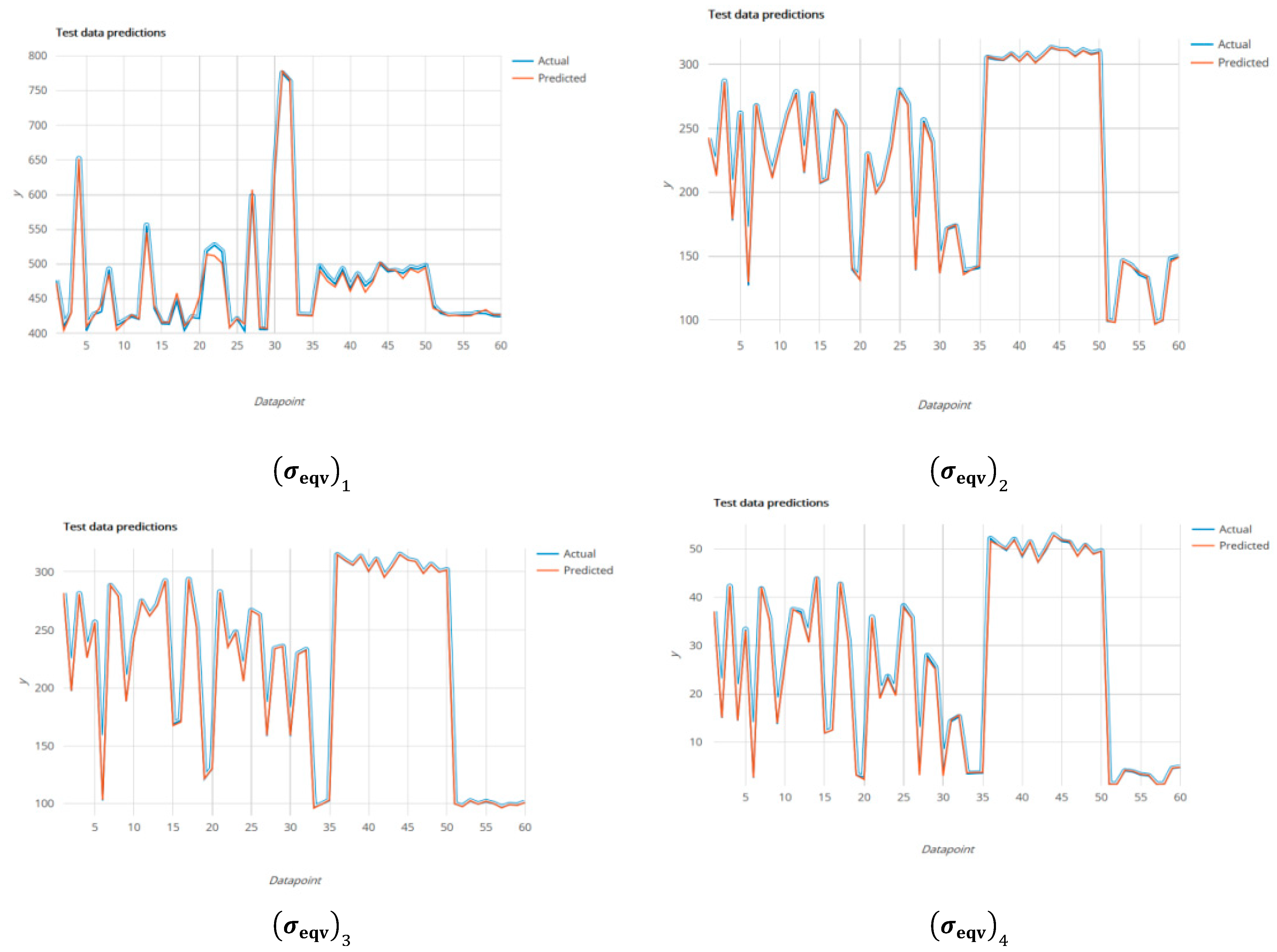
Figure 7 has test simulation results. In error graphs, it is desired that the actual value and the predicted value be very close to each other. For both training and test simulation results, the actual and predicted values in the graphs converged.
Figure 8 shows a graph of the actual and predicted values of the training simulation results of all equivalent stresses of Model 2, and also
Figure 9 shows test simulation results of Model 2. Graphics show that MGGP solved all equivalent stresses with high accuracy.
The performance of 200 different compositional gradient exponent values evaluated with equations produced in MGGP. Results of found equations reached the effective solution with high accuracy. The RMSE, error rate, minimum and maximum error values of Model 1 obtained by looking at the actual and predicted values of all equivalent stresses are shown in
Table 6. Considering these criteria, in terms of efficiency,
values reached the best solution and
values reached the worst solution.
The RMSE, error rate, minimum and maximum error values of the Model 2 achieved from actual and predicted values of all equivalent stresses are shown in
Table 7. When Model 2 examined by these criteria,
values reached the best solution and
values reached the worst solution.
To determine the average duration of the numerical solution, an average time estimate is made by choosing the largest, medium, and smallest values of values between 0.0001–1.5. These time expressions are shown in
Table 8. Based on these times, the average times are 2049.47 s in Model 1 and 842.00 s in Model 2. Regardless of the data set formation time of MGGP, one n-m compositional gradient exponent value is reached in less than one second after the model is created, and thus CPU time is reduced and work time saved.


