Robust Feature Selection-Based Speech Emotion Classification Using Deep Transfer Learning

Abstract

Speech Emotion Classification (SEC) relies heavily on the quality of feature extraction and selection from the speech signal. Improvement on this to enhance the classification of emotion had attracted significant attention from researchers. Many primitives and algorithmic solutions for efficient SEC with minimum cost have been proposed; however, the accuracy and performance of these methods have not yet attained a satisfactory point. In this work, we proposed a novel deep transfer learning approach with distinctive emotional rich feature selection techniques for speech emotion classification. We adopt mel-spectrogram extracted from speech signal as the input to our deep convolutional neural network for efficient feature extraction. We froze 19 layers of our pretrained convolutional neural network from re-training to increase efficiency and minimize computational cost. One flattened layer and two dense layers were used. A ReLu activation function was used at the last layer of our feature extraction segment. To prevent misclassification and reduce feature dimensionality, we employed the Neighborhood Component Analysis (NCA) feature selection algorithm for picking out the most relevant features before the actual classification of emotion. Support Vector Machine (SVM) and Multi-Layer Perceptron (MLP) classifiers were utilized at the topmost layer of our model. Two popular datasets for speech emotion classification tasks were used, which are: Berling Emotional Speech Database (EMO-DB), and Toronto English Speech Set (TESS), and a combination of EMO-DB with TESS was used in our experiment. We obtained a state-of-the-art result with an accuracy rate of 94.3%, 100% specificity on EMO-DB, and 97.2%, 99.80% on TESS datasets, respectively. The performance of our proposed method outperformed some recent work in SEC after assessment on the three datasets.

1. Introduction

SEC occupies an important position in affective computing and plays a cogent role in human relationships. Psychologically, there is no better way: a relationship can neither be initiated nor sustained without adequate communication. However, communication takes place in many ways (verbal and non-verbal), but auditory speech communication has been the hub for all other forms. It is the nucleus to which all other means of human interaction revolve [1]. One major factor that determines human decisions is emotion [2,3]. Whether on an inter-personal or intra-personal basis, emotion influences why human beings act or react the way they act, informs their judgment, and even sometimes molds their opinions. Classification of emotion through human speech, therefore, is the act of recognizing emotional content from speech [4] as depicted in Figure 1. The growth of human–computer interaction in the last decade cannot be unconnected to SEC [5,6]. Apart from wider application in major fields and sub-fields, SEC is reshaping the nearby future next revolution of human–machine interaction as it is attracting the vast majority of researchers worldwide. Mental disorders and depression-related diseases have been drawing great benefit from SEC coupled with the acceleration of patient treatment [7].

Figure 1. Emotion Classification Framework.

However, the curiosity of why speech emotion classification has been experiencing high processing cost and increased memory consumption with less accuracy has remained a great question among researchers today [8]. Presently, one lingering challenge identified so far is the lack of a sufficient annotated speech dataset, but then, several models have been proposed to mitigate this challenge and improve accuracy, as was obtainable in [9] using Surrey Audio-Visual Expressed Emotion (SAVEE), Ryerson Multimedia Laboratory (RML), and eNTERFACE’05 as the speech corpus. A 3D convolutional neural network (CNN) model with fully connected layers was developed for SEC. They attained a state-of-the-art performance, but the huge features [10] extracted without a corresponding feature selection method applied before actual classification tends to increase computational [11] complexity and reduce the accuracy rate.

By way of improving on the previous study, we proposed a novel and robust deep transfer learning approach for speech emotion classification with feature selection techniques. Transfer learning leverages on knowledge acquired from the source task and implements it on the target task [12]. It reduces computational complexity as it requires no training before its usage. Not all features from speech signals carry emotional content, and this is the reason why many models’ failed to attain an optimal result. There is a need for a mechanism to subject extracted speech features [13,14] (spatial) to selection techniques for effectively identifying discriminating features that can increase accuracy while reducing computational cost.

Main Contributions

The specific contributions of this work are:

• Applying an optimized deep transfer learning for feature extraction using the pretrained model on ImageNet.
• Adopting an efficient feature selection technique for selecting a discriminative feature for optimal classification of emotion, because not all features from a speech signal carry paralinguistic information relevant to accurate emotion classification.
• Reducing misclassification of emotion and computational cost, while achieving state-of-the-art and improving accuracy on three speech datasets with two different classifiers.
• Systematic performance evaluation and critical comparison of the model with other methods, which indicates a high efficiency of deep transfer learning with feature selection for SEC.

The remaining part of this work is arranged as follows. Related work with some useful background concepts is presented in Section 2. Section 3 deals with the proposed methodology of the work. In Section 4, the experimental flow with exact results achieved was presented. Section 5 presents the discussion of the obtained results and comparison with recent works that have been published. A conclusion with recommendation for future work is given in Section 6.

2. Literature Review and Related Works

From a psychological point of view, Refs. [15,16], human emotions are categorized into six major groups, which fall under positive and negative emotion, respectively. However, this can also be sub-divided into valence or arousal. Valence emotion determines the extent to which emotion is either positive or negative, while arousal indicates the level of intensity. The description of these basic enotions are shown in Table 1. These emotions goes through the process of vectorization in speech data processing (encoding) before emotional features extraction and classification can be performed.

Table 1. Basic Emotion Description.

Emotion	Description	Expression	Class
Happiness	A state of pleasantness characterized by joyful mood	Upbeat	Positive
Sadness	A transitional emotion state usually characterized by grieving felling	Leathery and dampened	Negative
Fear	Plays a vital role in survival	Rapid heratbeat	Positive/Negative
Disgust	Results from unpleasant taste or smell	Retching/nauseating	Negative
Anger	A state of hot temper, hostility and aggression	Yelling	Negative
Surprise	Usually occurs when the unexpected happens	Screaming and hilarious	Positive/negative

For more than half a decade, several deep transfer learning techniques rooted in deep convolutional neural network (DCNN) have been applied in speech recognition with the utmost focus on emotion classification from speech. Transfer learning minimized computational cost while maintaining an accurate extraction of features from speech signals [17,18]. Despite several outstanding records of successful application of convolutional neural network (CNN), the SEC domain is still facing the intense challenge of optimal performance with minimal complexity. As the literature is saturated with many of the applications of deep transfer learning techniques for an improved performance in speech emotion classification, this work has reviewed some published works.

Obviously, the recent advancement in Artificial Intelligence and affective computing has conspicuously made the deep transfer learning model very popular in major fields, such as image segmentation, visual objects recognition systems, facial emotion recognition systems, age and gender estimation, and speech recognition systems, which is due to its extraordinary performance in prediction and low error rate.

Vryzas et al. [19] applied a pretrained DCNN-based transfer learning for speech emotion classification. A multi-user speech dataset was used in training their model, while fine tuning took place on the speaker-dependent speech emotion dataset. The first 11 layers of the model that served in feature learning were frozen from being trained according to the structural setup of the model with utmost the aim of fine-tuning the model on the target’s dataset input. Mustaqeem and Kwon, Ref. [20] investigated the possibility of adopting a double stream approach of CNN and DCNN for extracting spectral and spatial features for an improved performance in SEC. Aside from the fusion of dual features techniques, considerable effort was made by applying a feature selection algorithm for the effective classification of emotion. Mustaqeem and Kwon Ref. [21] proposed an attention-based convolutional neural network with a fully connected layer trained in an end-to-end manner for the effective classification of speech emotion. An optimized DNN was proposed by Aouani and Ayed, Ref. [22] for real-time speech emotion classification. The optimization was carried out using stochastic gradient descent.

Learning the most salient features from a speech spectrogram image through a light-weight CNN model for an improved performance in SEC was presented by Anvarjon et al. [23]. The model was also trained in an end-to-end mode, with an enhanced pooling strategy and fewer parameters. A deep transfer learning model that is based on AlexNet with correlation-based feature selection techniques was presented by Farooq et al. [24] in order to investigate the overall impact of the feature selection algorithm on speech emotion classification. Haider et al. [25] evaluated three different feature selection techniques, namely, Relief feature Infinite Latent Feature Selection, and a generalized Fisher score for speech emotion recognition, along with the recently proposed automatic feature selection method. They employed three datasets from three different languages to affirm that higher accuracy can only be achieved through a reduced feature set.

Zhang et al. [26] adopted transfer learning using a pretrained model on ImageNet (AlexNet) to extract segment-level features and an attention mechanism for learning emotionally rich features. Their model also combine Bi-directional Long Short-Term Memory (BiLSTM) for effective speech emotion classification using two different datasets (EMO-DB and IEMOCAP). Feng and Chaspari Ref. [27] proposed a transfer learning technique with distance loss for speech emotion classification. They fine-tuned a siamese nueral network in order to achieve a state-of-the-art result. An experiment was carried out on the eNTERFACE, RAVDESS, and CREMA-D datasets, respectively. Spectrogram features generated from speech signals were augmented in Padi et al. [28] and fed as input into a transfer learning model (ResNet) with a significant pooling layer (statistics) for speech emotion classification. They prevented overfitting and improved classification accuracy in spectrogram augmentation techniques.

Joshi et al. [29] proposed a deep neural network BiLSTM for emotion classification using a cross dataset that was rooted in EEG (electroencephalography). Out of the three datasets (DEAP, SEED, IDEA) used in their work, two were for training, while one (IDEA) was for testing the performance of their proposed method. Four classifiers (SVM, KNN, MLP and Deep RNN) were trained with four speech features (Hjorth parameters, DE, LF-DE and PSD), and the results of their experiments indicated that DNN parameters optimization can positively enhance the performance of the emotion classification system. In addition, the deep BiLSTM model improved emotion recognition from EGG through the extraction of discriminative features and temporal dependencies of speech samples. However, the datasets utilized were insufficient for a typical Deep BiLSTM network model learning, which eventually hampered the accuracy (59%) recorded. The most popular datasets used within the speech emotion domain consist of synthetic data because of the difficulty and security issues associated with real-world speech-based datasets. However, Blumentals and Salimbajevs [30] carried out a speech emotion classification task using a real-world dataset (from phone calls). In their work, a deep learning network made up of two LSTM layers and fully connected layers with an Adam optimizer for back propagation was utilized. Their model was first tested on three popular datasets which included IEMOCAP, RAVDESS and TESS with accuracy of 60.4% and 86.02% before the real-world data obtained from a call center was used. The real dataset was based on Lavitian Language, and a model accuracy of 52.48% was recorded. It very evident from this work that the result is lower than state-of-the-art; moreover, the testing accuracy on the real-world dataset used was not stated.

Really, it is very cumbersome to build a standardized speech corpus for emotion recognition, and this is a major difficulty confronting speech-based emotion classification tasks. Some of these deep learning methods adopted so far require extensive training, which in most cases increases computational cost. However, the accuracy of speech emotion classification must need to be improved upon, as proposed in our study. Additionally, determining which set of features carries emotional information through the feature selection algorithm can lessen misclassification and increase model performance. In Table 2, a summary of the reviewed literature is given.

Table 2. Summary of Related Works.

Author	Techniques	Dataset	Accuracy/ Unweighted Average Recall (UAR)	Number Emotion
Joshi et al. [29]	DNN-BiLSTM	EEG	58.44%	-
Blumetals and Salimbajos [30]	DNN-LSTM	TESS, RAVDESS, IEMOCAP	86.02%	7, 4
Padi et al. [28]	ResNet	IEMOCAP	66.02%	4
Feng and Chaspari [27]	SiameseNet	RAVDESS	32.8% (UAR)	7
Zhang et al. [26]	DCNN-BiLSTMwA	EMODB, IEMOCAP	87.86%, 68.5%	7, 4
Haider et al. [25]	AFS-SVM	EMODB, EMOVO, SAVEE	76.9%, 41.0%, 42.4% (UAR)	6
Farooq et al. [24]	DCNN-CFS	EMODB, SAVEE, IEMOCAP, RAVDESS	95.10%, 82.10%, 83.30%, 81.30%	7, 4
Anvarjon et al. [23]	CNN	IEMOCAP, EMODB	77.01%, 92.02%	7, 4
Aouani and Ayed [22]	DNN	EMODB	96.97%	7
Mustaqeem and Kwon [21]	DNN-INCA	EMODB, SAVEE, RAVDESS	95.0%, 82.0%, 85.0%	7
Vryzas et al. [19]	CNN-VGGNet	Personalized(Web Crowd Sourcing)	69.9%	-

3. Methods and Techniques

A unique approach of DNN-NCA-MLP (Deep transfer learning with Neighborhood Component Analysis and Multi-Layer Perceptron) for speech emotion classification is introduced. At first, our proposed method carried out preprocessing on a raw speech signal to generate suitable input (Mel-spectrogram) for the model. The structural framework of the proposed model is shown in Figure 2 below. The input image generated from the audio signal is fed into the pretrained DCNN model for robust utterance-level [31] features extraction. Thereafter, a feature selection technique is applied to carefully determine relevant and pertinent features for the accurate classification of emotion with the chosen classifier at the top layer of the model.

Figure 2. Structure of the Proposed Model.

3.1. Speech Data Pre-Processing

Any successful SEC model begins with speech database preparation. Most speech emotion corpus are influenced by speakers’ age, gender and cultural background, among others. It then becomes necessary to diligently carry out adequate preparation of the dataset. Unlike other image processing sub-fields, applying transfer learning to a speech-based task requires substantive data preprocessing in order to make the input image suitable for the deep learning network. Specifically, speech signals carry information such as the sampling ratio, frequency and speed that must be enhanced before their usage for training and the corresponding feature map.

The required input to our proposed model is log mel-spectrogram. This is extracted from the speech signal. Mel-spectrogram has proven to be efficient and rich in emotional content for speech emotion classification. In generating the mel-spectrogram, a series of operations such as pre-emphasis, framing and windowing must need to be performed. The speech signal is first subjected to pre-emphasis for amplification of the frequency. Because of the continuous nature of the speech signal, framing is performed to disintegrate the signal into a fixed-length size, after which a hamming window of 20 ms size function is applied on the frame with 10 ms shift, as computed in Equation (1)

$$w\left(n\right)=0.54-0.46cos\left(\frac{2\pi n}{M-1}\right)0\le n\le M-1$$

(1)

where M represents the window size for the hamming function w(n).

The mel-filter bank used in this work is 40, while the sample rate is 16 kHz and FFT (Fast Fourier Transform) is 512. A speech signal (x) of length (N) can be converted into a signal in the frequency domain (X) using the FFT technique as computed in Equation (2). The size of FFT corresponds to the size of the last convolution layer of our pretrained model. FFT is adopted [32] in generating the complete mel-spectrogram of the speech sample. As part of preprocessing, the mel-spectrogram generated using FFT is resized to the input specification (size) of our proposed model, which is 224 × 224 × 3. This represents the size (height × width) and the number of channels, respectively.

$$X\left(t\right)={\mathsf{\Sigma }}_{r=1}^{N-1}\left(x\left[r\right]Wcos\frac{n\pi x}{L}+b_{n}sin\frac{n\pi x}{L}\right)$$

(2)

where x(r) represents a signal, W represents an N-point window function and h = 0, 1, 2, …, N− 1.

3.2. Feature Extraction with Deep Convolutional Neural Network

This section gives the detail performance of our proposed model with respect to feature learning from the original input mel-spectrogram. An utterance level feature is extracted using VGGNet (Visual Graphics Group Network) as the base model for the deep transfer learning model. As shown in Figure 2, the model consists of five, 2D convolutional layers in series of 224 × 224 × 3, 112 × 112 × 128, 56 × 56 × 256, 28 × 28 × 512 and 14 × 14 × 512 kernel size. Altogether, four pooling layers were used, with the last pooling layer having a size of 7 × 7 × 512. A dropout layer and two dense layers with ReLu (Reactivation Linear Unit) were used as the topmost level of the feature extraction segment. The dropout layer is a hyperparameter that can be used to prevent overfitting [33], and ReLu is the activation function. The pretrained model also carries an internal linear activation unit. The model is properly fine-tuned in order to extract all features (global and spatial) before the selection of high-level features in the next section. We utilized sparse-categorical cross-entropy and an Adams optimization algorithm in compiling our model.

The number of trainable parameters for our model is obtained from the fully connected layers (dense layer), because our base model does not need training. The dense layer consists of a total number of neurons from the current layer ($nc$) and previous layer ($np$). The product of these two mini parameters plus one (bias term) gives the value for the dense layer, which represents the total number of trainable parameters for our model. For instance, the single dense layer of our model (Desnse-1), $nc=7,np=512$; therefore, total parameters = $7\times (512+1)=3591$.

3.3. Neighborhood Component Analysis (NCA) Feature Selection

After the extraction of features with the DCNN segment of our proposed model, it is necessary to select relevant features in order to prevent misclassification and increase the accuracy of the entire model. Feature selection [34] occupies a significant position in this work, as it determines the level of performance. Many models other than the proposed model could have yielded an optimal result in speech emotion classification, but the absence of an appropriate feature selection algorithm incapacitated those models. It is very essential to know that huge features from speech data can be extracted, but not all these features are relevant [35] for emotion classification. The more irrelevant the features in the classifier, the greater the likelihood of misclassification and reduction in the accuracy and efficiency of the SEC model. However, even though feature selection is important, a careful choice of which feature selection techniques perform best and under which condition is another dicey question. The choice must be made depending on the model architectural framework. In this work, NCA, a feature selection method based on distance, has been chosen for selecting discriminative features and its performance in maximizing classification accuracy. The normalized equation for computing the NCA feature selection for a multi-class SEC problem is given in Equation (3).

$$S=\{(x_i,y_i),i=1,2,\dots ,n\}$$

(3)

where n is the number of observations, $x_i\in {\mathbb{R}}^p$ denotes the feature vectors, $y_i\in$ {1, 2, …, c} denotes class labels of emotional features, and c is the number of emotional class labels. To simplify, the goal is to provide relevant features (from the feature extraction segment of the model) for the classifier f: ${\mathbb{R}}^p\to$ {1, 2, …, c}, which takes a feature vector and makes classification f(x) for the ground truth (label) y of x. The NCA algorithmic [36] procedure is defined in Algorithm 1.

Algorithm 1: NCA Feature Selection Procedure

1: procedure NCAFS (T, $\alpha$, $\sigma$, $\lambda$, $\eta$ ) ⊳ T: set of training,$\alpha$: initial step length, $\sigma$: kernel width, $\lambda$: parameter for regularization, $\eta$: small positive integer constant;

2: Initialization: $w^0=(1,1,$…$,1),{ϵ}^0=-\infty ,t=0$

3: while $[{ϵ}^t-{ϵ}^{t-1}]<\eta$

4: for $i=1,$…$,N$ do

5:  Compute $p_{i_j}$ and $p_i$ using ${\mathbf{w}}^t$ with respect to (2) and (3)

6: for $l=1,$…$,d$ do

7:  $\Delta l=2\left(\frac{1}{\sigma }{\mathrm{\Sigma }}_i\left(p_i{\mathrm{\Sigma }}_i\ne j{p}_{ij}|x_{il}-x_{jl}|-{\mathrm{\Sigma }}_j{y}_{ij}{p}_{ij}|x_{il}-y_{il}|\right)-\lambda \right)w_l^t$

8:  t = t + 1

9:  $w^t=w^{t-1}+\alpha \Delta$

10:  ${ϵ}^t=\xi \left(w^{t-1}\right)$

11: $\mathbf{if}{ϵ}^t>{ϵ}^{t-1}\mathbf{then}$

12:  $\alpha =1.01\alpha$

13: else

14:  $\alpha =0.4\alpha$

15: wend

16: $w=w^t$

17: return

3.4. Classifiers

The classifiers [4] employed in this work are Multi-Layer Perceptron (MLP) and Support Vector Machine (SVM). For a multi-class problem such as SEC, the choice of an efficient classifier after feature selection is crucial. The classifier is found at the top-most layer of our proposed model. The fully connected layer and softmax function in the normal pretrained model have been replaced with two different classifiers for an improvement performance of speech emotion classification.

3.4.1. Multi-Layer Perceptron

The Multi-Layer Perceptron classifier is a feedforward neural network model that has three nodes of input, output and hidden layers [37]. Depending on the implementation, MLP can take one or more hidden layers, but in this work, one hidden layer is used for all the datasets (TESS, EMO-DB and TESS-EMO-DB). The input layers consist of a certain number of neurons which represent the total number of features from the feature selector. TESS has 2280 neurons and EMO-DB has 240 neurons. The output layer represents the actual number of emotional categories as present in the ground label of speech samples. The sigmoid activation function is used for our MLP classifier in determining the output of the neuron. After each iteration, the weights of the connections are continuously adjusted as part of the MLP’s training process.

3.4.2. Support Vector Machine

SVM is a sort of classifier that builds a hyperplane and optimizes the margin between the two classes in order to achieve classification purpose [38]. It has been proven to be efficient in many classification tasks. In this work, SVM is utilized as a second classifier too, and the result obtained is compared with our own MLP.

4. Experimental Result and Analysis

4.1. Emotion Datasets

We tested our proposed model on three datasets, which are TESS, EMO-DB and TESS-EMO-DB (hybridized) consisting of two languages (English and German).

4.1.1. TESS

Many researchers have used the Toronto Emotional Speech Set, a publicly accessible speech emotion database, to classify emotions. The speech samples were captured in 2010 at Northwestern University Auditory Laboratory [39]. Two actresses were requested to recite a few of the 200 words during the impromptu event, and their voices were recorded. During the scene, seven different emotions were recorded (happy, angry, fear, disgust, pleasant, surprise, sad and neutral). There are 2800 files in all that show human emotion.

4.1.2. EMO-DB

Seven acted emotional states are represented in the EMO-DB speech dataset: anger, disgust, boredom, joy, sadness, neutral, and fear. Ten actors who are natural German speakers contributed 535 emotional utterances in the German language. It was initiated by the ICS, Technical University, Berlin, German [40]. Five of them are actresses who are women, while the other five are actors who are men. The speech files are 3 s long on average, and they were initially collected at a sampling rate of 48 kHz before being resampled to 16 kHz.

4.1.3. TESS-EMO-DB

The combination of the two datasets, a formed and hybridized dataset, in our model yielded different results. Unlike the seven emotions in the two separate speech corpus, six emotions were used for classification.

4.2. Experiment Setup

In this work, the experiment was conducted on a Python 3.9 environment with an Intel Core i7 processor, 8 GB of RAM, and a 64-bit operating system. Additionally, other third-party libraries and deep learning tools (such as Tensorflow, Numpy, and audio processing) were used. Since our model’s input layer needs to be 224 × 224 × 3, preprocessing of the audio sample was initially necessary. The speech signal had to be converted to a log-mel spectrogram and resized to fit the model’s specifications. The mel spectrogram feature was extracted from the original audio data using the FFT method. The dataset is then divided into a training and testing set at a ratio of 80:20. The data for the test and training sets were both standardized to pixel values between 0 and 1. The basic implementation parameters used are shown in Table 3.

Table 3. Implementation Parameters.

Parameter	Value
Optimizer	Adam
Loss Function	Sparse Categorical Cross-Entropy
Activation Function	Softmax
Environment	CPU
Output Classes	7
Learning Rate	0.001
Maximum Epochs	50
MLP Hidden Neurons	20
SVM Kernel Function	Linear

5. Result and Discussion

The result obtained in this work proved the efficiency of our proposed model. In the first stage of our experiment, we carried out training of the additional (topmost) layers of the feature extraction segment of our proposed model, which comprises a dropout layer, two dense layers, and an activation function, since all layers of our based transfer learning network are non-trainable. We obtained a significant accuracy and loss curve (94%, 14%) after training and validation was carried out with the dataset as indicated in Figure 3.

Figure 3. Proposed model’s accuracy and loss performance curves for both training and validation.

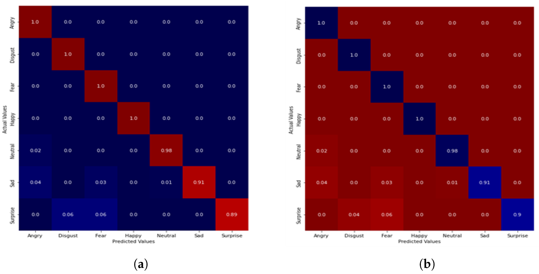
A normalized confusion matrix which depicts a holistic insight of various results obtained from our experiments with different classifiers is shown in Figure 3, Figure 4 and Figure 5, respectively. Looking at the confusion matrix, for the TESS dataset with the MLP classifier, 100% accuracy was recorded for angry, disgust, fear and happy emotion, while the surprise emotion yielded the lowest accuracy of 89%, and others were above 90%. With the SVM classifier, the minimum accuracy increased to 90%.

Figure 4. Confusion matrix of emotion classification on TESS dataset. (a) DCNN-NCA-MLP. (b) CNN-NCA-SVM.

Figure 5. Confusion matrix of emotion classification on the EMO-DB dataset. (a) DCNN-NCA-MLP. (b) CNN-NCA-SVM.

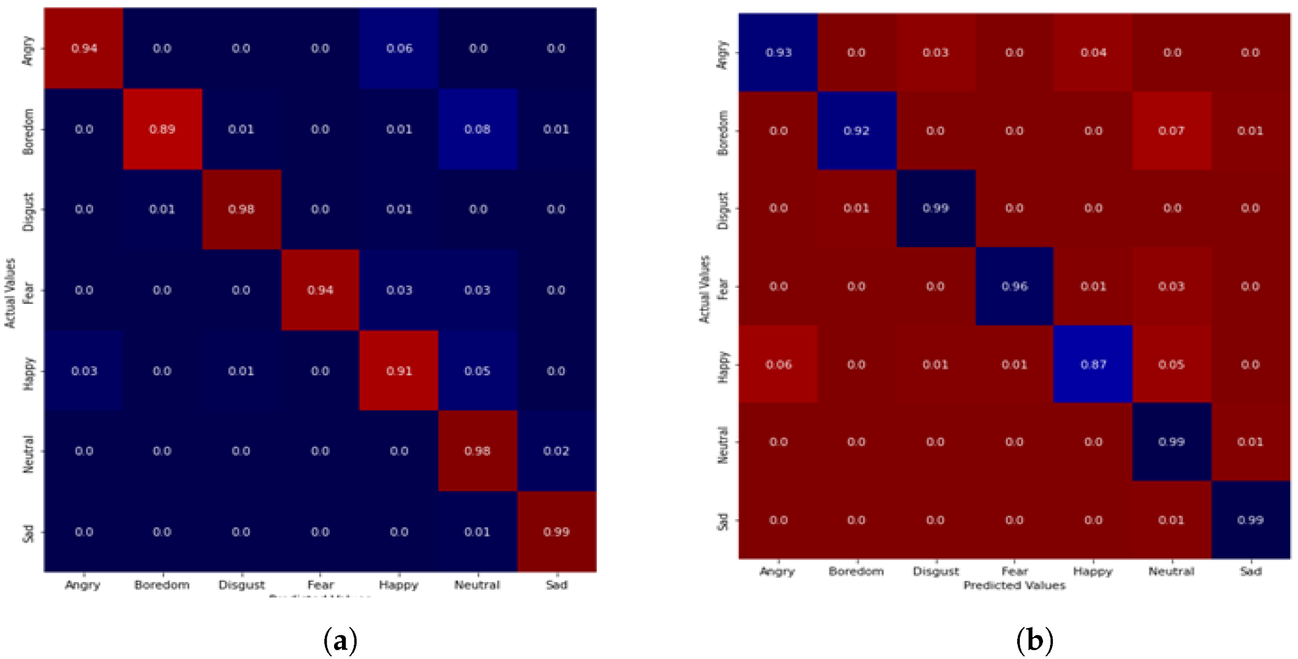
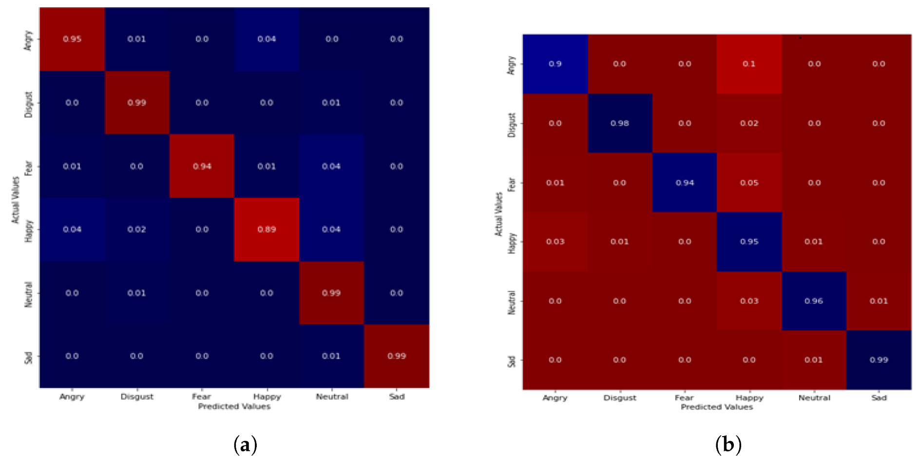
On the EMO-DB dataset, our model achieved 94%, 89%, 98%, 94%, 91%, 98% and 99% accuracy in classification for angry, boredom, disgust, fear, happy, neutral and sad emotion using the MLP classifier. When SVM was introduced, there was a slight improvement in recognition accuracy, as the three emotions (disgust, neutral and sad) recorded 99% accuracy while the happy emotion recorded the lowest accuracy of 87%. As with the combined dataset of TEES-EMO-DB, the highest accuracy of 99% was recorded for the sad, neutral and disgust emotions with the MLP classifier, while the happy emotion recorded the lowest accuracy of 87%, as depicted in Figure 6. For the SVM classifier, only the sad emotion produced the highest accuracy of 99%, while others were 90% and above.

Figure 6. Confusion matrix of emotion classification on TESS-EMODB dataset. (a) DCNN-NCA-MLP. (b) CNN-NCA-SVM.

As we analyze further, the classification report comprising accuracy, F1-score, specificity and sensitivity evaluation metrics was employed in order to fully grasp how efficient our proposed method performed in its discriminatory ability to learn features for speech emotion classification. As shown in Table 4, we achieved the highest accuracy of 97.2% on the TESS dataset with the SVM classifier, while the lowest accuracy of 94.3% was recorded from the EMO-DB dataset with the MLP classifier. The highest specificity and sensitivity of 100% was recorded with experiments on the two datasets for both classifiers, while 98.8% specificity was recorded on the combined dataset.

Table 4. Performance Evaluation.

MLP/SVM	TESS	EMO-DB	TESS-EMODB
F1-score (%)	97.20, 97.68	94.40, 94.40	95.70, 94.90
Sensitivity (%)	99.04, 100	100, 100	99.01, 98.95
Specificity (%)	98.90, 99.80	100, 100	100, 98.85

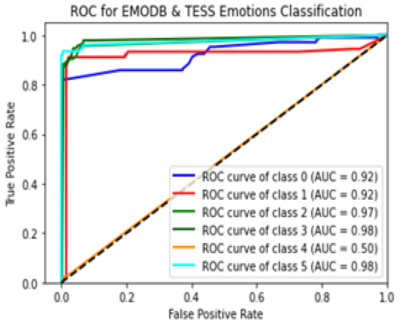
As with F1-score, we achieved a state-of-the-art result of 94.4%, 95.7% and 97%, respectively after evaluation on the three datasets. A return of operating curve (ROC) was adopted to present the graphical outlook of classification results of six emotions from the hybrid dataset. The ROC analysis result for six emotions on the combined dataset is illustrated in Figure 7. On the curve, each class represents an emotion: angry, sad, disgust, happy, fear and neutral with class 0 to 5, respectively. From the curve, the highest classification performance of Average Area Under the Curve (AUC) of 98% was achieved on classes 3 and 5 (neutral and disgust), while class 4 (fear) yielded the lowest AUC of 50%. However, none of the classes gave a classification outcome that is below the threshold (black dotted line). A chart indicating performance classification of emotion is also illustrated in Figure 8. The bars in represent experiments with MLP and SVM classifiers. From the chart, with SVM, five emotions comprising disgust, fear, happy, neutral and sad yielded accuracy results above 90%, while five emotions (sad, neutal, fear, disgust and angry) also yielded 90% and above accuracy.

Figure 7. ROC curve of classification.

Figure 8. Performance chart on TESS-EMODB with the two classifiers.

5.1. Performance Evaluation

The accuracy, specificity, and unweighted average recall (UAR) of our model are presented in Table 4. While accuracy measures the ratio of true emotion classified to all emotional classes in the dataset, specificity measures the ratio of actual emotion to predicted emotion. The evaluation result in this table showed the outcome of our work when a separate experiment using another classification algorithm (Random Forest) was conducted. The performance of our proposed method was compared with other studies in recent times, as indicated in Table 5, and our approach outperformed all of them in speech emotion classification. Additionally, a drastic reduction in complexity (at feature extraction and selection level) has been achieved, while the accuracy of emotion classification has been increased in our model as against what is obtained in the literature [2,38,39,40,41,42].

Table 5. Performance Evaluation.

Dataset	Reference	Methods	Reported Accuracy
TESS	(2018) [41]	DNN-GRU	89.96%
"	(2019) [42]	DNN-LSTM	70.00%
"	(2021) [2]	IMF-SVM, KNN	93.30%
"	(2022) [30]	LSTM-FCNN	86.02%
"	Proposed	DCNN-NCA-MLP	96.10%
EMO-DB	(2019) [43]	DCNN	80.79%
"	(2020) [44]	CNN-BiLSTM	85.50%
"	(2020) [22]	CNN	89.02%
"	(2021) [31]	DCNN-LSTM-Attention	87.86%
"	(2021) [20]	CNN-Attention	93.00%
"	(2021) [45]	LSTM-CNN	93.34%
"	Proposed	DCNN-NCA-MLP	94.90%

5.2. Performance Comparison

Our proposed model outperformed other existing methods when evaluated on the TESS and EMO-DB datasets, as shown in Table 3.

6. Conclusions and Future Work

In this work, a deep transfer learning approach with a feature selection algorithm that can select relevant features for speech emotion classification from a pool of extracted features through a deep convolutional neural network has been presented. It is obvious after a series of experiments have been carried out that the proposed method has improved accuracy and reduced the rate of misclassification as well as computational complexity using state-of-the-art emotional speech corpora. In achieving an optimum performance, the mel-spectrogram was extracted from raw speech signals through preprocessing and FFT. Thereafter, the mel-spectrogram was reshaped to match the requirement of the DCNN model for feature extraction. NCA feature selection was then applied in selecting the most salient and discriminating features that are relevant to emotion classification while reducing the workload of the classifier. With few hyperparameter tunning, our model achieved significant improvement in accuracy compared to existing methods as we carried out our experiment on the TESS, EMO-DB and combined (TESS+EMO-DB) dataset using two classifiers (MLP and SVM). Overall accuracies of 97.20%, 94.82% and 95.77% were obtained after we examined our method on TESS, EMO-DB and TESS+EMO-DB. The work has indicated that the proposed model is efficient for speech emotion classification. However, future experiments can be conducted using the cross-language speech corpus and testing with other classifiers to see their performance. We are also looking forward to adopting LSTM as an additional layer to our pretrained neural network and utilizing a multiple feature selection algorithm for an improved performance.