Figure 1.
Execution times for DAC, -O2 compilation flag; boxplot notation: medians, Q1 and Q3, max(Q1−1.5IQR, minimum) and min(Q3+1.5IQR, maximum) as well as potential outliers (+ for Docker, x for Host).
Figure 1.
Execution times for DAC, -O2 compilation flag; boxplot notation: medians, Q1 and Q3, max(Q1−1.5IQR, minimum) and min(Q3+1.5IQR, maximum) as well as potential outliers (+ for Docker, x for Host).
Figure 2.
Execution times for DAC, -O3 compilation flag; boxplot notation: medians, Q1 and Q3, max(Q1−1.5IQR, minimum) and min(Q3+1.5IQR, maximum) as well as potential outliers (+ for Docker, x for Host).
Figure 2.
Execution times for DAC, -O3 compilation flag; boxplot notation: medians, Q1 and Q3, max(Q1−1.5IQR, minimum) and min(Q3+1.5IQR, maximum) as well as potential outliers (+ for Docker, x for Host).
Figure 3.
Execution times for DAC, -O3 -march=native compilation flag; boxplot notation: medians, Q1 and Q3, max(Q1−1.5IQR, minimum) and min(Q3+1.5IQR, maximum) as well as potential outliers (+ for Docker, x for Host).
Figure 3.
Execution times for DAC, -O3 -march=native compilation flag; boxplot notation: medians, Q1 and Q3, max(Q1−1.5IQR, minimum) and min(Q3+1.5IQR, maximum) as well as potential outliers (+ for Docker, x for Host).
Figure 4.
Execution times for MasterSlave, -O2 compilation flag; boxplot notation: medians, Q1 and Q3, max(Q1−1.5IQR, minimum) and min(Q3+1.5IQR, maximum) as well as potential outliers (+ for Docker, x for Host).
Figure 4.
Execution times for MasterSlave, -O2 compilation flag; boxplot notation: medians, Q1 and Q3, max(Q1−1.5IQR, minimum) and min(Q3+1.5IQR, maximum) as well as potential outliers (+ for Docker, x for Host).
Figure 5.
Execution times for MasterSlave, -O3 compilation flag; boxplot notation: medians, Q1 and Q3, max(Q1−1.5IQR, minimum) and min(Q3+1.5IQR, maximum) as well as potential outliers (+ for Docker, x for Host).
Figure 5.
Execution times for MasterSlave, -O3 compilation flag; boxplot notation: medians, Q1 and Q3, max(Q1−1.5IQR, minimum) and min(Q3+1.5IQR, maximum) as well as potential outliers (+ for Docker, x for Host).
Figure 6.
Execution times for MasterSlave, -O3 -march=native compilation flag; boxplot notation: medians, Q1 and Q3, max(Q1−1.5IQR, minimum) and min(Q3+1.5IQR, maximum) as well as potential outliers (+ for Docker, x for Host).
Figure 6.
Execution times for MasterSlave, -O3 -march=native compilation flag; boxplot notation: medians, Q1 and Q3, max(Q1−1.5IQR, minimum) and min(Q3+1.5IQR, maximum) as well as potential outliers (+ for Docker, x for Host).
Figure 7.
Execution times for SPMD, -O2 compilation flag; boxplot notation: medians, Q1 and Q3, max(Q1−1.5IQR, minimum) and min(Q3+1.5IQR, maximum) as well as potential outliers (+ for Docker, x for Host).
Figure 7.
Execution times for SPMD, -O2 compilation flag; boxplot notation: medians, Q1 and Q3, max(Q1−1.5IQR, minimum) and min(Q3+1.5IQR, maximum) as well as potential outliers (+ for Docker, x for Host).
Figure 8.
Execution times for SPMD, -O3 compilation flag; boxplot notation: medians, Q1 and Q3, max(Q1−1.5IQR, minimum) and min(Q3+1.5IQR, maximum) as well as potential outliers (+ for Docker, x for Host).
Figure 8.
Execution times for SPMD, -O3 compilation flag; boxplot notation: medians, Q1 and Q3, max(Q1−1.5IQR, minimum) and min(Q3+1.5IQR, maximum) as well as potential outliers (+ for Docker, x for Host).
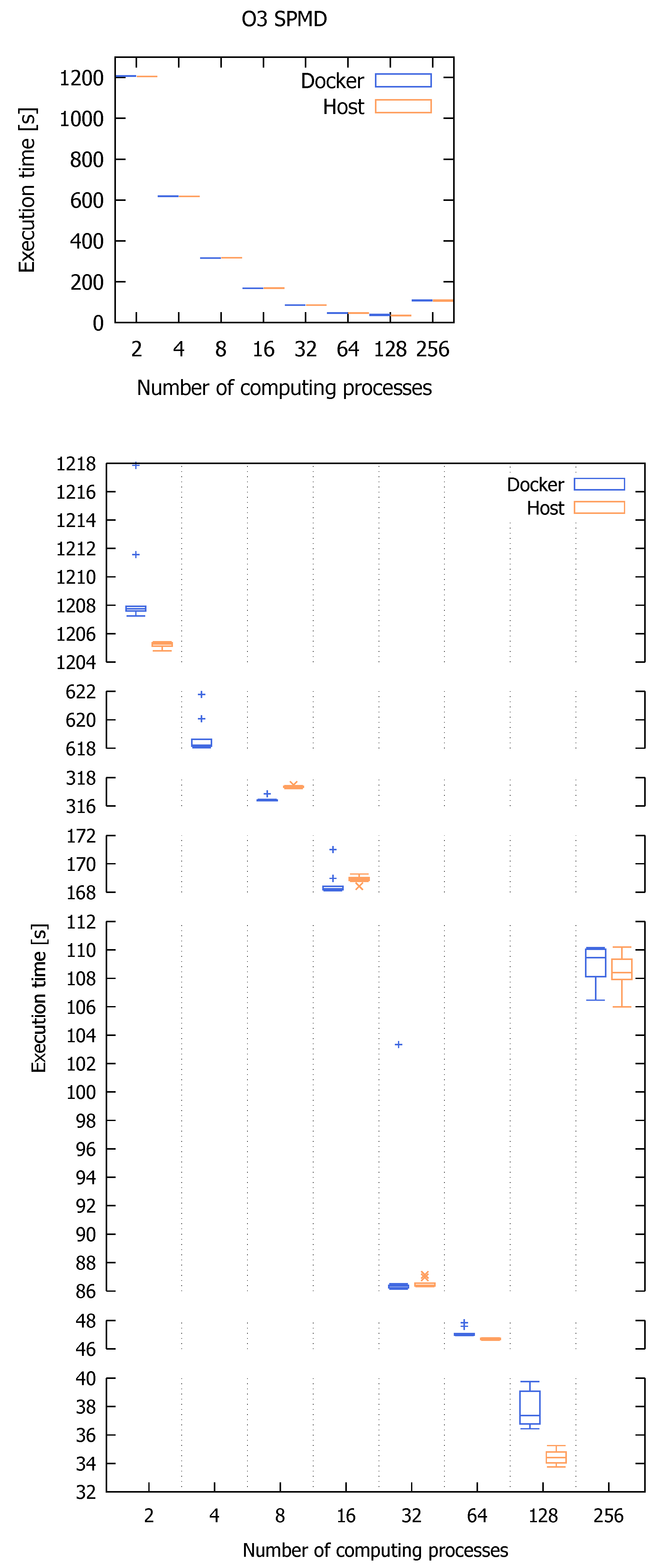
Figure 9.
Execution times for SPMD, -O3 -march=native compilation flag; boxplot notation: medians, Q1 and Q3, max(Q1−1.5IQR, minimum) and min(Q3+1.5IQR, maximum) as well as potential outliers (+ for Docker, x for Host).
Figure 9.
Execution times for SPMD, -O3 -march=native compilation flag; boxplot notation: medians, Q1 and Q3, max(Q1−1.5IQR, minimum) and min(Q3+1.5IQR, maximum) as well as potential outliers (+ for Docker, x for Host).
Figure 10.
Execution times for DAC, for better of Docker and host versions; boxplot notation: medians, Q1 and Q3, max(Q1−1.5IQR, minimum) and min(Q3+1.5IQR, maximum) as well as potential outliers (+ for O2, x for O3, * for O3_native).
Figure 10.
Execution times for DAC, for better of Docker and host versions; boxplot notation: medians, Q1 and Q3, max(Q1−1.5IQR, minimum) and min(Q3+1.5IQR, maximum) as well as potential outliers (+ for O2, x for O3, * for O3_native).
Figure 11.
Execution times for MasterSlave, for better of Docker and host versions; boxplot notation: medians, Q1 and Q3, max(Q1−1.5IQR, minimum) and min(Q3+1.5IQR, maximum) as well as potential outliers (+ for O2, x for O3, * for O3_native).
Figure 11.
Execution times for MasterSlave, for better of Docker and host versions; boxplot notation: medians, Q1 and Q3, max(Q1−1.5IQR, minimum) and min(Q3+1.5IQR, maximum) as well as potential outliers (+ for O2, x for O3, * for O3_native).
Figure 12.
Execution times for SPMD, for better of Docker and host versions; boxplot notation: medians, Q1 and Q3, max(Q1−1.5IQR, minimum) and min(Q3+1.5IQR, maximum) as well as potential outliers (+ for O2, x for O3, * for O3_native).
Figure 12.
Execution times for SPMD, for better of Docker and host versions; boxplot notation: medians, Q1 and Q3, max(Q1−1.5IQR, minimum) and min(Q3+1.5IQR, maximum) as well as potential outliers (+ for O2, x for O3, * for O3_native).
Figure 13.
Speed-up execution time of programs for computing processes.
Figure 13.
Speed-up execution time of programs for computing processes.
Figure 14.
Host and Docker comparison of execution times; orange points denote the overhead of Docker while blue points correspond to minimally better Docker execution times.
Figure 14.
Host and Docker comparison of execution times; orange points denote the overhead of Docker while blue points correspond to minimally better Docker execution times.
Figure 15.
Hardware counters for DAC program with -O2 compilation parameter; boxplot notation: medians, Q1 and Q3, max(Q1−1.5IQR, minimum) and min(Q3+1.5IQR, maximum) as well as potential outliers (+ for Docker, x for Host).
Figure 15.
Hardware counters for DAC program with -O2 compilation parameter; boxplot notation: medians, Q1 and Q3, max(Q1−1.5IQR, minimum) and min(Q3+1.5IQR, maximum) as well as potential outliers (+ for Docker, x for Host).
Figure 16.
Hardware counters for MasterSlave program with -O3 and -march=native compilation parameters (slave node); boxplot notation: medians, Q1 and Q3, max(Q1−1.5IQR, minimum) and min(Q3+1.5IQR, maximum) as well as potential outliers (+ for Docker, x for Host).
Figure 16.
Hardware counters for MasterSlave program with -O3 and -march=native compilation parameters (slave node); boxplot notation: medians, Q1 and Q3, max(Q1−1.5IQR, minimum) and min(Q3+1.5IQR, maximum) as well as potential outliers (+ for Docker, x for Host).
Figure 17.
Hardware counters for SPMD program with -O3 and -march=native compilation parameters; boxplot notation: medians, Q1 and Q3, max(Q1−1.5IQR, minimum) and min(Q3+1.5IQR, maximum) as well as potential outliers (+ for Docker, x for Host).
Figure 17.
Hardware counters for SPMD program with -O3 and -march=native compilation parameters; boxplot notation: medians, Q1 and Q3, max(Q1−1.5IQR, minimum) and min(Q3+1.5IQR, maximum) as well as potential outliers (+ for Docker, x for Host).
Figure 18.
Network bandwidth between nodes for selected size of data; boxplot notation: medians, Q1 and Q3, max(Q1−1.5IQR, minimum) and min(Q3+1.5IQR, maximum) as well as potential outliers (+ for Docker, x for Host).
Figure 18.
Network bandwidth between nodes for selected size of data; boxplot notation: medians, Q1 and Q3, max(Q1−1.5IQR, minimum) and min(Q3+1.5IQR, maximum) as well as potential outliers (+ for Docker, x for Host).
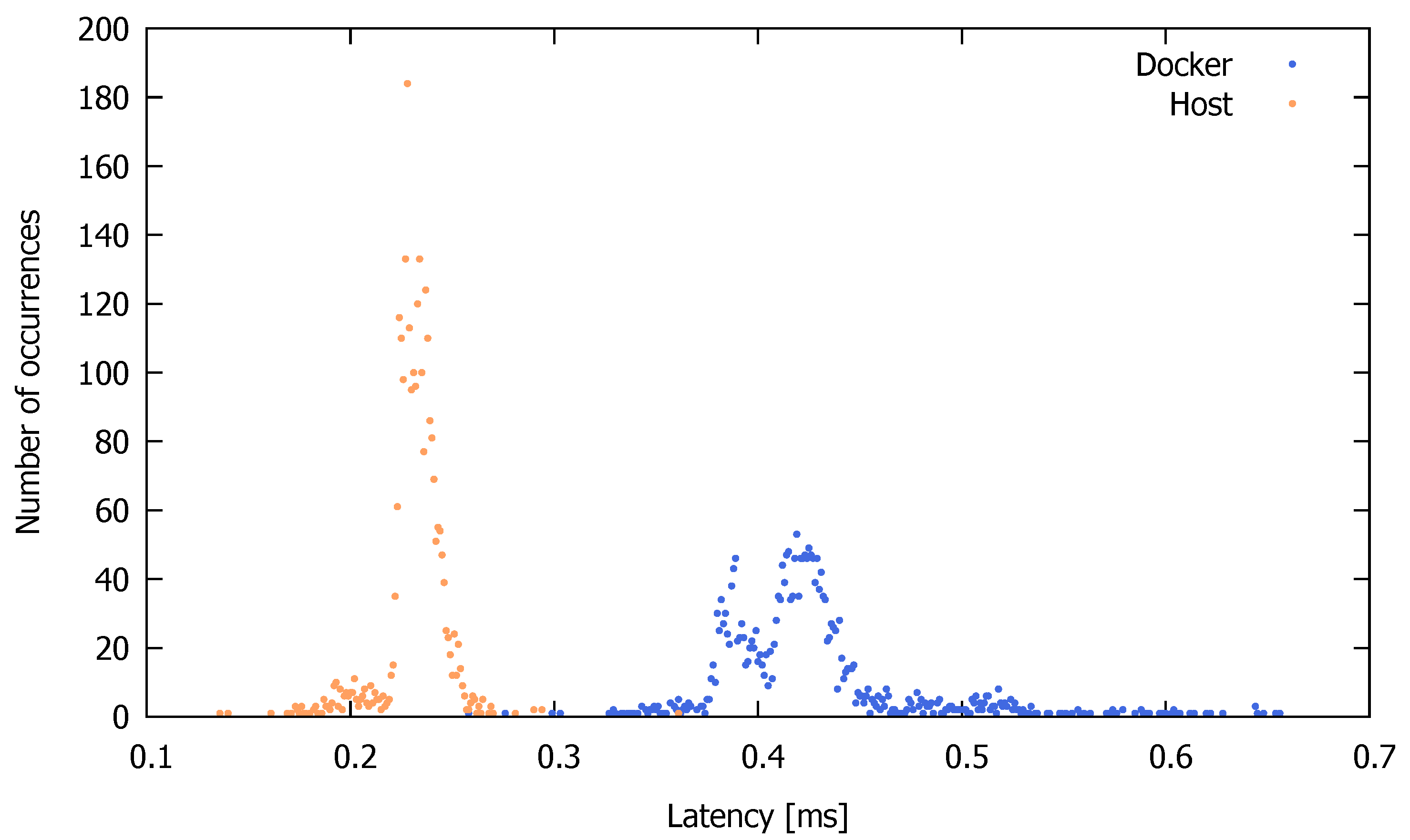
Figure 19.
Communication latency between nodes for Docker and Host.
Figure 19.
Communication latency between nodes for Docker and Host.
Table 1.
Median execution times for DAC.
Table 1.
Median execution times for DAC.
| Compilation | Runtime | Median Execution Time for Computing Processes [s] |
|---|
| Parameter | Machine | 2 | 4 | 8 | 16 | 32 | 64 | 128 | 256 |
|---|
| O2 | Docker | 267.60 | 137.01 | 69.10 | 34.93 | 18.18 | 10.22 | 10.96 | 10.73 |
| Host | 267.66 | 137.28 | 69.18 | 35.06 | 18.01 | 9.56 | 9.78 | 9.47 |
| O3 | Docker | 267.65 | 137.04 | 69.13 | 34.93 | 18.18 | 10.23 | 10.99 | 10.70 |
| Host | 267.79 | 137.32 | 69.21 | 35.04 | 18.01 | 9.58 | 9.80 | 9.41 |
| O3_native | Docker | 305.70 | 156.49 | 78.85 | 39.81 | 20.62 | 11.45 | 9.58 | 10.91 |
| Host | 305.91 | 156.78 | 78.93 | 39.92 | 20.45 | 10.79 | 9.86 | 9.42 |
Table 2.
Median execution times for MasterSlave.
Table 2.
Median execution times for MasterSlave.
| Compilation | Runtime | Median Execution Time for Computing Processes [s] |
|---|
| Parameter | Machine | 2 | 4 | 8 | 16 | 32 | 64 | 128 | 256 |
|---|
| O2 | Docker | 295.36 | 151.74 | 76.59 | 38.82 | 20.22 | 11.78 | 12.30 | 14.67 |
| Host | 288.87 | 149.46 | 75.21 | 38.21 | 19.97 | 10.86 | 11.57 | 13.09 |
| O3 | Docker | 295.34 | 151.74 | 76.59 | 38.84 | 20.21 | 12.43 | 12.28 | 14.61 |
| Host | 288.77 | 149.43 | 75.27 | 38.22 | 19.95 | 11.47 | 11.55 | 13.02 |
| O3_native | Docker | 280.92 | 144.18 | 72.86 | 36.95 | 19.28 | 11.28 | 12.04 | 14.52 |
| Host | 280.90 | 144.22 | 72.93 | 36.99 | 19.15 | 10.48 | 11.30 | 12.83 |
Table 3.
Median execution times for SPMD.
Table 3.
Median execution times for SPMD.
| Compilation | Runtime | Median Execution Time for Computing Processes [s] |
|---|
| Parameter | Machine | 2 | 4 | 8 | 16 | 32 | 64 | 128 | 256 |
|---|
| O2 | Docker | 1215.24 | 621.56 | 318.22 | 168.88 | 86.56 | 47.16 | 38.80 | 108.13 |
| Host | 1206.62 | 618.34 | 317.70 | 169.03 | 86.47 | 46.72 | 33.32 | 108.84 |
| O3 | Docker | 1207.75 | 618.21 | 316.42 | 168.23 | 86.35 | 47.00 | 37.38 | 109.46 |
| Host | 1205.28 | 617.70 | 317.32 | 168.92 | 86.40 | 46.70 | 34.41 | 108.41 |
| O3_native | Docker | 1206.68 | 617.46 | 316.04 | 167.78 | 86.04 | 46.87 | 38.86 | 109.30 |
| Host | 1204.94 | 617.45 | 317.19 | 168.80 | 86.38 | 46.73 | 33.70 | 108.84 |
Table 4.
Median execution time for each parameters, programs and computing processes.
Table 4.
Median execution time for each parameters, programs and computing processes.
| Computing | Program | Median Execution Time [s] |
|---|
| Processes | O2 | O3 | O3_native |
|---|
| 1 | DAC | 522.020 | 523.520 | 598.110 |
| MasterSlave | 564.610 | 564.354 | 548.795 |
| SPMD | 2361.605 | 2358.880 | 2357.340 |
| 2 | DAC | 267.600 | 267.650 | 305.700 |
| MasterSlave | 288.874 | 288.771 | 280.902 |
| SPMD | 1206.615 | 1205.275 | 1204.935 |
| 4 | DAC | 137.005 | 137.040 | 156.490 |
| MasterSlave | 149.458 | 149.430 | 144.180 |
| SPMD | 618.340 | 617.695 | 617.445 |
| 8 | DAC | 69.100 | 69.130 | 78.850 |
| MasterSlave | 75.213 | 75.269 | 72.860 |
| SPMD | 317.701 | 316.415 | 316.040 |
| 16 | DAC | 34.930 | 34.930 | 39.810 |
| MasterSlave | 38.211 | 38.219 | 36.950 |
| SPMD | 168.875 | 168.230 | 167.775 |
| 32 | DAC | 18.005 | 18.010 | 20.450 |
| MasterSlave | 19.971 | 19.946 | 19.150 |
| SPMD | 86.470 | 86.345 | 86.035 |
| 64 | DAC | 9.560 | 9.580 | 10.790 |
| MasterSlave | 10.862 | 11.474 | 10.480 |
| SPMD | 46.723 | 46.702 | 46.732 |
| 128 | DAC | 9.780 | 9.797 | 9.575 |
| MasterSlave | 11.570 | 11.550 | 11.293 |
| SPMD | 33.322 | 34.412 | 33.704 |
| 256 | DAC | 9.472 | 9.408 | 9.416 |
| MasterSlave | 13.094 | 13.022 | 12.834 |
| SPMD | 108.130 | 108.406 | 108.850 |
Table 5.
Execution time factor for parameters (results of p function).
Table 5.
Execution time factor for parameters (results of p function).
| Program | | | |
|---|
| DAC | 0.9985 | 0.8756 | 0.8769 |
| MasterSlave | 0.9998 | 1.0304 | 1.0306 |
| SPMD | 1.0012 | 1.0020 | 1.0008 |
Table 6.
The best compilation flag for each program.
Table 6.
The best compilation flag for each program.
| Program | The Best Compilation Flag |
|---|
| DAC | O2 |
| MasterSlave | O3_native |
| SPMD | O3_native |
Table 7.
Speed-up execution time of programs for computing processes.
Table 7.
Speed-up execution time of programs for computing processes.
| Program | Runtime | Speedup for Computing Processes [s] |
|---|
| Machine | 1 | 2 | 4 | 8 | 16 | 32 | 64 | 128 | 256 |
|---|
| DAC | Docker | 1.00 | 1.95 | 3.81 | 7.55 | 14.94 | 28.71 | 51.08 | 47.65 | 48.65 |
| Host | 1.00 | 1.95 | 3.81 | 7.56 | 14.91 | 29.04 | 54.69 | 53.47 | 55.20 |
| MasterSlave | Docker | 1.00 | 1.95 | 3.81 | 7.53 | 14.85 | 28.47 | 48.67 | 45.60 | 37.80 |
| Host | 1.00 | 1.95 | 3.81 | 7.53 | 14.84 | 28.67 | 52.39 | 48.62 | 42.78 |
| SPMD | Docker | 1.00 | 1.96 | 3.83 | 7.49 | 14.11 | 27.51 | 50.50 | 60.91 | 21.66 |
| Host | 1.00 | 1.96 | 3.82 | 7.43 | 13.97 | 27.29 | 50.44 | 69.94 | 21.66 |
Table 8.
Host and Docker comparison of median execution times.
Table 8.
Host and Docker comparison of median execution times.
| (CP) | DAC | MasterSlave | SPMD |
|---|
| (A) | (B) | (C) | (Sf) | (A) | (B) | (C) | (Sf) | (A) | (B) | (C) | (Sf) |
|---|
| 1 | 0.85 | D | 0.16 | 1.0000 | 0.19 | D | 0.04 | 0.9996 | 9.71 | H | 0.41 | 1.0041 |
| 2 | 0.06 | D | 0.02 | 0.9986 | 0.01 | H | 0.00 | 1.0000 | 1.74 | H | 0.14 | 1.0014 |
| 4 | 0.28 | D | 0.20 | 1.0004 | 0.04 | D | 0.03 | 0.9997 | 0.01 | H | 0.00 | 1.0000 |
| 8 | 0.08 | D | 0.11 | 0.9995 | 0.07 | D | 0.10 | 0.9990 | 1.15 | D | 0.36 | 0.9964 |
| 16 | 0.13 | D | 0.37 | 1.0021 | 0.04 | D | 0.10 | 0.9990 | 1.03 | D | 0.61 | 0.9939 |
| 32 | 0.17 | H | 0.97 | 0.9888 | 0.13 | H | 0.65 | 1.0065 | 0.34 | D | 0.40 | 0.9960 |
| 64 | 0.66 | H | 6.90 | 0.9339 | 0.80 | H | 7.59 | 1.0759 | 0.14 | H | 0.30 | 1.0030 |
| 128 | 1.18 | H | 12.02 | 0.8913 | 0.74 | H | 6.58 | 1.0658 | 5.16 | H | 15.30 | 1.1530 |
| 256 | 1.26 | H | 13.29 | 0.8813 | 1.69 | H | 13.14 | 1.1314 | 0.45 | H | 0.41 | 1.0041 |
Table 9.
Better compiler version using Docker.
Table 9.
Better compiler version using Docker.
| Computing | Program |
|---|
| Processes | DAC | MasterSlave | SPMD |
|---|
| 1 | V9 (17.26%) | V9 (0.17%) | V9 (0.98%) |
| 2 | V9 (17.00%) | V9 (0.15%) | V9 (1.00%) |
| 4 | V9 (16.98%) | V9 (0.14%) | V9 (0.90%) |
| 8 | V9 (16.85%) | V9 (0.10%) | V9 (1.14%) |
| 16 | V9 (16.67%) | V7 (0.15%) | V9 (1.04%) |
| 32 | V9 (15.89%) | V7 (0.73%) | V9 (0.94%) |
| 64 | V9 (14.26%) | V7 (2.48%) | V9 (0.67%) |
Table 10.
Minimum, maximum and median communication latency between nodes for Docker and Host.
Table 10.
Minimum, maximum and median communication latency between nodes for Docker and Host.
| Runtime | Latency [s] |
|---|
| Machine | Min | Max | Median |
|---|
| Docker | 0.258 | 0.656 | 0.419 |
| Host | 0.136 | 0.361 | 0.232 |


