Accelerated Inference of Face Detection under Edge-Cloud Collaboration

Abstract

Model compression makes it possible to deploy face detection models on devices with limited computing resources. Edge–cloud collaborative inference, as a new paradigm of neural network inference, can significantly reduce neural network inference latency. Inspired by these two techniques, this paper adopts a two-step acceleration strategy for the CenterNet model. Firstly, the model pruning method is used to prune the convolutional layer and the deconvolutional layer to obtain a preliminary acceleration effect. Secondly, the neural network is segmented by the optimizer to make full use of the computing resources on the edge and the cloud to further accelerate the inference of the neural network. In the first strategy, we achieve a 62.12% reduction in inference latency compared to the state-of-the-art object detection model Blazeface. Additionally, with a two-step speedup strategy, our method is only 26.5% of the baseline when the bandwidth is 500 kbps.

1. Introduction

Face detection is widely used in today’s industries, and faces have large visual errors in different backgrounds, which makes face detection more difficult. Scholars have proposed lots of models successively, such as PyramidBox [1], TinaFace [2], SRN [3], and so on. They achieved decent performance in accuracy. However, in edge devices with limited computing resources, such as mobile phones, Raspberry Pi, and other embedded devices with insufficient computing resources, when deploying large models, there will be problems such as high inference delay, excessive energy consumption, and memory overflow. In addition, in recent years, some scholars have made contributions to the application of face models [4] and facial feature data [5]. For example, Deng et al. [4] proposed an MFCosface to solve the problem of low facial recognition rate during the epidemic.

On the one hand, the appearance of model compression [2,6,7,8,9,10] alleviates this problem to a certain extent. Model pruning, as an effective means of model compression, can ensure the accuracy of the model and reduce the FLOPs of the model. Han et al. [11] obtained a sparse weight matrix by retraining the network by setting the weights below the threshold to 0 and repeating this process. However, this approach is mostly used in CNN image classifiers and is rarely used in other fields. On the other hand, edge–cloud collaborative inference, as a new neural network inference paradigm, can effectively reduce the neural network inference delay. It divides a large neural network into two parts: one part is deployed on edge devices, and the other part, which usually has a larger scale and higher computational load, is deployed on cloud servers. Neurosurgeon [12] used this paradigm to divide the middle layer of the neural network model to reduce the communication delay, thereby speeding up the end-to-end reasoning speed. Inspired by these two aspects, this paper makes full use of the characteristics of both to perform two-step acceleration processing on the deep neural network model to reduce the end-to-end inference delay of the model. The overall framework of the algorithm is shown in Figure 1. It mainly includes three phases: cloud training phase, optimization phase, and collaborative inference phase.

Cloud training phase. At the beginning of the training phase, a target detection model with strong generalization ability is obtained through the training dataset. After that, all layers of the model are decoupled and redundantly analyzed, and the convolutional and deconvolutional layers are pruned through ${\mathrm{L}}_1$ regularization sorting and predefined thresholds. The pruning operation may inevitably destroy the generalization ability of the original model, then use the global fine-tuning strategy to restore the accuracy of the model, so that a simplified model with less computation and less loss of accuracy can be obtained.

Optimization phase. The optimizer selects the best split point of the model under the current dynamic bandwidth to maximize the performance of the model and speed up the delay of end-to-end inference. It mainly relies on three inputs: (1) the dynamic bandwidth and delayed demand; (2) the compressed model through cloud training, which requires much fewer computing resources than the original model; (3) the relational mapping table is the pre-split point and the inference latency between different devices by testing in the actual operation. In addition, the specific implementation of the optimizer algorithm is detailed in Section 3.

Collaborative inference phase. The model is divided according to the best split point. One part that requires fewer computing resources is deployed on the edge, and the other part requires a large amount of computing to be deployed on the cloud server.

The remainder of the paper is structured as follows: Section 2 provides background and related technical information. Section 3 provides a more detailed design of our algorithm. In Section 4, we give the test environment on the actual hardware and compare the experimental results of different approaches. Section 5 gives the summary of our paper and future work.

2. Related Work

2.1. Face Detection Models

Face detection models have been widely researched and applied in the past decade. Early face detection models used artificial classifiers to detect faces in the form of sliding windows. Violia et al. [13] used the AdaBoost algorithm to train face classifiers, and then more effective classifiers [14,15] were created. However, none of these methods can achieve end-to-end training and cannot achieve satisfactory results in accuracy. At this stage, face detection models are all based on convolutional neural networks (CNNs). Many excellent models have been proposed in order to solve the problems in the field of face detection, such as scale, posture, etc. These models include HAMBox [16], DSFD [17], TinaFace [2], CenterNet [18], etc. However, these models generally require a large amount of computation, which is not friendly to deploying models on devices with limited computing resources. Some works have also made efforts to reduce FLOPs, but the generalization ability of the model is not ideal, such as FaceBoxes [19]. How to balance model size and its accuracy has always been a difficult problem to deploy models on resource-constrained devices.

2.2. Model Pruning

Model pruning can be divided into structured pruning and unstructured pruning. Unstructured pruning is the removal of unimportant weights, which do not change the structure of the network. Structured pruning is the removal of various structured parts, such as channels, filters, or layers. Channel pruning decides whether to delete a layer by judging the importance of the layer. Different important measures include the ${\mathrm{L}}_1$ norm [6], LASSO regression [7], and so on. Similar to channel pruning, filter pruning removes redundant filters [8,9], thereby reducing the computational complexity of the model. Additionally, layer pruning is used for static block pruning [10] as well as data-dependent reasoning [20]. In model pruning, the selection of model generalization ability and pruning rate has always been a concern of researchers.

2.3. Model Partition

To make full use of computing resources at the edge and cloud, some recent works offload DNN inference tasks from local to cloud servers [12,21,22,23]. Neurosurgeon [12] firstly determined a DNN partition point and placed the partition point on the edge side in the shallow layer, and the partition point in the deep layer of the cloud, to achieve the purpose of joint reasoning. DDNN [22] applied a similar principle to map DNNs into a distributed computing hierarchy. DDNN is capable of accommodating DNN inference in the cloud, while also allowing fast, localized inference using shallow parts of neural networks at the edge and end devices. Branchy-GNN [23] utilized an edge computing platform for efficient graph neural network (GNN)-based point cloud processing and added branches to the network structure for an early exit at the edge. In addition, they adopted learning-based joint source–channel coding (JSCC) for intermediate feature compression to reduce communication overhead.

To complete face detection tasks on resource-constrained devices, some works introduced model pruning strategies into face detection models, but they are all based on traditional cloud-based inference or edge-based inference. For example, PruneFaceDet [24] used a network pruning method to prune the EagleEye [25] model to reduce the model size. However, this method was based on the traditional reasoning method. In contrast, our method decouples the model in multiple steps, makes full use of the mutual influence of model compression and model partition, and combines the computing resources of the edge and the cloud to achieve the purpose of accelerating the model inference speed.

3. Proposed Method

3.1. Research Motivation

The CenterNet object detection model is based on the keypoint estimation network, finds the center of the object, and obtains other properties of the object through regression. As a typical representative of anchor-free, this model has achieved good results in both speed and accuracy and is end-to-end differentiable. In addition, there is no need to perform any subsequent processing of non-maximum suppression (NMS), which saves computing resources. This paper performs further research on the CenterNet model. Through experiments, it is found that, as shown in Figure 2, the amount of computation in each layer is different, and the most important thing is that the main amount of computation is concentrated in the deconvolution layer [26] (deconv). The previous work is to prune the convolutional layer or other model compression processing, and rarely prune the deconvolutional layer. Based on this, this paper analyzes the redundant features of the convolutional and deconvolutional layers in CenterNet, and finds that these layers can be further pruned and compressed to reduce the amount of computation and parameters of the model.

Interestingly, as the network deepens, the output size of each layer is different. As shown in Figure 3, the smallest output is reached before the deconvolution layer. Combined with the research in Figure 2, it can be found that there is a possibility of partition in the CenterNet because the output data of the shallow layer are large but the amount of computation is small, and the output data of the deep layer are small but the amount of computation is large; that is to say, the neural network model is divided into two parts. The shallow part with a small amount of calculation and a large output is placed on the edge device for calculation, and the deep part with a large amount of calculation and a small output is placed on the server for calculation. The computing resources of the edge device and the server are combined to minimal network overhead speeding up inference for face recognition in object detection tasks. Combining the findings of Figure 2 and Figure 3, this paper will adopt a double-layer acceleration structure. The first step of acceleration is through pruning the convolutional layer and deconvolution, and the second step of acceleration is through the best split point, joint cloud–edge computing resources to reduce end-to-end delay.

3.2. ${\mathrm{L}}_1$ Weight Pruning

The pruning strategy can effectively reduce the amount of calculation and parameters of the model. The ${\mathrm{L}}_1$ weight pruning strategy is mainly divided into the following parts, as shown in Figure 4. Step 1: train the model. With the training dataset, the model with the highest accuracy is selected from multiple training units. In addition, this paper will adjust the hyperparameters before and after training to obtain better model training accuracy. Step 2: ${\mathrm{L}}_1$ weight pruning. The selected models are decoupled layer by layer and the weights are sorted by ${\mathrm{L}}_1$ regularization. This method only operates on the weights of the convolutional layers and does not involve the offset value (bias) of the weights. ${\mathrm{L}}_1$ regularization can judge the importance of weight parameters, and delete the weights below the threshold through the set threshold. The ${\mathrm{L}}_1$ norm is the sum of the weights of the elements in the vector. In the optimization solution, the ${\mathrm{L}}_1$ norm is the optimal convex approximation of the ${\mathrm{L}}_0$ norm. Therefore, this paper adopts the ${\mathrm{L}}_1$ regularization method [26] to judge the importance of weights. Step 3: global fine-tuning. For the pruned model, including pruning of convolutional and deconvolutional layers, see the next section for the details of deconvolution pruning. Then, the generalization ability of the model will inevitably decline. A global fine-tuning approach is adopted to restore the accuracy of the model through the same training set.

3.3. Deconvolution Pruning

In the CenterNet structure, the deconvolution layer obtains high-resolution feature layers by upsampling the feature data extracted by the backbone network. In addition, this layer can be similar to upsampling methods (bilinear interpolation [11,27], etc.), but upsampling methods cannot be learned and the model cannot be trained end-to-end.

Generally, for a convolutional neural network with L convolutional layers, input tensor is $X^l\in {\mathbb{R}}^{c^l·h_{in}^l·w_{in}^l}$, output tensor is $Y^l\in {\mathbb{R}}^{c^l·h_{out}^l·w_{out}^l}$, and weight tensor is $W^l\in {\mathbb{R}}^{n^l·c^l·k^l·k^l}$, where $n^l$ and $c^l$ represent the number of input channels and output channels, $k^l·k^l$ is filter size, and l is the layer index. The deconvolution operation can be expressed as Equation (1).

$$X={\left(W^l\right)}^{\mathrm{T}}\otimes {\mathrm{Y}}^l$$

(1)

Here, ⊗ is represented as a convolutional layer operation. In this way, it can be found that the deconvolution operation is the inverse process of the convolution operation, but the deconvolution can only restore the size of the tensor, not the value in the tensor. Thus, there is redundancy in the deconvolution and the pruning operation can be performed. In addition, the bias operation is omitted in the formula. ${\overline{W}}^l\in {\mathbb{R}}^{{\overline{n}}^l·c^l·k^l·k^l}$ indicates the weight after pruning. Therefore, the pruning process can be expressed as a function ${\overline{W}}^l=F\left(W^l,percent\right)$. The relationship between the input channels is shown in Equation (2) and the p is expressed as the pruning rate. It is worth noting that before the pruning operation, this algorithm sorts all the weights, and the sorting method is also ${\mathrm{L}}_1$ regularization.

$${\overline{n}}^l=n^l·p$$

(2)

In the deconvolution operation, the size relationship between the input and output is as shown in Equation (3). $s^l$ is the step of the deconvolution layer, $p^l$ is the pace of the layer. If you change the number of input channels, the natural number of output channels will also change.

$$c^l=s^l\left(n^l-1\right)-2p^l+k^l$$

(3)

3.4. Joint Optimization of Model Split Points and Bandwidth

In the optimization phase, the optimizer searches for dynamic split points based on the current bandwidth of edge devices through the reduced model in the cloud server training phase and acceptable latency requirements. Algorithm 1 gives the complete process. For the compressed CenterNet model with N pre-split points, this paper firstly establishes a relationship mapping table based on different split points and the computing resources of edge devices and cloud server devices. The relational mapping table will be transferred to the optimizer during the optimization phase. The relational mapping table takes a similar idea with Neurosurgeon [12] and Edgent [28] interlayer prediction models. This algorithm simplifies the operation in the experiment. According to the prior knowledge of the actual operation, a one-to-one correspondence is established between the interlayer running delay of different devices and the split point, and then the relationship mapping table is formed. In addition, the feature extraction network structure adopts the resnet residual network. In this paper, each residual block is regarded as a whole, and its prediction delay is the sum of the prediction delays of each layer, which simplifies the selection of split points. As for the layers before the first residual block, this paper also treats it as a whole, because after the maxpool pooling layer [29], the size of the output data is subject to change. Note that the relational mapping table needs to be tested. Once the relational mapping table is established, it becomes a simple linear index, and the decision-making speed is very fast.

Algorithm 1 The partition algorithm

Input: N: numbers of pre-partition points $\left\{L_i\left|i=1,2,\cdots ,N\right.\right\}$: numbers of layer before partition point $\left\{D_j\left|j=1,2,\cdots ,N\right.\right\}$: each layers output data size after partition point $f\left(L_j\right)$: relationship mapping table of different partition point B: current bandwidth $latency$: the target latency Output: Split point selection  //Procedure 1: for i = 1; i <= N; i++ do 2:     ${\mathrm{TM}}_i$ = $f_{mobile}\left(L_j\right)$ 3:     ${\mathrm{TU}}_i$ = ${\mathrm{D}}_i/\mathrm{B}$ 4:     ${\mathrm{TC}}_i$ = $f_{cloud}\left(L_j\right)$ 5:     T = ${{\sum }_{j=1}^{i}T{M}_i+{\sum }_{j=i+1}^{N}TC}_i+T{U}_i$ 6:     if T ≤ latency and T is min latency then 7:           return Selection of partition point 8:     else 9:           return NULL 10:     end if 11: end for

The optimization problem defined in (4) is actually to minimize the end-to-end inference latency. It consists of three parts: mobile Terminal execution delay ($T{M}_i$), transmission delay ($T{U}_i$), and cloud execution delay ($T{C}_i$). The delay of these three parts is affected by the dynamic split point, which is obtained by the split point algorithm we give. In short, we will adaptively find the best split point in the current state according to the delay requirements given by the user and the current network bandwidth to minimize the delay.

$$Z=\sum _{i=1}^{P-1}T{M}_i+T{U}_i+\sum _{\mathrm{i}=P}^{N}T{C}_i$$

(4)

4. Evaluation

4.1. Experiment Setup

4.1.1. Environment

In order to verify the feasibility and efficiency of the algorithm, this paper trains the compression model on the server and tests the compression performance on the server. In addition, the compressed model is further accelerated based on Tensort RT [30]. Finally, the NVIDIA JETSON NANO is used to simulate the edge device, the PC simulates the edge server, and the model is used for collaborative reasoning. The WonderShaper [31] tool is used to control the bandwidth on the edge device and the edge server. The server, NANO, and PC are all loaded with the Ubuntu 18.04 system, and the Pytorch [32] environment is built. The configuration details of the three are shown in

Table 1. Details of hardware resource configuration.

Component	Cloud Server	NVIDIA JETSON NANO	PC
GPU	Two NVIDIA GeForce RTX 3090	NVIDIA Maxwell w/128	NVIDIA Geforce GTX 1060
CPU	Intel(R) Xeon(R) silver 4210 CPU @ 2.20 GHz	quad-core ARM Cortex-A57 64-bit	Intel(R) Core (TM) i7-8750H CPU @ 2.20 GHz
Memory	128 GB DDR4	4 GB LPDDR4	16 GB DDR4

.

4.1.2. Dataset

This algorithm uses the open-source dataset WIDER FACE, which is the benchmark dataset for face detection. It contains 32,203 images and 393,703 labels, which cover scale, pose, and occlusion. Among them, the training set accounts for 40%, the validation set accounts for 10%, and the test set accounts for 50%. According to the difficulty of image detection, images are divided into three levels: easy, medium, and hard. Many tiny faces are located in medium and hard. In the experiment, this paper uses all the training sets to obtain a model with strong generalization ability and uses all the validation sets to evaluate the performance of the model.

4.1.3. Performance

(1) The average precision MAP (mean average precision) is an important indicator for evaluating the performance of target detection. It is the area of the curve (P–R curve) between precision and recall. The formulas for precision and recall are as follows. TP is the number of correctly detected detection frames, FP is the number of falsely detected detection frames, and FN is the number of undetected frames.

$$\mathrm{precision}=\frac{\mathrm{TP}}{\mathrm{TP}+\mathrm{FP}}$$

(5)

$$\mathrm{recall}=\frac{\mathrm{TP}}{\mathrm{TP}+\mathrm{FN}}$$

(6)

(2) Ms is an indicator to measure the model inference speed.

(3) Kbps is the network bandwidth, which measures the transmission capacity of the network.

4.2. Deconvolution Pruning Results

The CenterNet network is an end-to-end detection model based on center point regression. This algorithm uses the resnet residual network as the backbone network to extract the features of the input data and tests its performance on the WIDER FACE dataset. For the deconvolution layer, this algorithm tries to use the pruning strategy to remove redundant features and makes a comparison with the traditional pruning convolution layer, which is represented as backbone pruning in the table (see

Table 2. Comparison of different approaches for CNN inference.

Pruning Strategy	Compression Ratio	AP_Easy	AP_Medium	AP_Hard	FLOPs/GMAC	Parameter/M
Backbone pruning	1	83.635	79.481	79.481	40.15	15.815
	0.80	83.682	79.995	56.332	56.332	11.341
	0.60	81.636	77.014	53.785	33.576	7.81
Deconvolution pruning	1	83.635	79.481	54.748	40.15	15.815
	0.80	83.709	80.031	56.518	26.96	10.145
	0.60	81.965	77.983	53.812	16.331	5.777

for details). On the one hand, the AP values of three different indexes (easy, medium, hard) for different models in the WIDER FACE dataset are kept within a 2% accuracy loss compared to the model with a compression rate of 1. For the pruning model with a compression rate of 0.8, compared with the baseline, whether it is backbone pruning or deconvolution pruning, the AP value improved, and the hard class has the most obvious improvement. On the other hand, the AP value, the amount of calculation, and the number of parameters have different degrees of improvement under the same compression rate for backbone pruning and deconvolution pruning. In the experiments, the input resolution size is set to 3 × 512 × 512 when calculating FLOPs. For deconvolution pruning with a compression ratio of 0.6, compared with the baseline, not only is the loss of AP value kept within a reasonable range, but the amount of computation is also reduced by about 59.33%, and the number of parameters is reduced by 63.47%. The experimental results show that the deconvolution pruning algorithm can fully reduce the calculation amount and parameter amount of the CenterNet model, and has a good acceleration inference effect.

In addition, this algorithm compares other outstanding face detection models on the WIDER FACE dataset, Pyramidbox [1], S3FD [33], and SSH [34] (see

Table 3. Comparison of different models on the WIDER FACE dataset.

Model	AP_Easy	AP_Medium	AP_Hard	FLOPs/GMAC	Parameter/M
PyramidBox	92.6	92.0	86.2	236.58	57.18
S3FD	92.3	90.70	82.2	96.60	22.46
SSH	92.1	90.7	70.2	99.98	19.75
Ours	81.965	81.965	53.812	19.138	5.777

for details). For the sake of fairness, the validation datasets are all the validation datasets in the WIDER FACE dataset and the same input resolution is set to 3 × 640 × 480 when calculating FLOPs. Compared with the advanced face detection model, although this algorithm sacrifices the accuracy of the model, it greatly reduces the calculation amount and parameter amount of the model. Compared with the calculation amount of Pyramidbox, this algorithm is 8% of it, and the parameter amount is 10.1% of it. Through the experimental results in Table 2 and Table 3, deconvolution pruning can achieve a good balance between accuracy and model size.

4.3. Acceleration Effect on the Server

In order to test the effect of the first-layer acceleration of this algorithm, an inference speed test experiment was performed on the server. The server is equipped with two NVIDIA GeForce 3090s, and only one of the GPUs was used for the test. For the test dataset, 19 face images of different sizes with different detection difficulties were selected. Second, a single image was also selected as the test with a resolution of 3 × 512 × 512. Finally, the model was converted into a Tensort RT model, which is referred to as the TRT model in the table. For the inference delay of the model without TRT and the model with TRT, 19 face pictures of different sizes were used in the experiment, and the inference delay includes the data processing time of the 19 pictures, which is converted into a unified input size 3 × 512 × 512.

As shown in

Table 4. Inference speed of different pruning strategies on the server.

Pruning Strategy	Compression Ratio	NO TRT Inference Delay	TRT Inference Delay	TRT Load Delay	Per Image Delay
Backbone pruning	1	265.919 ms	145.392 ms	3287.6 ms	2.496 ms
	0.80	251.741 ms	140.882 ms	3066.7 ms	2.276 ms
	0.60	242.892 ms	135.738 ms	2674.7 ms	1.939 ms
Deconvolution pruning	1	265.919 ms	145.392 ms	3287.6 ms	2.496 ms
	0.80	221.656 ms	130.265 ms	2817.5 ms	1.955 ms
	0.60	198.333 ms	119.374 ms	2563.9 ms	1.451 ms

, the deconvolution pruning algorithm can speed up the processing time for the reduced model after compression pruning, whether it is a TRT model or a non-TRT model. In the inference delay of a single image, the deconvolution pruning model with a compression rate of 0.6 has an inference speed of only 1.434 milliseconds, which is nearly 41.87% faster than that of the model without any pruning processing. At the same time, the algorithm also reduces model load time. It can be seen that the first step acceleration strategy greatly reduces the inference delay of the model on the server.

4.4. Comparison of Different Input Resolutions

Input resolution is an important factor affecting inference latency. This section tests the inference latency of models with different pruning strategies at different resolutions. The test environment was performed on a GPU equipped with an NVIDIA GeForce 3090 [35]. Second, the input batch size was set to 1, and the final result was an average of 50 runs for testing accuracy. As shown in

Table 5. Inference latency at different input resolutions.

Pruning Strategy	Compression Ratio	3 × 320 × 240	3 × 320 × 240	3 × 1280 × 720
Backbone pruning	1	1.514 ms	2.657 ms	4.728 ms
	0.80	1.252 ms	2.387 ms	4.417 ms
	0.60	1.146 ms	2.239 ms	4.206 ms
Deconvolution pruning	1	1.514 ms	2.657 ms	4.728 ms
	0.80	1.071 ms	2.279 ms	3.810 ms
	0.60	0.891 ms	1.687 ms	3.613 ms

, compared with backbone pruning, deconvolution pruning can achieve a greater speedup in any input resolution at the same compression rate. However, it should be noted that the acceleration effect will be more obvious at smaller resolutions. For example, for a resolution of 3 × 1280 × 720, deconvolution pruning is 23.6% of the model without any pruning at a compression rate of 0.6, but it reaches 41.1 at a resolution of 3 × 320 × 240.

In addition, this paper makes comparisons with other advanced methods. The experimental environment was carried out under NVIDIA GeForce 3090, 640 was used as the input of the long side, and the image was scaled proportionally. Both Blazeface [36] and Retinaface [37] are the results of recent Bazarevsky experiments. As can be seen from Figure 5, this is a clear advantage over the deconvolution pruning model accelerated by TRT.

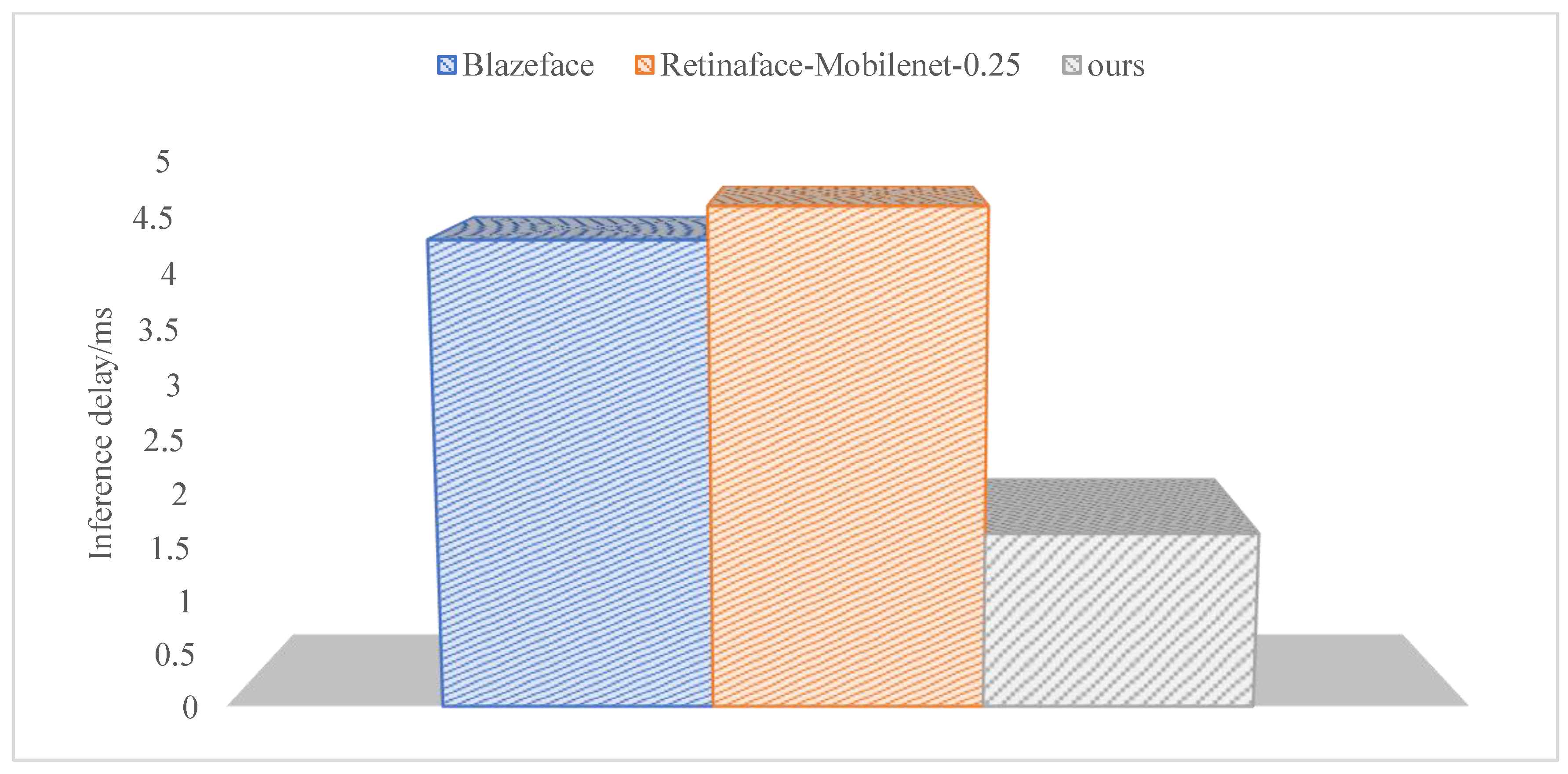
4.5. Co-Inference Acceleration Effect

In the experiment, NVIDIA JETSON NANO was used as an edge device with limited computing resources, and a PC was used as a server. The detailed configurations of NANO and PC are shown in Table 1. The traditional inference method is cloud-only, and NANO-only is inference directly on the edge device. In Figure 6, we show the impact of our first acceleration strategy under traditional reasoning which directly sends the picture to the cloud for processing. The transmission delay is an important factor affecting the end-to-end delay. In the experiment, the transmission delay accounts for more than 70% of the end-to-end delay, and in the case of worse network conditions, the proportion of transmission delay is larger. Among them, the test image resolution is 638 × 500.

This paper first considers the time when the reduced model runs directly on the NANO as the target latency, and changes the bandwidth from 50 kbps to 3500 kbps. Among them, the inference model performed on the NANO side and the PC side is performed on the CPU, which represents a resource-constrained situation. On the one hand, in the case of a poor network, this algorithm performs all tasks at the edge (NANO), that is, it performs the first step of acceleration. On the other hand, in the case of a good network, this algorithm will execute the segmentation strategy and perform the second step of acceleration to further reduce the end-to-end inference delay. In the case of better network bandwidth, the advantages of cooperative reasoning will be more obvious, as shown in Figure 7. Regardless of the circumstances, the algorithm can achieve significant advantages by accelerating the first and second steps. Compared with cloud-only, the latency of co-inference is only 26.5% of cloud-only (original model) with a bandwidth of 500 kbps, and as the network bandwidth decreases, this ratio will be smaller.

5. Summary and Future Work

Based on the CenterNet center point regression model, this paper uses a two-step acceleration strategy, which greatly reduces the computational load and inference delay of the model within a certain loss of accuracy. The algorithm prototype is implemented in the actual hardware and compared with other advanced algorithms; good results were achieved. However, in the model pruning stage, the model compression rate is fine-tuned through experience, not the global optimal solution. In future research, an automatic compression strategy can be considered, combining a variety of model compression methods to maximize the model compression rate, and in the collaborative reasoning stage, joint reasoning will be considered on multiple edge terminals and multiple servers to achieve the purpose of model parallelization reasoning.

Although we only conducted experiments on limited hardware resources, this method is general and can be deployed on other hardware resources, such as Raspberry Pi or Tx2. In addition, we worked under the paradigm of edge–cloud collaboration, which can perform efficient reasoning under limited hardware resources. Cloud security is also another area worthy of research, and face data involve the privacy of users. We can handle this problem well under the paradigm of edge–cloud collaboration, because there is no need to upload the complete face data directly to the cloud, only the intermediate data processed by the model. In the future, we will continue to make efforts in the field of cloud security.

References

1. Xu, T.; Du, D.K.; He, Z.; Liu, J. Pyramidbox: A context-assisted single shot face detector. In Proceedings of the European Conference on Computer Vision (ECCV), Munich, Germany, 8–14 September 2018; pp. 797–813. [Google Scholar]
2. Zhu, Y.; Cai, H.; Zhang, S.; Wang, C.; Xiong, Y. Tinaface: Strong but simple baseline for face detection. arXiv 2020, arXiv:2011.13183. [Google Scholar]
3. Chi, C.; Zhang, S.; Xing, J.; Lei, Z.; Li, S.Z.; Zou, X. Selective refinement network for high performance face detection. In Proceedings of the AAAI Conference on Artificial Intelligence, Honolulu, HI, USA, 27 January–1 February 2019; Volume 33, pp. 8231–8238. [Google Scholar]
4. Deng, H.; Feng, Z.; Qian, G.; Lv, X.; Li, H.; Li, G. MFCosface: A Masked-Face Recognition Algorithm Based on Large Margin Cosine Loss. Appl. Sci. 2021, 11, 7310. [Google Scholar] [CrossRef]
5. Gupta, K.D.; Ahsan, M.; Andrei, S.; Alam, K.M.R. A robust approach of facial orientation recognition from facial features. BRAIN Broad Res. Artif. Intell. Neurosci. 2017, 8, 5–12. [Google Scholar]
6. Zhuang, L.; Li, J.; Shen, Z.; Gao, H.; Zhang, C. Learning Efficient Convolutional Networks through Network Slimming. In Proceedings of the 2017 IEEE International Conference on Computer Vision (ICCV), Venice, Italy, 22–29 October 2017; pp. 2755–2763. [Google Scholar]
7. He, Y.; Zhang, X.; Sun, J. Channel pruning for accelerating very deep neural networks. In Proceedings of the IEEE International Conference on Computer Vision, Venice, Italy, 22–29 October 2017; pp. 1389–1397. [Google Scholar]
8. He, Y.; Lin, J.; Liu, Z.; Wang, H.; Li, L.; Han, S. AMC: Automl for model compression and acceleration on mobile devices. In Proceedings of the European Conference on Computer Vision (ECCV), Munich, Germany, 8–14 September 2018; pp. 784–800. [Google Scholar]
9. Ding, X.; Ding, G.; Guo, Y.; Han, J. Centripetal sgd for pruning very deep convolutional networks with complicated structure. In Proceedings of the IEEE/CVF Conference on Computer Vision and Pattern Recognition (CVPR), Long Beach, CA, USA, 15–20 June 2019; pp. 4943–4953. [Google Scholar]
10. Lin, S.; Ji, R.; Yan, C.; Zhang, B.; Cao, L.; Ye, Q.; Huang, F.; Doermann, D. Towards optimal structured cnn pruning via generative adversarial learning. In Proceedings of the IEEE/CVF Conference on Computer Vision and Pattern Recognition (CVPR), Long Beach, CA, USA, 15–20 June 2019; pp. 2790–2799. [Google Scholar]
11. Song, H.; Mao, H.; Dally, W.J. Deep compression: Compressing deep neural networks with pruning, trained quantization and huffman coding. In Proceedings of the 4th International Conference on Learning Representations (ICLR), San Juan, Puerto Rico, 2–4 May 2016. [Google Scholar]
12. Kang, Y.; Hauswald, J.; Cao, G.; Rovinski, A.; Mudge, T.; Mars, J.; Tang, L. Neurosurgeon: Collaborative Intelligence between the Cloud and Mobile Edge. ACM Sigplan Not. 2017, 52, 615–629. [Google Scholar] [CrossRef] [Green Version]
13. Paul, V.; Jones, M.J. Robust real-time face detection. Int. J. Comput. Vis. 2004, 57, 137–154. [Google Scholar]
14. Charles, B.S.; Wu, J.; Sun, J.; Mullin, M.D.; Rehg, J.M. On the design of cascades of boosted ensembles for face detection. Int. J. Comput. Vis. 2008, 77, 65–86. [Google Scholar]
15. Pham, M.T.; Cham, T. Fast training and selection of haar features using statistics in boosting-based face detection. In Proceedings of the 2007 IEEE 11th International Conference on Computer Vision, Rio De Janeiro, Brazil, 14–21 October 2007; pp. 1–7. [Google Scholar]
16. Liu, Y.; Tang, X.; Wu, X.; Han, J.; Liu, J.; Ding, E. Hambox: Delving into online high-quality anchors mining for detecting outer faces. arXiv 2019, arXiv:1912.09231. [Google Scholar]
17. Li, J.; Wang, Y.; Wang, C.; Tai, Y.; Qian, J.; Yang, J.; Wang, C.; Li, J.; Huang, F. DSFD: Dual shot face detector. In Proceedings of the IEEE/CVF Conference on Computer Vision and Pattern Recognition(CVPR), Long Beach, CA, USA, 15–20 June 2019; pp. 5060–5069. [Google Scholar]
18. Duan, K.; Bai, S.; Xie, L.; Qi, H.; Huang, Q.; Tian, Q. Centernet: Keypoint triplets for object detection. In Proceedings of the IEEE/CVF International Conference on Computer vision(CVPR), Long Beach, CA, USA, 15–20 June 2019; pp. 6569–6578. [Google Scholar]
19. Zhang, S.; Zhu, X.; Lei, Z.; Shi, H.; Wang, X.; Li, S.Z. Faceboxes: A CPU real-time face detector with high accuracy. In Proceedings of the 2017 IEEE International Joint Conference on Biometrics (IJCB), Denver, CO, USA, 1–4 October 2017; pp. 1–9. [Google Scholar]
20. Veit, A.; Belongie, S. Convolutional networks with adaptive inference graphs. In Proceedings of the European Conference on Computer Vision (ECCV), Munich, Germany, 8–14 September 2018; pp. 3–18. [Google Scholar]
21. Zeng, L.; Li, E.; Zhou, Z.; Chen, X. Boomerang: On-demand cooperative deep neural network inference for edge intelligence on the industrial Internet of Things. IEEE Netw. 2019, 33, 96–103. [Google Scholar] [CrossRef]
22. Teerapittayanon, S.; McDanel, B.; Kung, H.S. Distributed deep neural networks over the cloud, the edge and end devices. In Proceedings of the 2017 IEEE 37th International Conference on Distributed Computing Systems (ICDCS), Atlanta, GA, USA, 5–8 June 2017; pp. 328–339. [Google Scholar]
23. Shao, J.; Zhang, H.; Mao, Y.; Zhang, J. Branchy-GNN: A device-edge co-inference framework for efficient point cloud processing. In Proceedings of the ICASSP 2021–2021 IEEE International Conference on Acoustics, Speech and Signal Processing (ICASSP), Toronto, ON, Canada, 6–11 June 2021; pp. 8488–8492. [Google Scholar]
24. Jiang, N.; Xiong, Z.; Tian, H.; Zhao, X.; Du, X.; Zhao, C.; Wang, J. PruneFaceDet: Pruning lightweight face detection network by sparsity training. Cogn. Comput. Syst. 2022. early view. [Google Scholar] [CrossRef]
25. Zhao, X.; Liang, X.; Zhao, C.; Tang, M.; Wang, J. Real-time multi-scale face detector on embedded devices. Sensors 2019, 19, 2158. [Google Scholar] [CrossRef] [PubMed] [Green Version]
26. Zhu, J.; TPark, a.; Isola, P.; Efros, A.A. Unpaired image-to-image translation using cycle-consistent adversarial networks. In Proceedings of the IEEE International Conference on Computer Vision, Venice, Italy, 22–29 October 2017; pp. 2223–2232. [Google Scholar]
27. Jaderberg, M.; Simonyan, K.; Zisserman, A. Spatial transformer networks. In Proceedings of the Advances in Neural Information Processing Systems, Montreal, QC, Canada, 7–12 December 2015; Volume 28. [Google Scholar]
28. Li, E.; Zhou, Z.; Chen, X. Edge intelligence: On-demand deep learning model co-inference with device-edge synergy. In Proceedings of the 2018 Workshop on Mobile Edge Communications, Budapest, Hungary, 20 August 2018; pp. 31–36. [Google Scholar]
29. Tolias, G.; Sicre, R.; Jégou, H. Particular object retrieval with integral max-pooling of CNN activations. arXiv 2015, arXiv:1511.05879. [Google Scholar]
30. Vanholder, H. Efficient inference with tensorrt. GPU Technol. Conf. 2016, 1, 2. [Google Scholar]
31. Boqueo, G.G.; Daya, L.I.O.; Eugenio, M.E.S.; Lumagas, A.G.; Guzman, F.E.D. Extensive assessment of various network interruption tools. In Proceedings of the 2019 IEEE 4th International Conference on Computer and Communication Systems (ICCCS), Singapore, 23–25 February 2019; pp. 463–467. [Google Scholar]
32. Paszke, A.; Gross, S.; Massa, F.; Lerer, A.; Bradbury, J.; Chanan, G.; Killeen, T.; Lin, Z.; Gimelshein, N.; Antiga, L.; et al. Pytorch: An imperative style, high-performance deep learning library. In Proceedings of the Advances in Neural Information Processing Systems, Vancouver, BC, Canada, 8–14 December 2019; Volume 32. [Google Scholar]
33. Zhang, S.; Zhu, X.; Lei, Z.; Shi, H.; Wang, X.; Li, S.Z. S3fd: Single shot scale-invariant face detector. In Proceedings of the IEEE International Conference on Computer Vision, Venice, Italy, 22–29 October 2017; pp. 192–201. [Google Scholar]
34. Najibi, M.; Samangouei, P.; Chellappa, R.; Davis, L.S. Ssh: Single stage headless face detector. In Proceedings of the IEEE International Conference on Computer Vision, Venice, Italy, 22–29 October 2017; pp. 4875–4884. [Google Scholar]
35. Abdelatti, M.; Hendawi, A.; Sodhi, M. Optimizing a GPU-accelerated genetic algorithm for the vehicle routing problem. In Proceedings of the Genetic and Evolutionary Computation Conference Companion, Lille, France, 10–14 July 2021; pp. 117–118. [Google Scholar]
36. Bazarevsky, V.; Kartynnik, Y.; Vakunov, A.; Raveendran, K.; Grundmann, M. Blazeface: Sub-millisecond neural face detection on mobile gpus. arXiv 2019, arXiv:1907.05047. [Google Scholar]
37. Deng, J.; Guo, J.; Ververas, E.; Kotsia, I.; Zafeiriou, S. Retinaface: Single-shot multi-level face localisation in the wild. In Proceedings of the IEEE/CVF Conference on Computer Vision and Pattern Recognition (CVPR), Seattle, WA, USA, 13–19 June 2020; pp. 5203–5212. [Google Scholar]
Figure 1. Overall framework of the algorithm.
Applsci 12 08424 g001
Figure 2. Calculations of different layers of CenterNet-resnet18.
Applsci 12 08424 g002
Figure 3. Output n data size of different layers of CenterNet-resnet18.
Applsci 12 08424 g003
Figure 4. L 1 weight pruning flowchart.
Applsci 12 08424 g004
Figure 5. Comparison with advanced face detection models.
Applsci 12 08424 g005
Figure 6. Inference latency under cloud-only.
Applsci 12 08424 g006
Figure 7. The inference delay of the model under different bandwidths.
Applsci 12 08424 g007