
Research on the Analytical Conversion Method of Q-s Curves for Self-Balanced Test Piles in Layered Soils

Abstract
:1. Introduction
2. Analytical Conversion’s Theoretical Basis of Self-Balanced Test Pile Q-s Curve
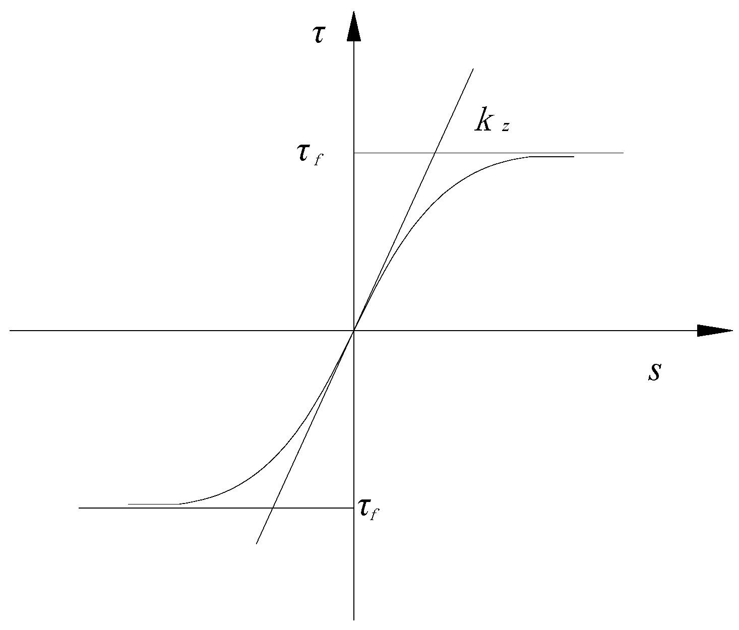
2.1. Calculation of Additional Settlement of Lower Pile Toe
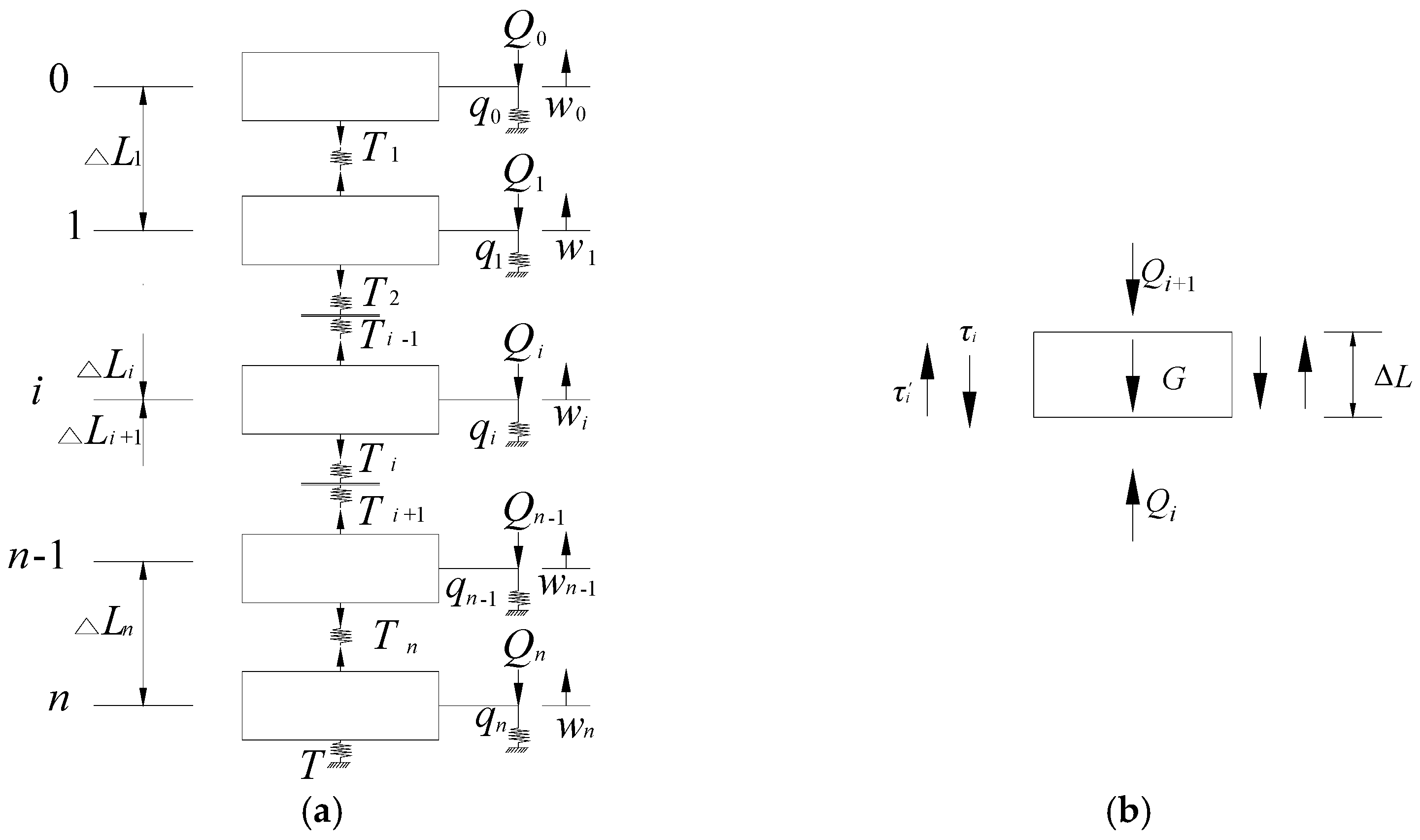
2.2. Self-Balanced Upper and Lower Piles’ Calculation Process
2.2.1. Internal Force Calculation of Self-Balanced Upper Pile
2.2.2. Self-Balanced Lower Pile Internal Force Calculation
3. Conversion Method
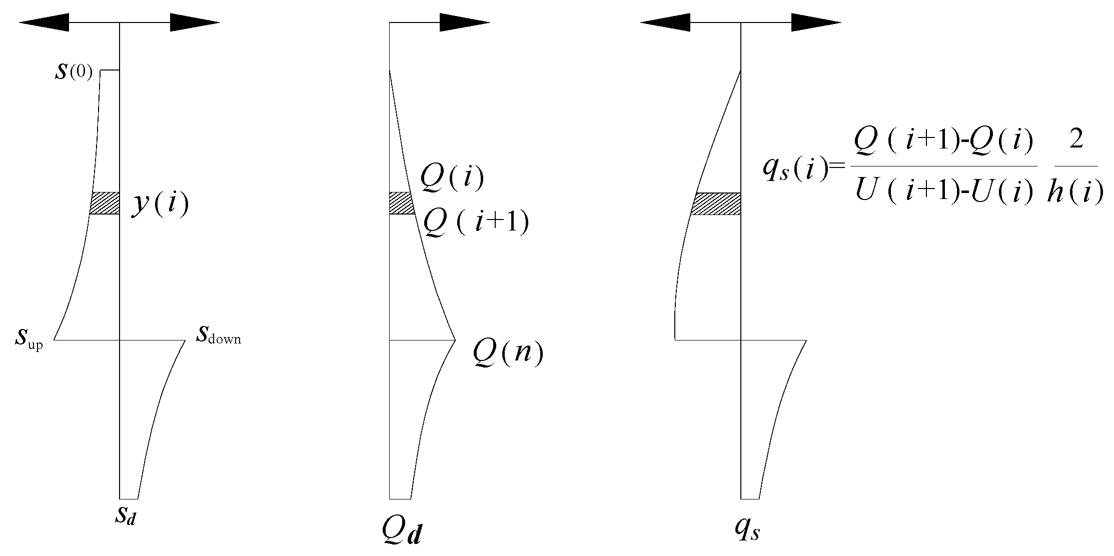
3.1. The Principle of Equivalent Conversion Equation
3.2. Conversion to Traditional Static Pressure Test Pile
4. Model Test Verification
4.1. Test Scheme
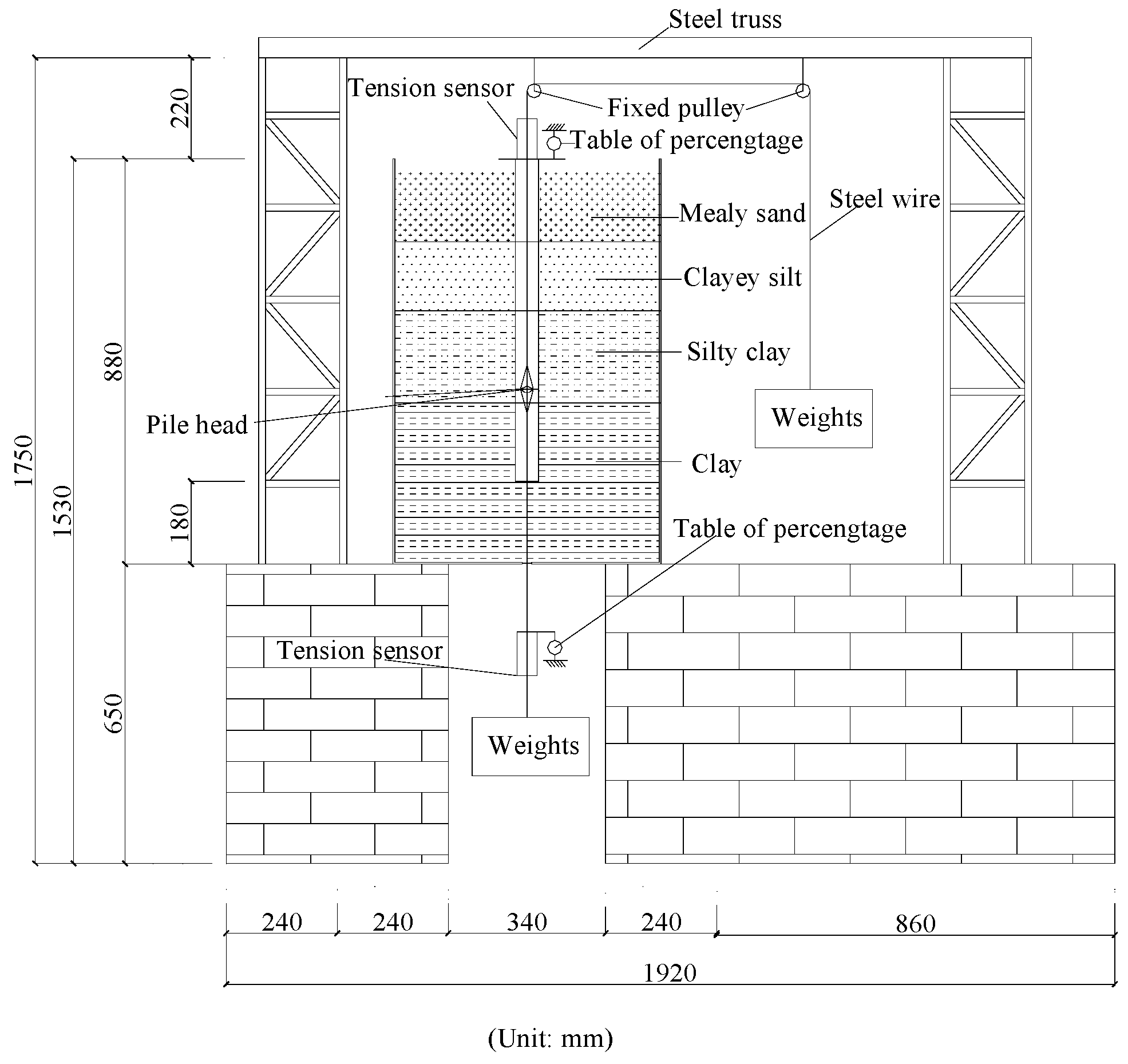
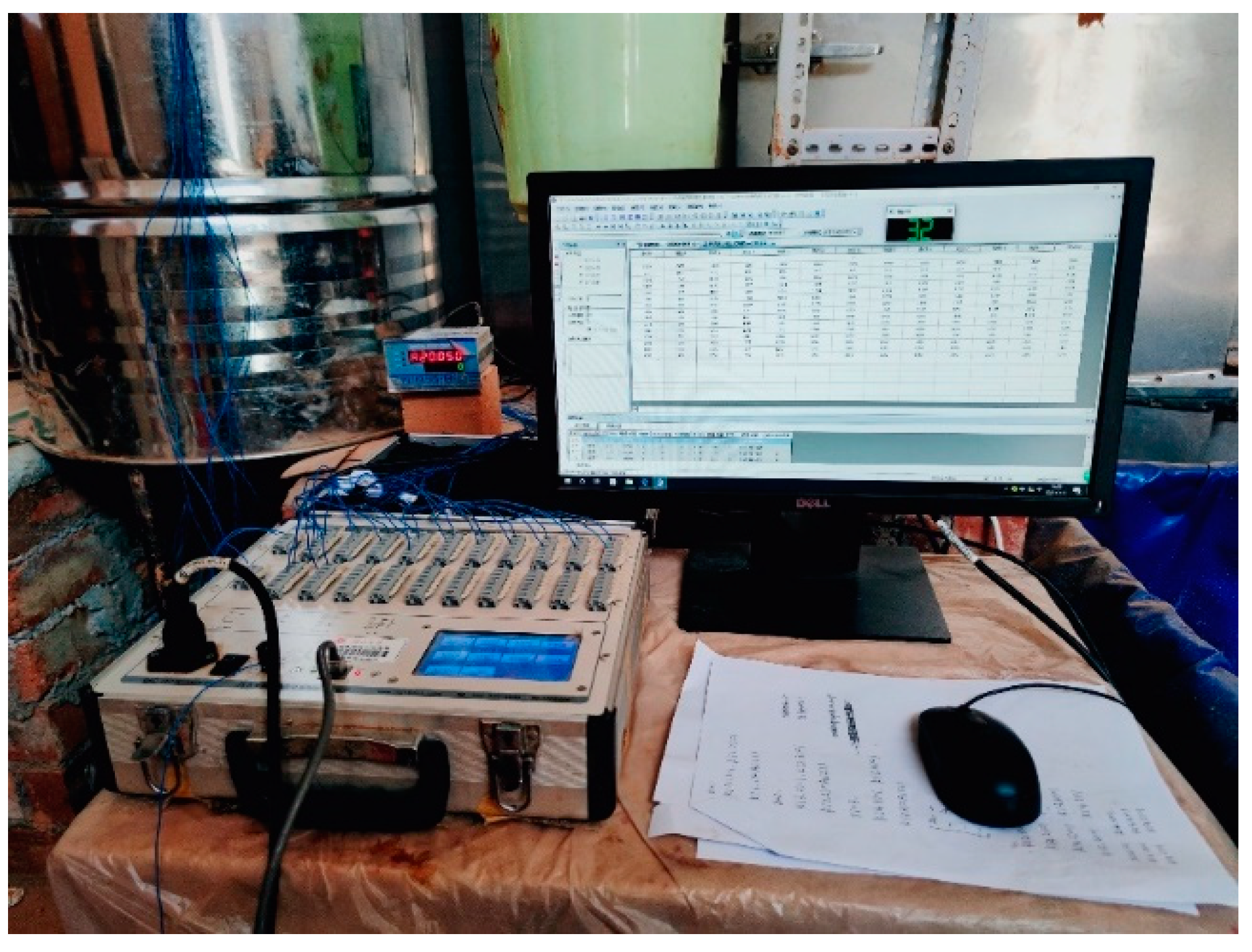
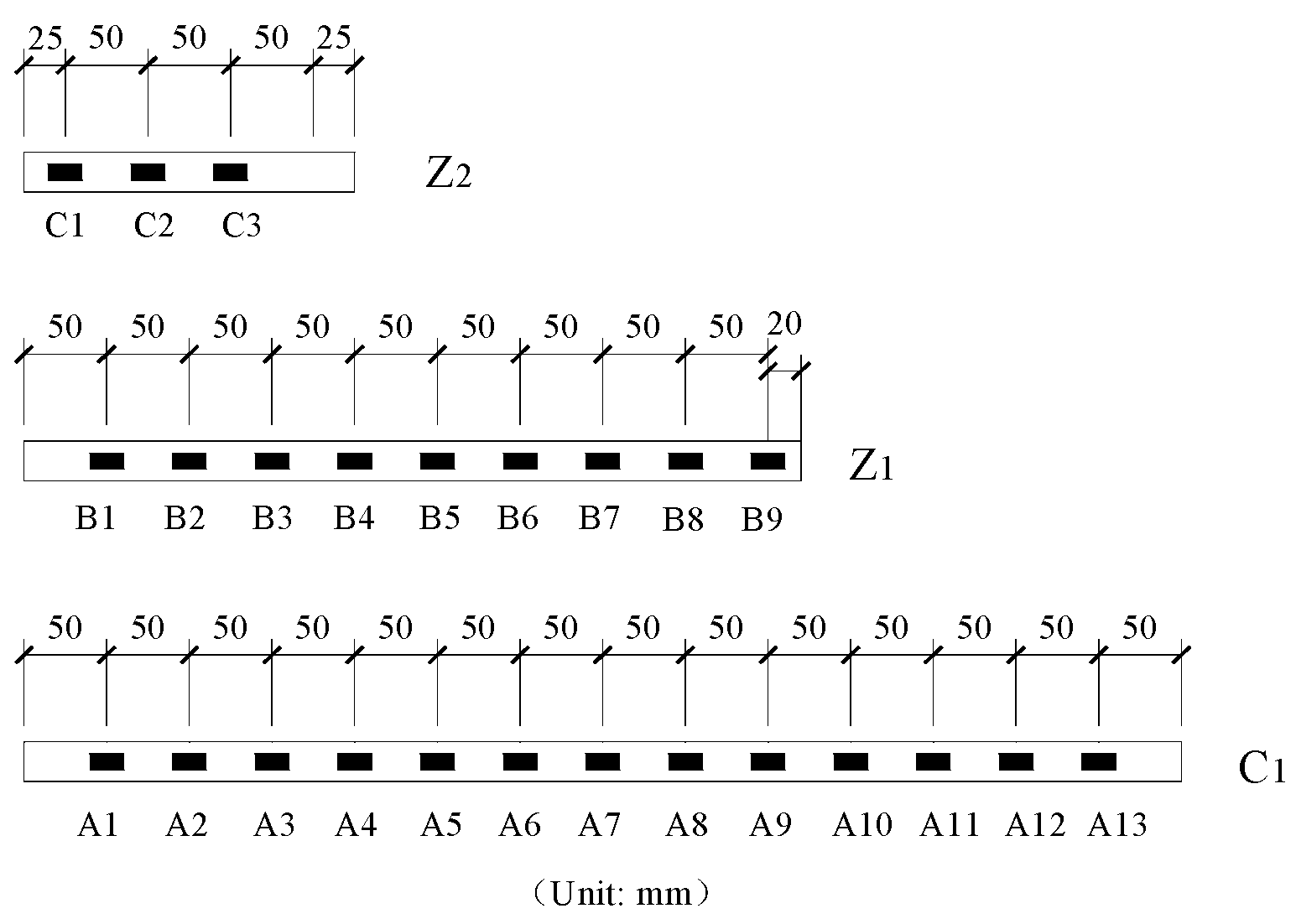
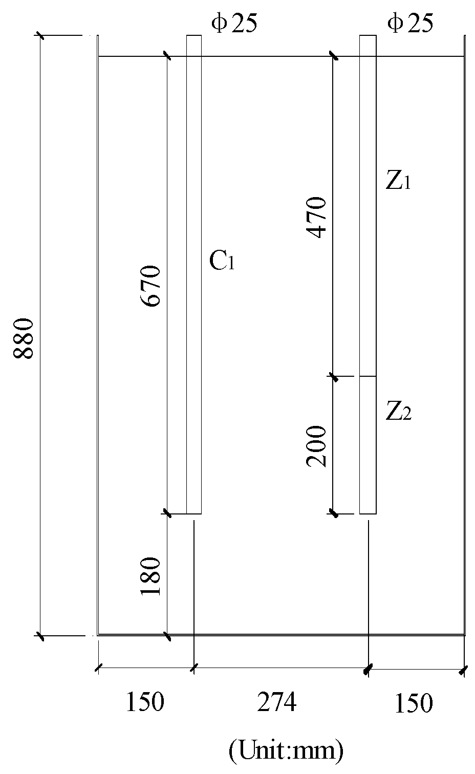
4.1.1. Test Device
4.1.2. Model Pile
4.1.3. Test Soil
4.2. Test Contents
4.3. Experiment Results and Analyses
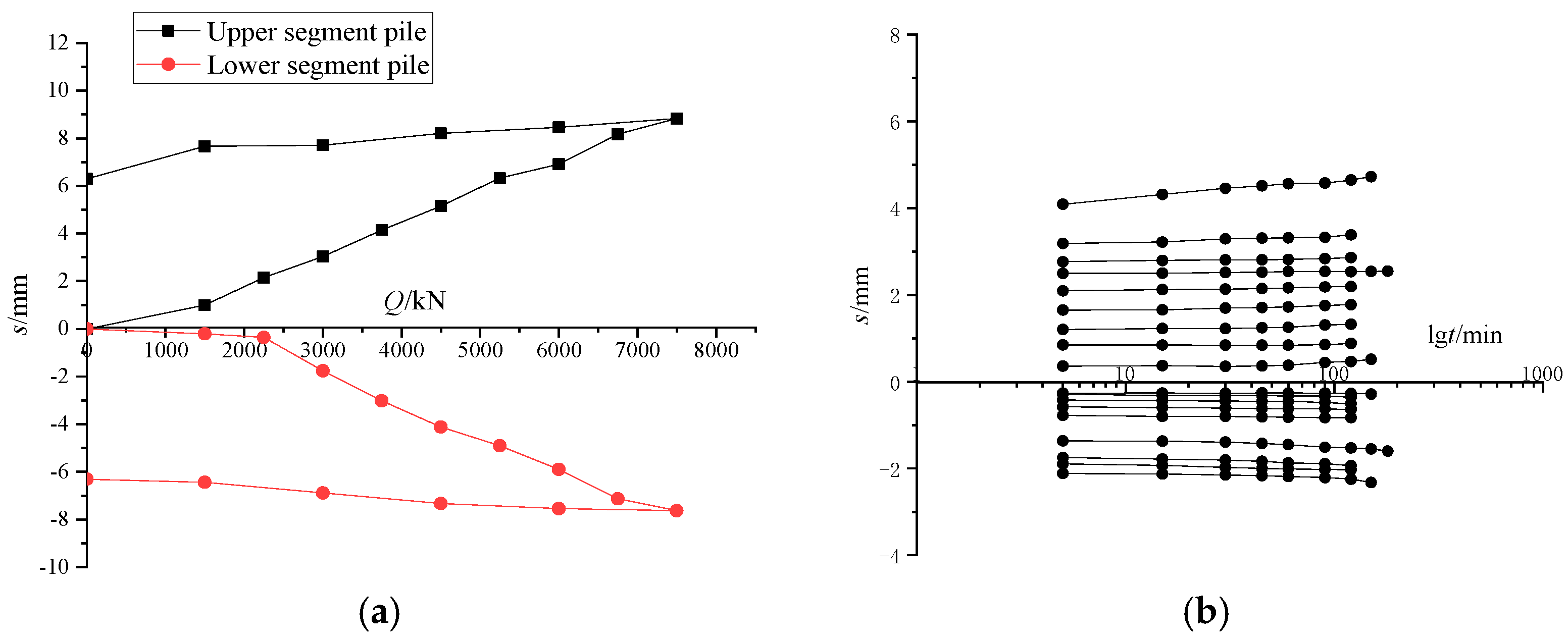
4.3.1. Experiment Results
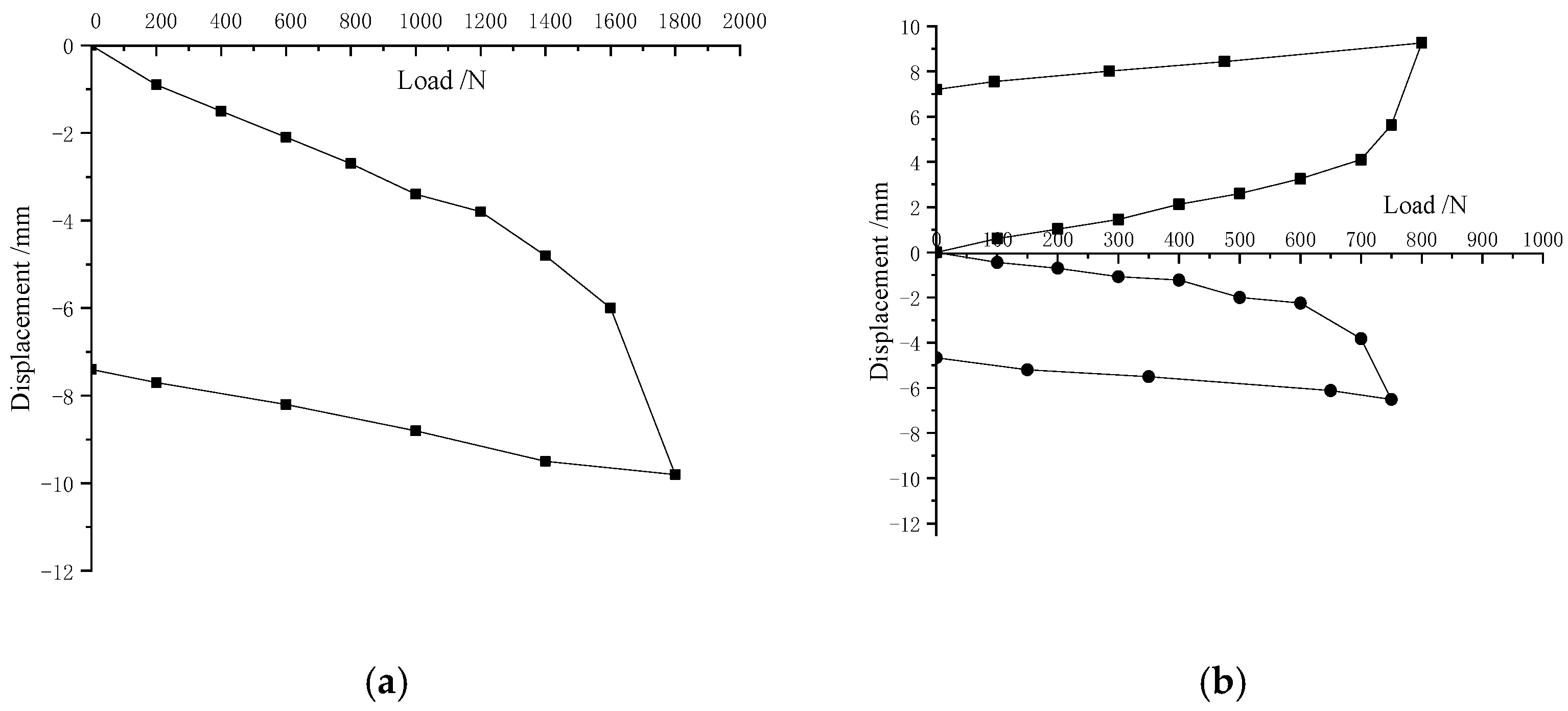
- (1)
- Loading and displacement of test piles
- (2)
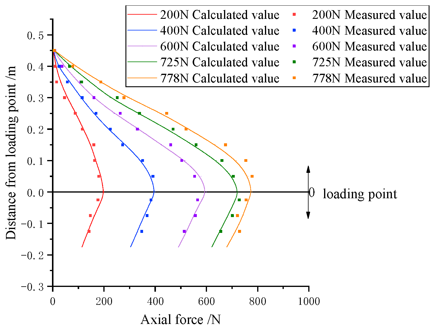
- The axial analysis of pile
- (3)
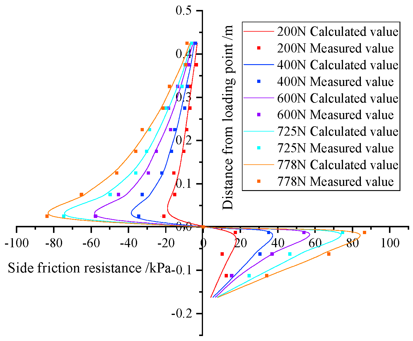
- Distribution of side friction resistance
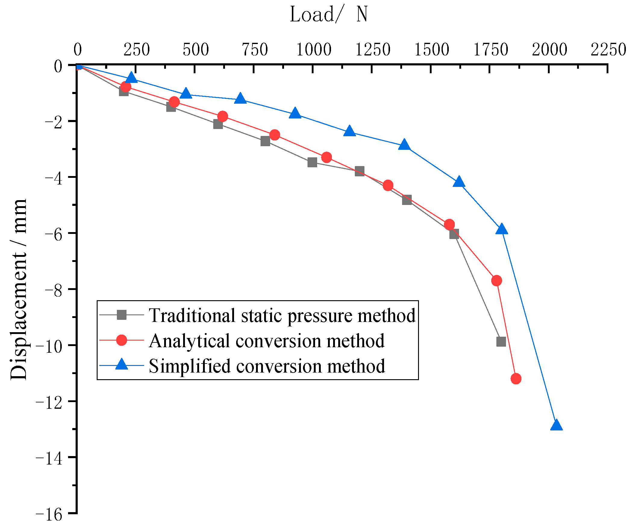
4.3.2. Equivalent Conversion Results
5. Engineering Applications
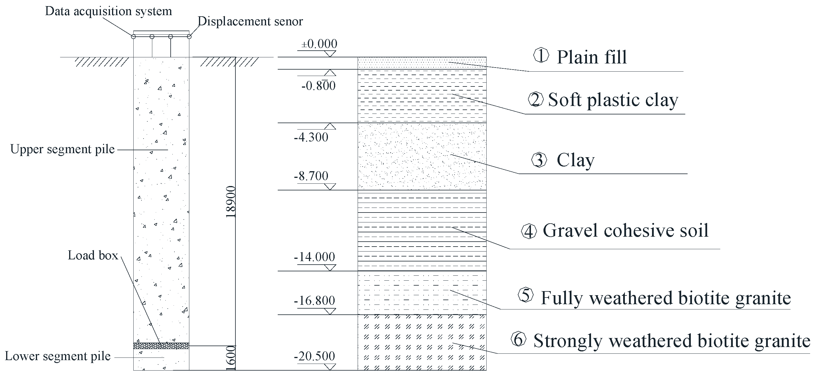
5.1. Engineering Situation
5.2. Test Result
5.3. Internal Force Analysis
5.4. Equivalent Conversion Results
6. Conclusions
Author Contributions
Funding
Institutional Review Board Statement
Informed Consent Statement
Data Availability Statement
Conflicts of Interest
References
- Poulos, H.G.; Davis, E.H. Pile Foundation Analysis and Design; John Wiley and Sons: New York, NY, USA, 1980; Available online: https://drive.google.com/file/d/0BxlQHeKi4f-6a0dBR3MzRmxUVDY0OW1tRzRMOTdoQQ/view (accessed on 3 June 2022).
- SP RK 5.01-102-2013; Foundations of Buildings and Structures. KAZGOR: Almaty, Kazakhstan, 2013.
- Askarova, N.A.; Musabayev, T.T. Comparative analysis of design and calculation of pile foundations between Eurocode 7 and national building norms of the Republic of Kazakhstan. Eur. Res. Innov. Sci. Educ. Technol. 2018, 40, 14–18. [Google Scholar] [CrossRef]
- Zhang, Z.M.; Zhang, Q.Q.; Zhang, G.X.; Shi, M.F. Large tonnage tests on super-long piles in soft soil area. Chin. J. Geot. Eng. 2011, 33, 535. [Google Scholar]
- Zhang, Z.M.; Xia, T.D.; Chen, Z.L. Experimental study on the bearing behaviors of overlength piles under heavy load. Chin. J. Rock Mech. Eng. 2005, 24, 2397–2402. [Google Scholar] [CrossRef]
- Kostina, O.V.; Bochkareva, T.M. Investigation of operation of newly designed anchor pile. J. Phys. Conf. Ser. 2021, 1928, 012060. [Google Scholar] [CrossRef]
- Shi, J.F.; Wen, D.F.; Hong, X.C.; Hong, X.L.; Yan, L.X.; Shao, F.L.; Jin, L. Field tests of micro screw anchor piles under different loading conditions at three soil sites. Bull. Eng. Geol. Environ. 2020, 80, 127–144. [Google Scholar] [CrossRef]
- Dai, Y.X.; Pan, M.G. The capacities of prefab piles on soft soil foundation determinated by pile dynamic analyzer (PDA). Chin. J. Rock Mech. Eng. 1999, 18, 104–108. [Google Scholar] [CrossRef]
- Cheng, P.F.; Ji, C.; Cui, Z.G. Static and dynamic contrast test for bearing capacity of refrozen bridge pile foundation in patchy permafrost regions. Chin. J. Rock Mech. Eng. 2015, 34, 2845–2853. [Google Scholar]
- Caio, G.N.; Henrique, S.B.; Heraldo, L.G. Probabilistic Analysis of Bored Pile Foundations in the Design Phase: An Application Example. Geotech. Geol. Eng. 2022, 40, 335–353. [Google Scholar] [CrossRef]
- Lu, S.L.; Zhang, J.; Zhou, S.R.; Xu, A.C. Reliability prediction of the axial ultimate bearing capacity of piles: A hierarchical Bayesian method. Adv. Mech. Eng. 2018, 10, 1687814018811054. [Google Scholar] [CrossRef]
- Fu, Q.; Li, X.; Meng, Z.L.; Liu, Y.N.; Cai, X.J.; Fu, H.W.; Zhang, X.P. Reliability Assessment on Pile Foundation Bearing Capacity Based on the First Four Moments in High-Order Moment Method. Shock. Vib. 2021, 2021, 2082021. [Google Scholar] [CrossRef]
- Du, Z.D.; Xu, S. Bearing Capacity Design of Ram-Compacted Bearing Base Piling Foundations by Simple Numerical Cavity Expansion Approach. Int. J. Geomech. 2022, 22, 04021284. [Google Scholar] [CrossRef]
- Wang, L.; Zheng, G.; Ou, R.N. Finite element analysis of effect of soil displacement on bearing capacity of single friction pile. J. Cent. South Univ. 2014, 21, 2051–2058. [Google Scholar] [CrossRef]
- Graine, N.; Hjiaj, M.; Krabbenhoft, K. 3D failure envelope of a rigid pile embedded in a cohesive soil using finite element limit analysis. Int. J. Numer. Anal. Methods Geomech. 2021, 45, 265–290. [Google Scholar] [CrossRef]
- Zhu, J.M.; Yin, K.C.; Gong, W.M. Discussion about several issues of bi-directional load testing in Chinese, American and European standards. Rock Soil Mech. 2020, 41, 3491–3499. [Google Scholar]
- Zhang, G.B.; Ji, T.G.; Li, Z.B. Comparison of load test results between self-balanced method and static pressure method. Chin. J. Geotech. Eng. 2011, 33, 471–474. Available online: https://www.engineeringvillage.com/search/doc/abstract.url?&pageType=quickSearch&usageZone=resultslist&usageOrigin=searchr-sults&searchtype=Quick&SEARCHID=3e603980f84c4db181cdca9f267fe5fd&DOCINDEX=1&ignore_docid=cpx_535b581340fa5cad6M55502061377553&database=1&format=quickSearchAbstractFormat&tagscope=&displayPagination=yes (accessed on 5 June 2022).
- Osterberg, J. New device for load testing driven piles and drilled shafts separates friction and end bearing. Piling Deep. Found. 1989, 1, 421–427. Available online: https://sc.panda321.com/extdomains/books.google.com/books?hl=zh-CN&lr=&id=4SgPxgQh2SwC&oi=fnd&pg=PA421&dq=+New+device+for+load+testing+driven+piles+and+drilled+shafts+separates+friction+and+end+bearing&ots=Ja7VWtW_Wa&sig=x8t581-mhEMCp5BuvulsZaaQEM4#v=onepage&q=New%20device%20for%20load%20testing%20driven%20piles%20and%20drilled%20shafts%20separates%20friction%20and%20end%20bearing&f=false (accessed on 5 June 2022).
- Xing, H.; Wu, J.; Luo, Y. Field tests of large-diameter rock-socketed bored piles based on the Self-balanced method and their resulting load bearing characteristics. Eur. J. Environ. Civ. Eng. 2019, 23, 1535–1549. [Google Scholar] [CrossRef]
- Dai, Z.R.; Huang, Z.H.; Li, H.; Yin, X.D. The application study of self-balanced test method for bearing capacity of foundation piles. Adv. Mater. Res. 2011, 243–249, 2395–2400. [Google Scholar] [CrossRef]
- ASTM D8169/D81 69M-18; Standard Test Methods for Deep Foundations under Bi-Directional Static Axial Compressive Load. ASTM: West Conshohocken, PA, USA, 2018.
- ISO 22477-1:2018; Geotechnical Investigation and Testing-Testing of Geotechnical Structures—Part 1: Test of Piles: Static Compression Load Testing. BSI: London, UK, 2018.
- JT/T738—2009; Static Loading Test of Foundation Pile Self Balance Method. Communications Press: Beijing, China, 2009. (In Chinese)
- JTG3363-2019; Specification for Design of Highway Bridges and Culverts. Communications Press: Beijing, China, 2019. (In Chinese)
- Seol, H.; Jeong, S.; Kim, Y. Load transfer analysis of rock-socketed drilled shafts by coupled soil resistance. Comput. Geotech. 2009, 36, 446–453. [Google Scholar] [CrossRef]
- Mindlin, R.D. Force at a point in the interior of a semi-infinite solid. Physics 1936, 7, 195–202. [Google Scholar] [CrossRef]
- Kim, S.R.; Chung, S.G. Equivalent head-down load vs. Movement relationships evaluated from bi-directional pile load tests. Ksce J. Civ. Eng. 2012, 16, 1170–1177. [Google Scholar] [CrossRef]
- Seol, H.; Jeong, S.; Kim, Y. Load–settlement behavior of rock-socketed drilled shafts using Osterberg-Cell tests. Comput. Geotech. 2009, 36, 1134–1141. [Google Scholar] [CrossRef]
- Niazi, F.S.; MaynePaul, W. Axial pile response of bidirectional O-cell loading from modified analytical elastic solution and downhole shear wave velocity. NRC Res. Press Can. Geotech. J. 2014, 51, 1284–1302. [Google Scholar] [CrossRef]
- Lee, J.S.; Park, Y.H. Equivalent pile load–head settlement curve using a bi-directional pile load test. Comput. Geotech. 2008, 35, 124–133. [Google Scholar] [CrossRef]
- Mission, J.L.; Kim, H.J. Design charts for elastic pile shortening in the equivalent top–down load–settlement curve from a bidirectional load test. Comput. Geotech. 2011, 38, 167–177. [Google Scholar] [CrossRef]
- Southeast University. JGJ/T. 403-2017; Technical Specification for Static Loading Test of Self-Balanced Method of Building Foundation Piles. China Architecture and Building Press: Beijing, China, 2017.
- Ou, X.D.; Bai, L.; Jiang, J.; Lyu, Z.F.; Qin, J.X. Research on analytical conversion method of self-balanced test pile results. Eur. J. Environ. Civ. Eng. 2021, 1–17. [Google Scholar] [CrossRef]
- Wang, L.J.; Zhao, Q.H.; Mao, J.Q.; Wu, J.J.; Guo, F.S. Bearing capacity and simplified calculation approach for large-diameter plain-concrete piles. Arab. J. Geosci. 2021, 14, 1480. [Google Scholar] [CrossRef]
- Lu, L.H.; Liu, A.H.; Luan, X.B. The Simplified Conversion Method for the O-Cell Load Testing Curve. Appl. Mech. Mater. 2013, 438–439, 1278–1281. [Google Scholar] [CrossRef]
- Muszyński, Z.; Rybak, J.; Kaczor, P. Accuracy assessment of semi-automatic measuring techniques applied to displacement control in self-balanced pile capacity testing appliance. Sensors 2018, 18, 4067. [Google Scholar] [CrossRef]
- Nie, R.S.; Leng, W.M.; Wei, W. Equivalent conversion method for self-balanced tests. Chin. J. Geotech. Eng. 2011, 33, 188–191. Available online: https://www.engineeringvillage.com/search/doc/abstract.url?&pageType=quickSearch&usageZone=resultslist&usageOrigin=searchresults&searchtype=Quick&SEARCHID=d0ede927acc347c6b192397994ef7d52&DOCINDEX=1&ignore_docid=cpx_535b581340fa5cad6M55872061377553&database=1&format=quickSearchAbstractFormat&tagscope=&displayPagination=yes (accessed on 5 June 2022).
- Jiang, J.; Wang, S.W.; Ou, X.D. Torsional nonlinear analysis of single pile in expansive Soil foundation. Eng. Mech. 2020, 37, 219–227. [Google Scholar] [CrossRef]
- Ai, Z.Y.; Yue, Z.Q. Elastic analysis of axially loaded single pile in multilayered soils. Int. J. Eng. Sci. 2008, 47, 1079–1088. [Google Scholar] [CrossRef]
- Kraft, L.M.; Ray, R.P.; Kagawa, T. Theoretical t-z curves. J. Geotech. Eng. Div. ASCE 1981, 107, 1543–1561. [Google Scholar] [CrossRef]
- Hou, K.W.; Jiang, J.; Wang, S.W.; Ou, X.D. Physical Model Test and Theoretical Study on the Bearing Behavior of Pile in Expansive Soil Subjected to Water Infiltration. Int. J. Geomech. 2021, 21, 06021014. [Google Scholar] [CrossRef]
- Huang, M.S.; Jiu, Y.Z.; Jiang, J.; Li, B. Nonlinear analysis of flexible piled raft foundations subjected to vertical loads in layered soils. Soils Found. 2017, 57, 632–644. [Google Scholar] [CrossRef]
- Randolph, M.F.; Wroth, C.P. Analysis of deformation of vertically loaded piles. J. Geotech. Eng. Div. 1978, 104, 1465–1488. [Google Scholar] [CrossRef]
- Cai, Y.; Xu, L.R.; Zhou, D.Q.; Deng, C.; Feng, C.X. Model test research on method of self-balance and traditional static load. Rock Soil Mech. 2019, 40, 3011–3018. [Google Scholar] [CrossRef]
- Jiu, Y.Z.; Huang, M.S. Studies on pile bearing characteristics in saturated clay under excavation by model tests and a simplified method. Chin. J. Geotech. Eng. 2016, 38, 8. [Google Scholar] [CrossRef]
- Jiang, J.; Wang, S.W.; Ou, X.D.; Fu, C.Z. Analysis of the bearing characteristics of single pile under the T→V loading path in clay ground. Adv. Civ. Eng. 2021, 2021, 8896673. [Google Scholar] [CrossRef]


| Model | Pile Length/mm | Pile Diameter/mm2 | Mass/g | Elastic Modulus/GPa |
|---|---|---|---|---|
| The self-balanced upper segment pile Z1 | 470 | 25 | 149.7 | 69.5 |
| The self-balanced lower pile Z2 | 200 | 25 | 121.4 | 69.5 |
| The traditional static pressure pile C1 | 670 | 25 | 271.1 | 69.5 |
| Soil Layer | Type of Soil Layer | Soil Thickness/mm | Water Content | Force of Cohesion/kPa | Internal Friction Angle/° | Elastic /MPa | Poisson Ratio |
|---|---|---|---|---|---|---|---|
| ① | Mealy sand | 150 | 18 | 5.5 | 36.4 | 14 | 0.35 |
| ② | Clayey silt | 150 | 18 | 7.2 | 25 | 23 | 0.35 |
| ③ | Silty clay | 200 | 26 | 25 | 19.0 | 19.0 | 0.42 |
| ④ | Clay | 450 | 26 | 59.6 | 18.0 | 28.0 | 0.40 |
Publisher’s Note: MDPI stays neutral with regard to jurisdictional claims in published maps and institutional affiliations. |
© 2022 by the authors. Licensee MDPI, Basel, Switzerland. This article is an open access article distributed under the terms and conditions of the Creative Commons Attribution (CC BY) license (https://creativecommons.org/licenses/by/4.0/).
Share and Cite
Ou, X.; Chen, G.; Bai, L.; Jiang, J.; Zeng, Y.; Chen, H. Research on the Analytical Conversion Method of Q-s Curves for Self-Balanced Test Piles in Layered Soils. Appl. Sci. 2022, 12, 8435. https://doi.org/10.3390/app12178435
Ou X, Chen G, Bai L, Jiang J, Zeng Y, Chen H. Research on the Analytical Conversion Method of Q-s Curves for Self-Balanced Test Piles in Layered Soils. Applied Sciences. 2022; 12(17):8435. https://doi.org/10.3390/app12178435
Chicago/Turabian StyleOu, Xiaoduo, Guangyuan Chen, Lu Bai, Jie Jiang, Yuchu Zeng, and Hailiang Chen. 2022. "Research on the Analytical Conversion Method of Q-s Curves for Self-Balanced Test Piles in Layered Soils" Applied Sciences 12, no. 17: 8435. https://doi.org/10.3390/app12178435
APA StyleOu, X., Chen, G., Bai, L., Jiang, J., Zeng, Y., & Chen, H. (2022). Research on the Analytical Conversion Method of Q-s Curves for Self-Balanced Test Piles in Layered Soils. Applied Sciences, 12(17), 8435. https://doi.org/10.3390/app12178435