Target Recognition and Navigation Path Optimization Based on NAO Robot

Abstract

The NAO robot integrates sensors, vision systems, and control systems. Its monocular vision system is adopted to locate the target object in the three-dimensional space of robots. Firstly, a positioning model based on monocular vision is established according to the principle of small hole perspective. Then, the position coordinates of the target center are obtained in the image coordinate system. In the model mentioned above, the relationship between position coordinates and image coordinates is established at a certain space height. According to this relationship, the two-dimensional coordinates in the image are converted into the three-dimensional coordinates in the robot coordinate system. After getting the target location, we establish the navigation map and find the optimal path under the unknown environment. Based on the simultaneous localization and the mapping (SLAM) theory, the sonar sensor of the NAO robot is used to detect the distance between the robot and the obstacles or between the robot and the end landmark. Moreover, the sonar sensor and the camera are used to distinguish the obstacle and the landmark. After the navigation map is built, the bi-directional parallel search strategy and the simulated annealing algorithm are introduced to improve the traditional artificial bee colony algorithm, and the improved artificial bee colony algorithm is proposed to find an optimal path in the navigation map. Finally, the experimental results show that based on the built environment map, the robot can find an optimal path from the origin to the landmark on the premise of avoiding obstacles.

1. Introduction

In recent years, the technology of the fully autonomous humanoid robot has developed rapidly and become the most popular research field. Robots can be used to replace workers to finish a lot of complex work and detect harsh environments. How to make robots integrate well into human life is also a hot topic [1]. Robot-based target location and navigation path planning are the most important functions of humanoid robots. The NAO robot as a bipedal robot compared to multi-legged robots and wheeled robots has the advantage of flexibility in a low gait environment, and for some specific tasks, such as target object grasping, etc., it can perform more like a human [2]. Many research results have been on target location and navigation path optimization based on the NAO robot. For example, the camera calibration is carried out to determine the parameters which define the relationship between the reference 3D coordinate system and the camera coordinate frame. These parameters are combined with the transformation and the parameters related to the camera [3]. According to the recognized objects in the robot database, the robot’s monocular camera can realize the object recognition and avoid obstacles through some measures. In actual experiments, the Nao robot can effectively perform actions in a messy environment [4], improving the gait planning under complex working conditions to save computing resources and improving the utilization of the hardware system [5]. Aiming at the problem of navigation path optimization, researchers have proposed many methods, such as the SLAM theory for the recognition in [6] and the localization in an unknown environment or the algorithms based on the artificial intelligence for navigation in [7,8,9]. The SLAM theory is useful to help robots build maps in an unknown environment, so it was adopted in this paper. The ant colony optimization algorithm (ACO) is proposed to find the optimal path in [10,11,12,13,14]. Meanwhile, the genetic algorithm (GA) is proposed to solve the path optimization problem in [15]. Furthermore, more optimization algorithms such as the particle swarm optimization algorithm (PSO) and the neural network algorithm are also applied to solve the path optimization problem [16,17,18]. However, the disadvantage of these traditional optimization algorithms is that it is easy to fall into the local optimum, and the convergence speed is slow. The best optimization results of these traditional optimization algorithms may not be found, and they need a long time to be explored. To get more efficient and stable optimization results, the bi-directional parallel search strategy and the simulated annealing algorithm are introduced to improve the traditional artificial bee colony algorithm (ABC) in this paper. By improving the artificial bee colony algorithm (IABC), not only the optimal path can be obtained based on the built environment map, but also the convergence speed is faster than other optimization algorithms [19,20,21].

This paper mainly takes the Nao robot as the research platform to solve the problems of the robot space target localization and navigation path optimization. The main contribution of this paper is presented as follows: (1) The K-means algorithm and Q-learning algorithm are combined to make the NAO robot avoid obstacles in the process of moving. The former algorithm is used to classify the obstacle and calculate its accurate distance, and the latter algorithm is adopted to help the robot to build an environment map. (2) The improved artificial bee colony algorithm (IABC) is proposed based on the bi-directional parallel search strategy and simulated annealing algorithm after the navigation map built. The IABC algorithm is applied to find an optimal path in the navigation map and has faster convergence and better solutions compared to the traditional optimization algorithm. (3) A positioning model based on monocular vision is established according to the principle of small hole perspective. Moreover, the position coordinates of the target center are obtained in the image coordinate system. Finally, the experimental results show that based on the built environment map, the robot can find an optimal path from the origin to the landmark on the premise of avoiding the obstacles, and a faster convergence speed can be obtained with the improved artificial bee colony algorithm.

This paper is organized as follows: In Section 2, target recognition and localization are introduced. In Section 3, the navigation theory is introduced, and the navigation experiment method is designed. In Section 4, the improved artificial bee colony algorithm is used to find the optimal navigation path for mobile robots. The experiment result is given in Section 5. Finally, the conclusion is drawn in Section 6.

2. NAO Robot’s Monocular Vision Spatial Target Localization

Because the NAO robot can only work with a single camera, this paper proposed to use the monocular vision positioning technology for target positioning. First, a monocular vision positioning model is established [22]. Through the geometric calculation, the two-dimensional coordinates in the image are transformed into three-dimensional coordinates in the robot coordinate system to achieve the spatial target positioning. As a typical system of visual positioning system [23], the monocular vision system has achieved many research results on the target position positioning model. However, the height of the actual target object has been ignored in many studies. In the grasping experiment based on the Nao robot, the object should appear at a certain height, so the positioning based on the plane target cannot meet the requirements. In this paper, the position coordinates of the target center in the image coordinate system are obtained with the image recognition method, and then the monocular vision positioning model is used to establish the relationship between the positions coordinates and the image coordinates at a fixed height in space. Finally, the position coordinates of the target in the NAO robot coordinate system are obtained.

2.1. Image Preprocessing

As the basis of target recognition, image preprocessing is also the data module of subsequent image processing stages. First, the image needs to be separated and filtered through specific channels [24]. The color image formats supported by Nao robots mainly include YUV422, RGB, and HSV, among which RGB color space is the most common. It is composed of three colors: R (red), G (green), and B (blue). Other colors are composed of them in different proportions [25]. During the experimental test, it is found that in general, the red ball can be accurately separated using either RGB or HSV color spaces. However, in the case of poor light (too strong or too weak), HSV color space is more stable. Therefore, this paper adopts HSV color space as the color space of the Nao robot visual image processing.

How to separate the target from the image according to the threshold is also one of the important tasks of robot target recognition. For the color image obtained with the camera, it is difficult to separate the target with binarization according to a threshold, so it is necessary to sample and calibrate the thresholds of the three components. Under the illumination condition of the actual experimental environment, select the color area of the target in the image, count the color characteristics of each point, and get the upper and lower limit values of each component in the HSV color space [26]. The image is binarized according to the threshold, and the results are observed and adjusted in time. When the effect is ideal, the corresponding threshold is recorded as the final threshold. After the threshold is determined, the image needs to be filtered. Because Gaussian filtering can effectively suppress noise and smooth the image, this paper uses Gaussian filtering [27] to blur the local information of the image, which is conducive to the next step of Hough circle detection [28].

2.2. Target Recognition

In the image preprocessing stage, the red image areas have been marked, but these areas contain some interference, which needs to be further extracted through geometric features. Hough circle detection [29,30] is used in this paper to further extract the target and obtain its central coordinates. In the process of using the Hough circle transformation to detect the shape, each boundary pixel (x, y) of the image is extracted with the Canny detection algorithm, and then judged according to Equation (1). If the three parameters of the detection circle, namely C (x₀, y₀, r), meet Equation (1), the value of the accumulator will be increased by 1, and finally, a group of peaks will be selected, which is the required center coordinates and radius.

$${(x-x_0)}^2+{(y-y_0)}^2-r^2\le \delta$$

(1)

During the experiment, many small balls may be detected using the Hough circle transform, which may also contain some noise, so the results need to be further processed. For each red ball detected, a green circumscribed square, with the center of the red ball and 4 times the radius of the red ball as the side length, is drawn. Then, we calculate the ratio of red and green pixels in the square area. In the ideal case, the proportion of red pixels is 0.196, as shown in Equation (2), and the proportion of green pixels is 0.804. In the actual detection, there are many uncertain factors (such as circle detection error, a color change caused by uneven light, interferences, etc.), which are difficult to achieve in the ideal situation. During the experiment, we set the condition that the percentage of red and green pixels is 0.12 and 0.1, respectively.

$$(\pi r^2)/(16r^2)=0.196$$

(2)

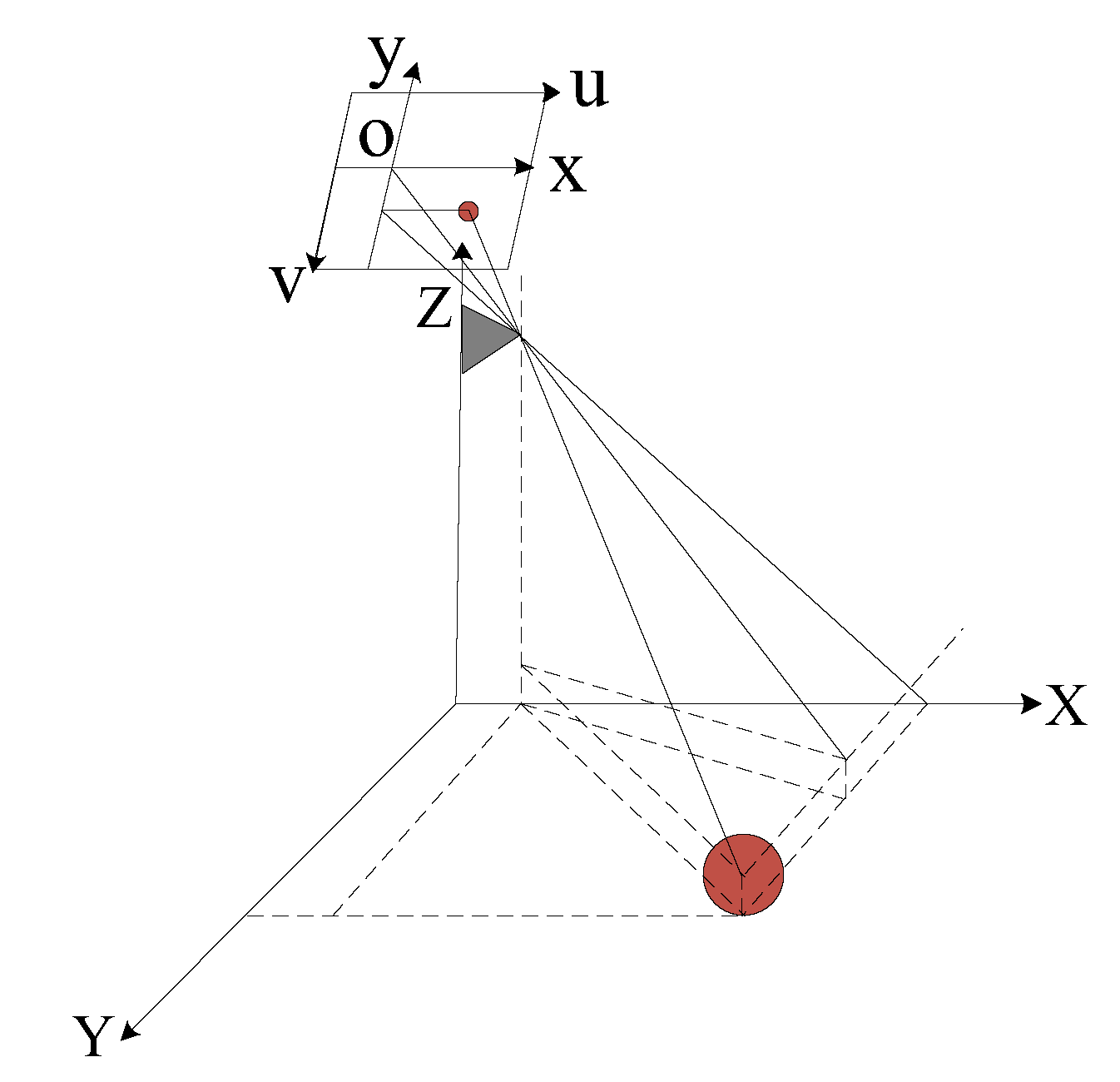
2.3. Monocular Vision Location and Ranging

The monocular vision positioning model is shown in Figure 1. According to the small hole perspective model, the position of the target in space is obtained through the transformation between the image coordinates and the actual space coordinates. When positioning the target object in robot coordinates, the height of the target should be lower than that of the camera.

The local image can be obtained by observing the monocular vision positioning model, in which (a) top view, (b) side view, and (c) image coordinate system is shown in Figure 2.

In the figure, ${\theta }_{headpitch}$ is the head pitch angle, ${\theta }_{headyaw}$ is the head deflection angle, ${\theta }_{ballpitch}$ is the vertical field angle, ${\theta }_{ballyaw}$ is the horizontal field angle, H is the camera height,$w$ is the image width, $h$ is the image height, (X₀, Y₀) is the image coordinate system coordinates, (X₁, Y₁) is the world coordinate system coordinates, $r$ is the small ball radius, ${\theta }_{c\_direction}$ is 47.64°.

After image preprocessing, (X₀, Y₀), $w$ and $h$ are the image resolution $640\times 480$ pix, ${\theta }_{c\_pitch}$ is the maximum value of the camera’s vertical field angle, ${\theta }_{c\_yaw}$ is the maximum value of the camera’s pitch angle, where H, ${\theta }_{headpitch}$, $X_{camera}$, $Y_{camera}$ are obtained through internal functions.

$${\theta }_{ballpitch}=\frac{(Y_0-240)\times {\theta }_{c\_pitch}}{480}$$

(3)

$${\theta }_{ballyaw}=\frac{(320-X_0)\times {\theta }_{c\_yaw}}{640}$$

(4)

$$d_{pitch}=\frac{\left(H-r\right)}{tan(\frac{{\theta }_{c\_direction}\times pi}{180}+{\theta }_{headpitch}+{\theta }_{ballpitch})}$$

(5)

$$d_{yaw}=\frac{d_{pitch}}{cos{\theta }_{ballyaw}}$$

(6)

$$X_1=d_{yaw}\times cos\left({\theta }_{ballyaw}+{\theta }_{headyaw}\right)+X_{camera}$$

(7)

$$Y_1=d_{yaw}\times sin\left({\theta }_{ballyaw}+{\theta }_{headyaw}\right)+Y_{camera}$$

(8)

From Equations (3)–(6), the coordinates of the small ball world coordinate system (X₁, Y₁) can be obtained. When the ball has a certain height, the NAO robot coordinate system is taken as the three-dimensional coordinate system. The height of the small ball is $h_1$, modify Equation (5).

$$d_{pitch}=\frac{\left(H-r-h_1\right)}{tan(\frac{{\theta }_{c\_direction}\times pi}{180}+{\theta }_{headpitch}+{\theta }_{ballpitch})}$$

(9)

Bring Equation (9) into Equation (6) to get the coordinates of the ball at a certain height; $h_2$ is the height from the origin to the ground under the robot coordinate system. The coordinates of the ball in the robot coordinate system are (X₁, Y₁, $r+h_1-h_2$).

There is a certain error in the spherical coordinates obtained by calculation. To eliminate the error, the error coefficient k is proposed to compensate for the actual distance, as shown in:

$$X=k\times x.$$

(10)

The error coefficient k can be solved with a quartic polynomial:

$$k=a{x}^4+b{x}^3+c{x}^2+dx+e$$

(11)

Remark 1.

Since the two cameras of the NAO robot are on the forehead and mouth (hardware structure design problem), the overlapping area scanned with the two cameras is small. Thus, the stereo vision and full vision systems cannot be used in the NAO robot. Furthermore, as a typical system of visual positioning system, the monocular vision system has achieved many research achievements on the target location model, which has good stability.

3. Navigation Theory and Navigation Map

3.1. Simultaneous Localization and Mapping Theory

The SLAM is a theoretical framework to build real-time location and graphs, which are widely used in navigation task. At present, the theory has a lot of development, such as the EKF-SLAM algorithm, the visual SLAM algorithm, and so on. The basic theory of the SLAM is that the robot avoids obstacles automatically and navigates by walking. To pinpoint the robot’s current position, the grid theory is introduced. The robot’s current position can be seen as one of the grids of the area. The robot walks from the current grid to the next grid. The procedure is shown in Figure 3.

In the theoretical framework of SLAM, there are two important concepts, the Q-learning algorithm, and the K-means algorithm, to help the robot build an environment map.

3.2. Q-Learning Algorithm

Q-learning algorithm is a method of online iterative calculation and incremental learning, which can use an autonomous agent to achieve the objective optimal action through constant learning and selection under the premise of not establishing the environmental model. With the increase of self-learning times, the value of $Q$ becomes larger and larger until convergence in the end. Therefore, updating the value of $Q$ is the key to the Q-learning algorithm. The update rule is written as Equation (12).

$$Q\left(s,a\right)=R\left(s,a\right)+\gamma \underset{\widehat{a}}{\max }Q\left(\widehat{s},\widehat{a}\right).$$

(12)

where $R\left(s,a\right)$ is the reward element, $Q\left(s,a\right)$ is the training value of action $a$ under the state $s$, $\underset{\widehat{a}}{\max }Q\left(\widehat{s},\widehat{a}\right)$ is the maximum value of all possible actions in the next state $\widehat{s}$, $\gamma \in \left(0,1\right)$ and is a learning parameter.

3.3. K-Means Algorithm

K-means algorithm [11] takes the Euclidean distance as the similarity criterion and the error sum of squares as the criterion function, which means taking the distance between the data points and the prototype as the optimized objective function and getting the adjustment criterion of the iterative operation using a method for finding the extreme value of the function.

The raw data set is $\left(x_1,x_2,\dots ,x_n\right)$, each datum $x_i$ is the dimensional vector of $d$. The purpose of clustering is to classify the raw data into $k$ class under the condition of the given classification group number $k$, namely $S=\left\{S_1,S_2,\dots ,S_k\right\}$. In the numerical model, the minimum value is adopted in Equation (13).

$$\underset{\mathrm{S}}{\arg \min }{\displaystyle \sum }_{i=1}^k{\displaystyle \sum }_{x_j\in S_i}\parallel x_j-{\mathsf{\mu }}_i{\parallel }^2$$

(13)

3.4. Navigation Map Building

The main purpose of the robot navigation path study is to update the value of $Q$ at different states and different behaviors in real-time. There are four movement directions of the robot from the current state to the next state: forward, backward, left, and right. The selection of next state depends on the value of $Q$. The movement probability P is introduced to decide next direction. The movement probability is written as Equation (14).

$$P\left(a_i|s\right)=\frac{Q\left(s,a_i\right)}{{\displaystyle \sum _j^4\left|Q\left(s,a_j\right)\right|}}$$

(14)

where $P\left(a_i|s\right)$ represents the probability of direction $a_i$ in the current state $s$. $Q\left(s,a_i\right)$ represents the $Q$ value of direction $a_i$ in the current state $s$. The direction of maximum probability is the direction of the robot to move to a new state.

Before the robot begins to execute the navigation task, the initial value of $Q$ is 0 in any behaviors in any state, the robot updates the value of $Q$ in real-time during walking according to the surrounding environment. When the robot meets obstacles, a penalty factor is added. When the robot meets the final landmark, an incentive factor is added. The scope of the obstacle is $R_1$, when the distance between the obstacle and the robot is less than $d_1$; the penalty factor $R\left(s,a\right)$ is −100, namely, $R\left(s,a\right)=-100$. The scope of the end landmark is $R_2$, when the distance between the final landmark and the robot is less than $d_2$; the incentive factor $R\left(s,a\right)$ is 100, namely, $R\left(s,a\right)=100$. Figure 4 shows this process.

The value of the penalty factor and incentive factor is written as Equation (15).

$$R\left(s,a\right)=\{\begin{array}{cc}100& r<d_1\\ 0& \left(r>d_1\right)\&\&\left(r>d_2\right)\\ -100& r<d_2\end{array}$$

(15)

where $r$ represents the distance between the robot and obstacles or between the robot and the final landmark in the current state.

In many cases, the traditional K-means algorithm can only classify specified groups which limit the popularization of the K-means algorithm. Therefore, the traditional K-means algorithm is improved in this experiment. The procedure of classifying data with the improved K-means algorithm is as follows:

(1)

Randomly choose k elements from n elements as the center of k clusters.

(2)

According to average, each object is assigned to similar clusters.

(3)

Recalculate the distance between each cluster and the shortest cluster.

(4)

If the distance of any two clusters is less than $d_0$, the two clusters are merged. The average distance of two original cluster centers is taken as the center of a new cluster. Otherwise, go to step (2) to continue.

(5)

If the result no longer changes, the algorithm is over. Otherwise, go to step (4) to continue.

The procedure of Simultaneous Localization and Mapping is as follows under the premise of avoiding obstacles:

(1)

Collect the surrounding environment with two sonar sensors.

(2)

Classify these data with the K-means clustering algorithm to detect the number of obstacles and the distance between robot and obstacle.

(3)

Make sure the value of penalty and incentive factor according to the detecting results.

(4)

The robot updates $Q$ value according to Equation (12).

(5)

The robot selects the next state according to Equation (14).

(6)

If the robot meets the end landmark, the experiment is over. Otherwise, go to (1) to continue.

4. Optimal Navigation Path for Mobile Robot

4.1. Map Environment Design for Path Planning

The step length of the NAO robot is 0.04m, and four steps are taken as a grid with the size of 0.16m. According to the preset mapping data, the obstacle map is established in MATLAB, as shown in Figure 5. The initial coordinates are (4, 5), and the end positions are (16, 16), in which there are two obstacles.

4.2. Improved ABC Algorithm for Finding the Optimal Path

After the map is built, the optimal path can be searched with an improved artificial bee colony algorithm in the map. However, the traditional ABC algorithm adopts a roulette strategy. The strategy has the disadvantage of slow convergence speed and local optimum. To find a better path, a bi-directional parallel search strategy and simulated annealing algorithm are introduced to improve the traditional artificial bee colony algorithm.

In the process of searching the optimal path, every time a bee walks a grid, the direction is random. The bee may move in the grid of obstacles, so the method of weight is introduced to decide the path length in Equation (16):

$$L={\mu }_{n}l+{\mu }_{o}l$$

(16)

where $L$ is the path length, $l$ is the path length at each step, ${\mu }_n$ is the weight factor without obstacles, ${\mu }_o$ is the weight factor with obstacles.

The basic theory of the bi-directional parallel search strategy is that the searcher $X_s$ at the beginning and the searcher $X_e$ at the end search the optimal path at the same time. If the two search paths overlap, the search path of two searchers is deemed as the best path. The bi-directional parallel strategy contains three situations:

(1)

The two search paths do not overlap as Figure 6. The search path is the shortest path.

(2)

The two searchers meet at a point as Figure 7. The search path is the common search path.

(3)

The two search paths overlap as Figure 8. The search path is the overlap path and another search path.

The simulation annealing algorithm is from the solid annealing principle. The algorithm is used in the combinatorial optimization field and adopts an iterative solution strategy. The simulation annealing algorithm makes temperature decrease from a large value at certain parameters based on the principle of temperature drop. The procedure of updating food source with the simulation annealing algorithm is as follows:

(1)

Initialize starting temperature value.

(2)

The food source is updated at each generation, the fitness of the new food source is $fitnes{s}_{new}$, and the fitness of the original food source is $fitnes{s}_{old}$, If $fitnes{s}_{new}-fitnes{s}_{old}\le 0$, nothing is done. Otherwise, calculate $\Delta fitness=fitnes{s}_{new}-fitnes{s}_{old}$.

(3)

Determine whether to replace the original food source with $P=e^{-\frac{\Delta fitness}{kT}}$, where $k$ is a parameter between 0 and 1. $T$ is the temperature value at every moment and satisfies $T\left(t\right)=kT\left(t-1\right)$, namely, the current temperature value is the temperature after the decay of the last time.

The simulation annealing algorithm will be finished if the optimization process is over. Otherwise, go to (2) to continue.

When bees search the new food source around the original food source, a bi-directional parallel search strategy is adopted. Figure 9 shows that searchers at the beginning and the end find a random position in the original path and continue searching a new path from this position. Suppose the fitness of the new food source is better than the original. In that case, a simulated annealing algorithm is introduced to decide whether the new food source will replace the original food source.

Remark 2.

The most important feature of the simulated annealing algorithm is that it can obtain more possible solutions than other algorithms when selecting the initial solution. This ensures that it does not fall into local optimality prematurely at the initial stage of the algorithm due to the tendency of the solutions. As the algorithm enters the later stage, the control parameter t decreases, and the possibility of accepting inferior solutions gradually decreases, and when t reaches the limit, the possibility of accepting inferior solutions disappears, and the probability approaches zero. In this way, after the artificial bee colony algorithm falls into the local optimum, the ability to jump out of the local optimum can be greatly improved, so that the global optimum can be obtained more effectively for the optimization problem. By using the characteristics of the simulated annealing algorithm to improve the artificial bee colony algorithm, it is possible to avoid the IABC algorithm from falling into local minima to ensure its stability.

5. Experimental Verification

5.1. Experimental Algorithm Verification

To verify the performance of the IABC algorithm, the ant colony optimization algorithm, the Chaotic genetic algorithm, and the traditional artificial bee colony algorithm are used to compare with the improved artificial bee colony algorithm.

Table 1. The parameters of the artificial bee colony algorithm.

Parameters	Value
Food sources numbers	50
Search times	2000 times
No obstacle weight factor	0.2
Obstacle weight factor	0.8
Initialize temperature value	10
Temperature attenuation coefficient	0.8

shows these parameters of the improved artificial bee colony algorithm.

The fitness curve is shown, and the convergence speeds of the ABC algorithm and the IABC algorithm can be seen in Figure 10. The optimal path obtained with the improved artificial bee colony algorithm is better than that obtained with other algorithms. After 400 times, the traditional artificial bee colony algorithm converges to a stable value. However, only after 266 times, the improved artificial bee colony algorithm converges to a stable value.

The experiment result of the steps is shown in Figure 11. From this figure, the optimal path is 16 steps with the traditional artificial bee colony algorithm, but only 13 steps can be found with the improved artificial bee colony algorithm, so the improved artificial bee colony algorithm can find the optimal path and has a faster convergence speed.

The optimized path obtained with the offline IABC algorithm is imported into the NAO robot for online experimental verification. The experimental process is as follows: the step length of the NAO robot is set to 0.04m, and the walking path of the NAO robot is set again according to Figure 11b and

Table 2. Path setting for the NAO robot.

Grid Coordinates	Actual Path Coordinates (m)	Route Setting
(4, 5)	(0.64, 0.80)	Along the upper right 45° walk 1.131 m
(9, 10)	(1.44, 1.60)	Turn right 45° and walk for 0.16 m
(10, 10)	(1.60, 1.60)	Turn left 45° and walk for 0.679 m
(13, 13)	(2.08, 2.08)	Turn right 45° and walk for 0.16 m
(14, 13)	(2.24, 2.08)	Turn left 45° and walk for 0.32 m
(16, 15)	(2.56, 2.40)	Turn left 45° and walk for 0.16 m
(16, 16)	(2.56, 2.56)	Arrive the destination target

, with the previous termination point coordinates as the starting point coordinate and the starting point coordinate as the termination point coordinate. The comparison results of the verification are shown in Figure 12.

It can be seen from Figure 12 that the optimal setting line in the path optimization simulation of the IABC algorithm does not encounter obstacles; so according to the set path, Nao will not encounter obstacles when walking on this experimental platform. When the Nao robot reaches the position with coordinates of (2.56 m, 2.56 m), it stops walking. However, due to the material problems of the bottom of the NAO’s foot and the floor, the insufficient friction between the bottom of the foot and the ground, and the accuracy of the deflection angle, Nao produces a certain offset during walking. Therefore, the actual effect of walking on the optimal path will differ from that under the ideal condition, but it is within the allowable range of error. The Nao robot can realize path optimization while avoiding obstacles.

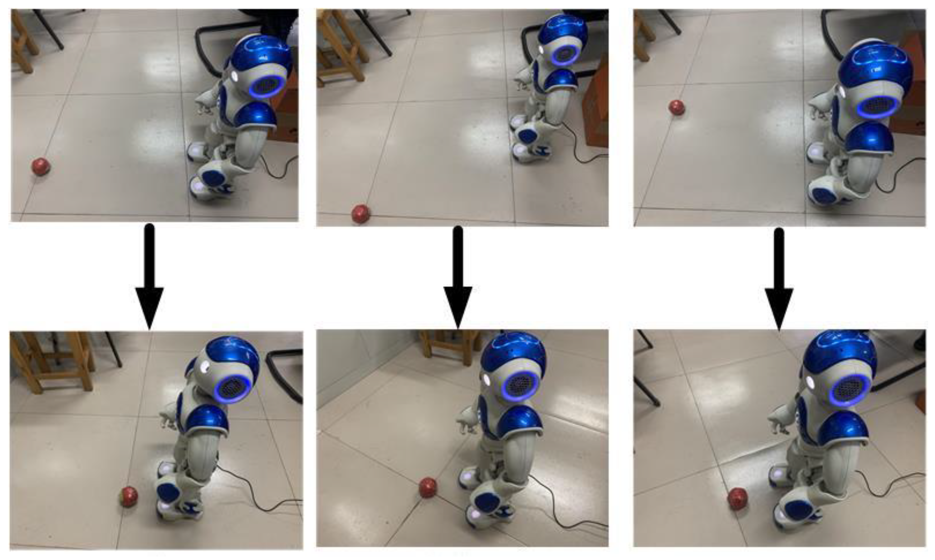
5.2. NAO Robot Experimental Validation

To verify the feasibility of the IABC algorithm on the NAO robot, the map was constructed offline, and the path was optimized, and experiments were conducted online to verify. NAO robot is a bipedal intelligent robot developed by Aldebaran Robotics, which combines many sensor devices into one, and its hardware equipment includes CPU, ultrasonic, gyroscope, infrared, and so on. The two camera sensors on the NAO robot are regarded as the main hardware facility of the vision location system, one on the forehead and one on the mouth, that can “see” things around it. The camera can take both photo images and record videos, all implemented by NAO’s vision software module. As seen in Figure 13, the NAO robot can achieve recognition of targets at different locations and reach the specified location as expected.

6. Conclusions

The NAO robot can obtain the position coordinates of the target based on the monocular vision system and then walk near the target. The experimental results show that the target position error is about 1~2cm after compensation, so the accuracy of the subsequent robot walking is guaranteed. In addition, the environment navigation map is built with the SLAM theory, Q-learning algorithm, and K-means algorithm for the NAO robot to avoid obstacles in an unknown environment. The bi-directional parallel search strategy and simulation annealing algorithm are introduced to improve the traditional artificial bee colony algorithm. The improved artificial bee colony algorithm has a faster convergence speed and a better solution. The improved artificial bee colony algorithm is adopted to plan the optimal path in the built navigation map. The experiment results show that the optimal path can be found on the map with the improved artificial bee colony algorithm better and faster. The overall system can meet the requirements of target recognition and navigation of the Nao robot. Finally, the expected goals can be achieved. This paper verifies the fast convergence and improved optimization results of IABC, which is the key foundation for scheduling implemented by the central computer. In the future, single-robot path planning and multi-robot cooperative control can be supervised by a central computer communicating with the NAO robot in real-time via WIFI. It deserves further research and validation.

References

1. Nguyen, V.H.; Hoang, V.B.; Chu, A.M.; Kien, L.M.; Truong, X.T. Toward socially aware trajectory planning system for autonomous mobile robots in complex environments. In Proceedings of the 2020 7th NAFOSTED Conference on Information and Computer Science (NICS), Ho Chi Minh City, Vietnam, 26–27 November 2020. [Google Scholar]
2. My, C.A.; Makhanov, S.S.; Van, N.A.; Duc, V.M. Modeling and computation of real-time applied torques and non-holonomic constraint forces/moment, and optimal design of wheels for an autonomous security robot tracking a moving target. Math. Comput. Simul. 2020, 170, 300–315. [Google Scholar] [CrossRef]
3. Ranjan, A.; Kumar, U.; Laxmi, V.; Dayal Udai, A. Identification and control of NAO humanoid robot to grasp an object using monocular vision. In Proceedings of the 2017 Second International Conference on Electrical, Computer and Communication Technologies (ICECCT), Coimbatore, India, 22–24 February 2017; pp. 1–5. [Google Scholar] [CrossRef]
4. Walaa, G.; Randa, J.B.C. NAO humanoid robot obstacle avoidance using monocular camera. Adv. Sci. Technol. Eng. Syst. J. 2020, 5, 274–284. [Google Scholar]
5. Alcaraz-Jiménez, J.J.; Herrero-Pérez, D.; Martínez-Barberá, H. Robust feedback control of ZMP-based gait for the humanoid robot Nao. Int. J. Robot. Res. 2013, 32, 1074–1088. [Google Scholar] [CrossRef]
6. Durrant-Whyte, H.; Bailey, T. Simultaneous Localization and Mapping (SLAM): Part I—The Essential Algorithms. IEEE Robot. Autom. Mag. 2006, 13, 99–108. [Google Scholar] [CrossRef]
7. Oßwald, S.; Hornung, A.; Bennewitz, M. Learning reliable and efficient navigation with a humanoid. In Proceedings of the 2010 IEEE International Conference on Robotics and Automation, Anchorage, Alaska, 3–7 May 2010; pp. 2375–2380. [Google Scholar] [CrossRef]
8. Zhou, Y.; Er, M.J. Self-Learning in Obstacle Avoidance of a Mobile Robot Via Dynamic Self-Generated Fuzzy Q-Learning. In Proceedings of the International Conference on Computational Inteligence for Modelling Control and Automation and International Conference on Intelligent Agents Web Technologies and International Commerce, Sydney, NSW, Australia, 28 November–1 December 2006; IEEE Computer Society: Washington, DC, USA, 2006; p. 116. [Google Scholar]
9. Wen, S.; Chen, X.; Ma, C.; Lam, H.K.; Hua, S.L. The Q-Learning Obstacle Avoidance Algorithm Based on EKF-SLAM for NAO Autonomous Walking under Unknown Environments. Robot. Auton. Syst. 2015, 72, 29–36. [Google Scholar] [CrossRef]
10. Magree, D.; Mooney, J.G.; Johnson, E.N. Monocular Visual Mapping for Obstacle Avoidance on UAVs. J. Intell. Robot. Syst. Theory Appl. 2013, 74, 471–479. [Google Scholar]
11. Shamsuddin, S.; Ismail, L.I.; Yussof, H. Humanoid Robot NAO: Review of Control and Motion Exploration. In Proceedings of the IEEE International Conference on Control System, Computing and Engineering (ICCSCE), Penang, Malaysia, 25–27 November 2011; pp. 511–516. [Google Scholar]
12. Havlena, M.; Fojtu, P.T. Nao Robot Localization and Navigation with Atom Head; Research Report CTU-CMP-2012-07; CMP: Prague, Czech Republic, 2012. [Google Scholar]
13. Erisoglu, M.; Calis, N.; Sakallioglu, S. A New Algorithm for Initial Cluster Centers in Algorithm. Pattern Recognit. Lett. 2011, 32, 1701–1705. [Google Scholar] [CrossRef]
14. Rastogi, S.; Kumar, V.; Rastogi, S. An Approach Based on Genetic Algorithms to Solve the Path Planning Problem of Mobile Robot in Static Environment. MIT Int. J. Comput. Sci. Inf. Technol. 2011, 1, 32–35. [Google Scholar]
15. Zhu, Q.B.; Zhang, Y.L. An Ant Colony Algorithm Based on Grid Method for Mobile Robot Path Planning. Robot 2005, 27, 132–136. [Google Scholar]
16. Brand, M.; Masuda, M.; Wehner, N. Ant Colony Optimization Algorithm for Robot Path Planning. In Proceedings of the International Conference on Computer Design & Applications, Qinhuangdao, China, 25–27 June 2010; pp. 436–440. [Google Scholar]
17. Masehian, E.; Sedighizadeh, D. A Multi-objective PSO-based Algorithm for Robot Path Planning. In Proceedings of the IEEE International Conference on Industrial Technology, Via del Mar, Chile, 14–17 March 2010; pp. 465–470. [Google Scholar]
18. Shakiba, R.; Salehi, M.E. PSO-based Path Planning Algorithm for Humanoid Robots Considering Safety. J. Comput. Robot. 2014, 7, 47–54. [Google Scholar]
19. Shengjun, W.; Juan, X.; Rongxiang, G.; Dongyun, W. Improved artificial bee colony algorithm based optimal navigation path for mobile robot. In Proceedings of the 2016 12th World Congress on Intelligent Control and Automation (WCICA), Guilin, China, 12–15 June 2016; pp. 2928–2933. [Google Scholar] [CrossRef]
20. Cai, J.L.; Zhu, W.; Ding, H.; Min, F. An improved artificial bee colony algorithm for minimal time cost reduction. Int. J. Mach. Learn. Cybern. 2013, 5, 743–752. [Google Scholar] [CrossRef]
21. Zhang, Y.Y.; Hou, Y.B.; Li, C. Ant Path Planning for Handling Robot Based on Artificial Immune Algorithm. Comput. Meas. Control 2016, 23, 4124–4127. [Google Scholar]
22. Gao, W.; Chen, Y.; Liu, Y.; Chen, B. Distance Measurement Method for Obstacles in front of Vehicles Based on Monocular Vision. J. Phys. Conf. Ser. 2021, 1815, 012019. [Google Scholar] [CrossRef]
23. Aider, O.A.; Hoppenot, P.; Colle, E. A model-based method for indoor mobile robot localization using monocular vision and straight-line correspondences. Robot. Auton. Syst. 2005, 52, 229–246. [Google Scholar] [CrossRef]
24. Weiting, Y.; Baoyu, L.; Wenbin, Z. Image processing method based on machine vision. Inf. Technol. Informatiz. 2021, 143–145. [Google Scholar] [CrossRef]
25. Agrawal, N.; Aurelia, S. A Review on Segmentation of Vitiligo image. IOP Conf. Ser. Mater. Sci. Eng. 2021, 131, 012003. [Google Scholar] [CrossRef]
26. Hongyu, W.; Wurong, Y.; Liang, W.; Hu, J.; Qiao, W. Fast edge extraction algorithm based on HSV color space. J. Shanghai Jiaotong Univ. 2019, 53, 765–772. [Google Scholar]
27. Qinqin, S.; Guoping, Y. Lane line detection based on the HSV color threshold segmentation. Comput. Digit. Eng. 2021, 49, 1895–1898. [Google Scholar]
28. Jiansen, L.; Si, X. Fast circle detection algorithm based on random sampling of Hough transform. Technol. Innov. Appl. 2021, 11, 128–130. [Google Scholar]
29. Zhengwei, Z.; Wenhao, S.; Zhuqing, J.; Xiao, G. Improved fast circle detection algorithm based on random Hough transform. Comput. Eng. Des. 2018, 39, 1978–1983. [Google Scholar]
30. Canny, J. A computational approach to edge detection. IEEE Trans. Pattern Anal. Mach. Intell. 1986, PAMI-8, 679–698. [Google Scholar] [CrossRef]
Figure 1. Monocular vision location model.
Applsci 12 08466 g001
Figure 2. Local image of monocular vision location model: (a) vertical view; (b) side view; (c) image coordinate system.
Applsci 12 08466 g002
Figure 3. Raster map.
Applsci 12 08466 g003
Figure 4. Penalty factor and incentive factor.
Applsci 12 08466 g004
Figure 5. Obstacle map for path planning.
Applsci 12 08466 g005
Figure 6. Two paths do not overlap.
Applsci 12 08466 g006
Figure 7. Two searchers meet at a point.
Applsci 12 08466 g007
Figure 8. Two paths overlap.
Applsci 12 08466 g008
Figure 9. Employed bee looks for the new food source.
Applsci 12 08466 g009
Figure 10. Fitness curve.
Applsci 12 08466 g010
Figure 11. Optimal path with the ABC algorithm and the IABC algorithm: (a) optimal path with ABC algorithm; (b) optimal path with IABC algorithm.
Applsci 12 08466 g011
Figure 12. Verification results of optimal path.
Applsci 12 08466 g012
Figure 13. Experimental results based on the NAO robot.
Applsci 12 08466 g013