4.2. Model Parameters
The paper is set with a sample of 1024 data points,
,
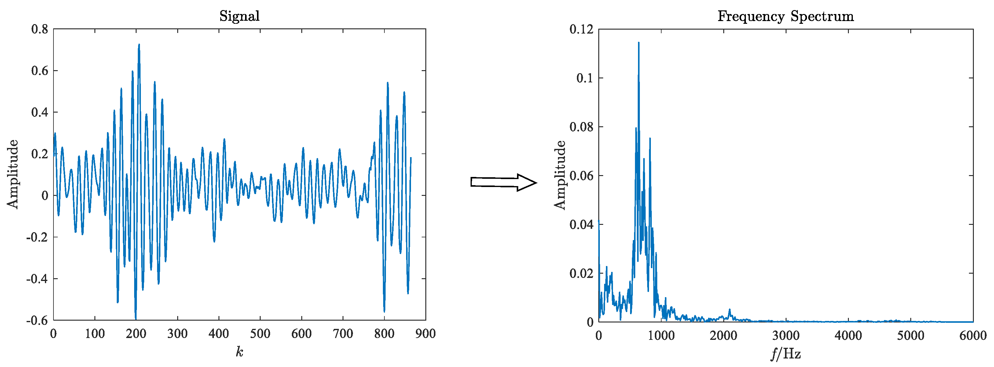
in GST: (1) The original test signal of
dimension is performed FFT, and the
dimension frequency spectrum is obtained. (2) The original test signal of
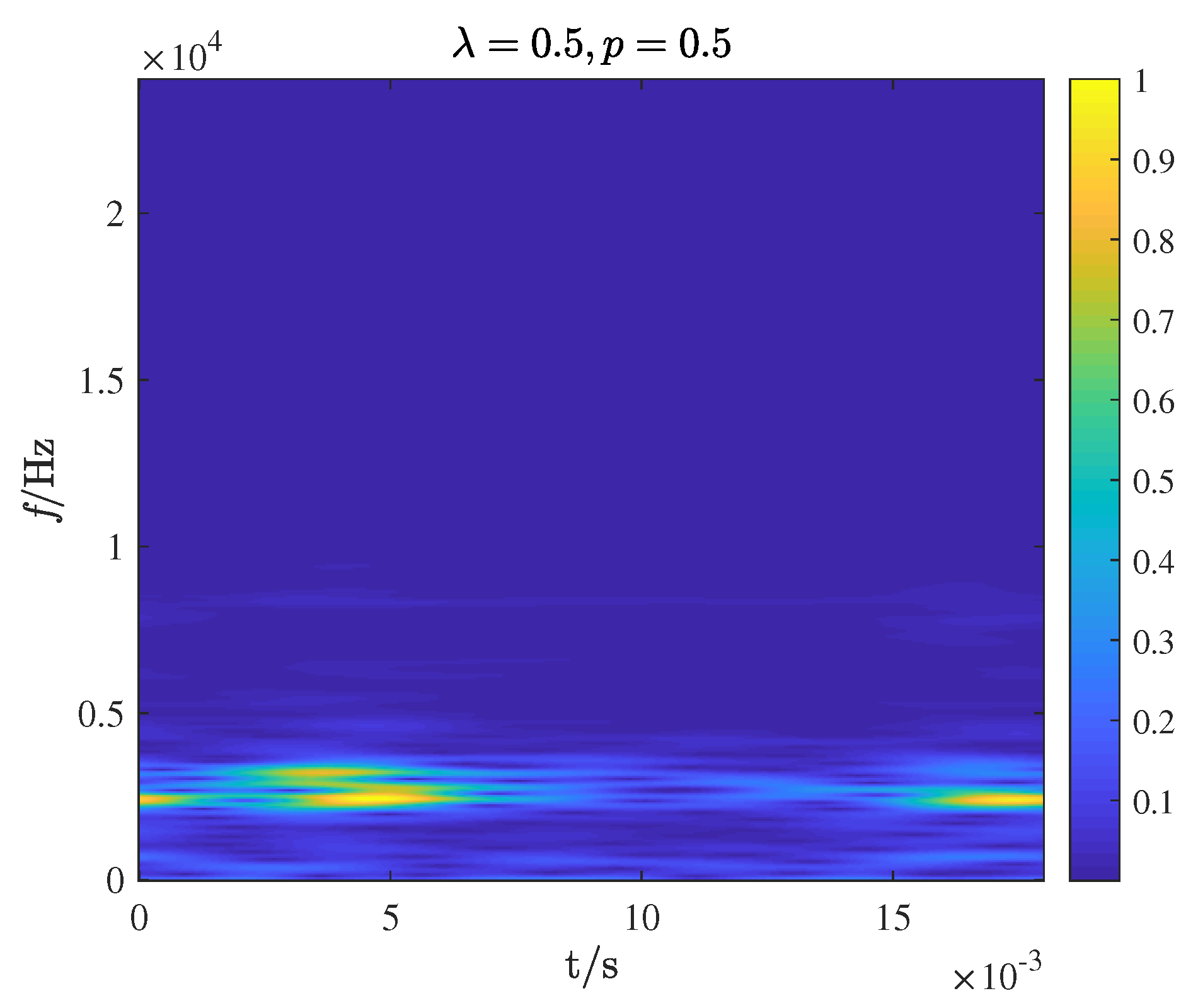
dimension is compressed to a
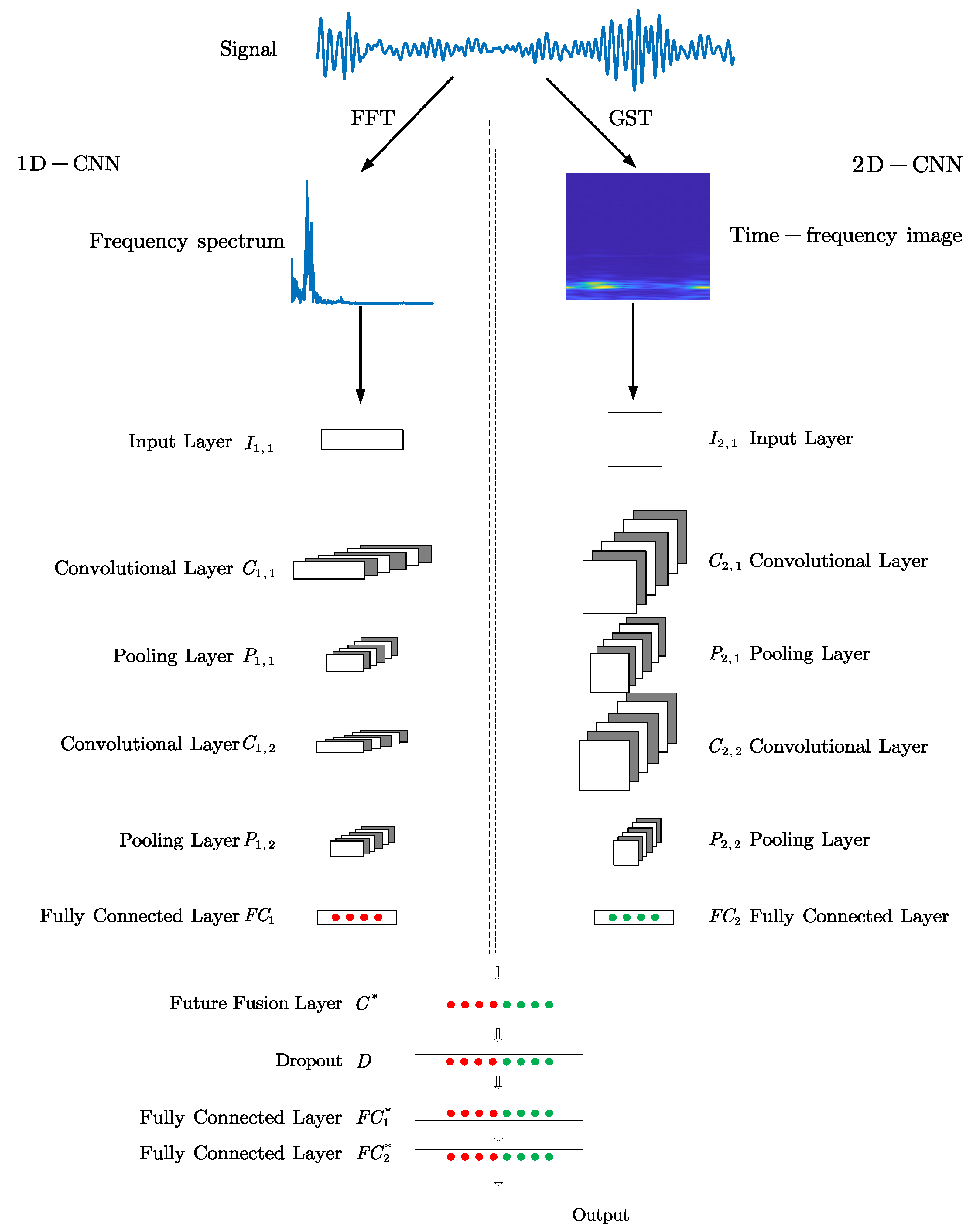
time-frequency image through GST. The purpose of compression is to highlight the primary feature information and not drown out other information, reduce the interference of background information, and improve the proportion of main features. The time-frequency image and frequency spectrum are the input of 2D-CNN and 1D-CNN, respectively. (3) The features extracted from the two CNN models are combined to obtain the final fault features. The network model parameters are obtained based on actual test results. The parameters set for the two networks are shown in
Table 2.
The last fully connected layer is an SVM classifier, and the kernel function is Gaussian kernel. The kernel parameter , and the penalty factor . The remaining parameters are as follows: the dropout ratio is 0.5, the learning rate is 0.005, the mini-batch size is 8, the total epochs is 500, and the loss function is cross-entropy.
4.3. Fault Diagnosis Results under a Balanced Dataset
In addition, 200 samples are randomly constructed for each class, and a sample set containing 2000 samples is constructed. Visualize the hierarchical feature learning process of TC-CNN using the t-distributed Stochastic Neighbor Embedding (t-SNE) method [
41]. The learned features of the original input signal, fully connected layers
, and
of the test dataset are mapped to two-dimensional features using t-SNE, respectively. The mapped features of different layers are shown in
Figure 6,
Figure 7,
Figure 8 and
Figure 9.
Figure 6,
Figure 7,
Figure 8 and
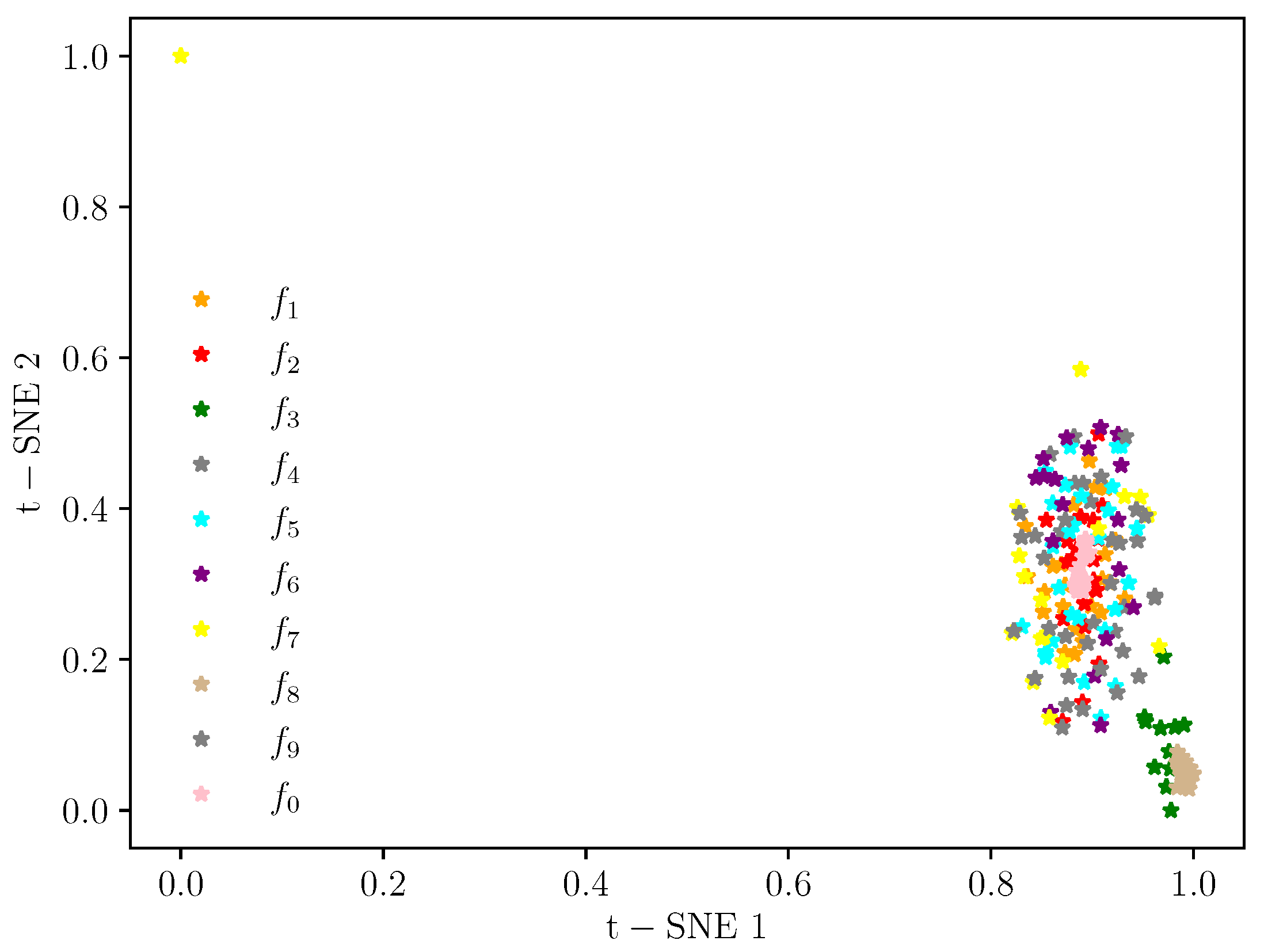
Figure 9 show the feature map changes for different classes during the model learning process. As shown in
Figure 6, the original data features for all classes are relatively scattered and difficult to distinguish.
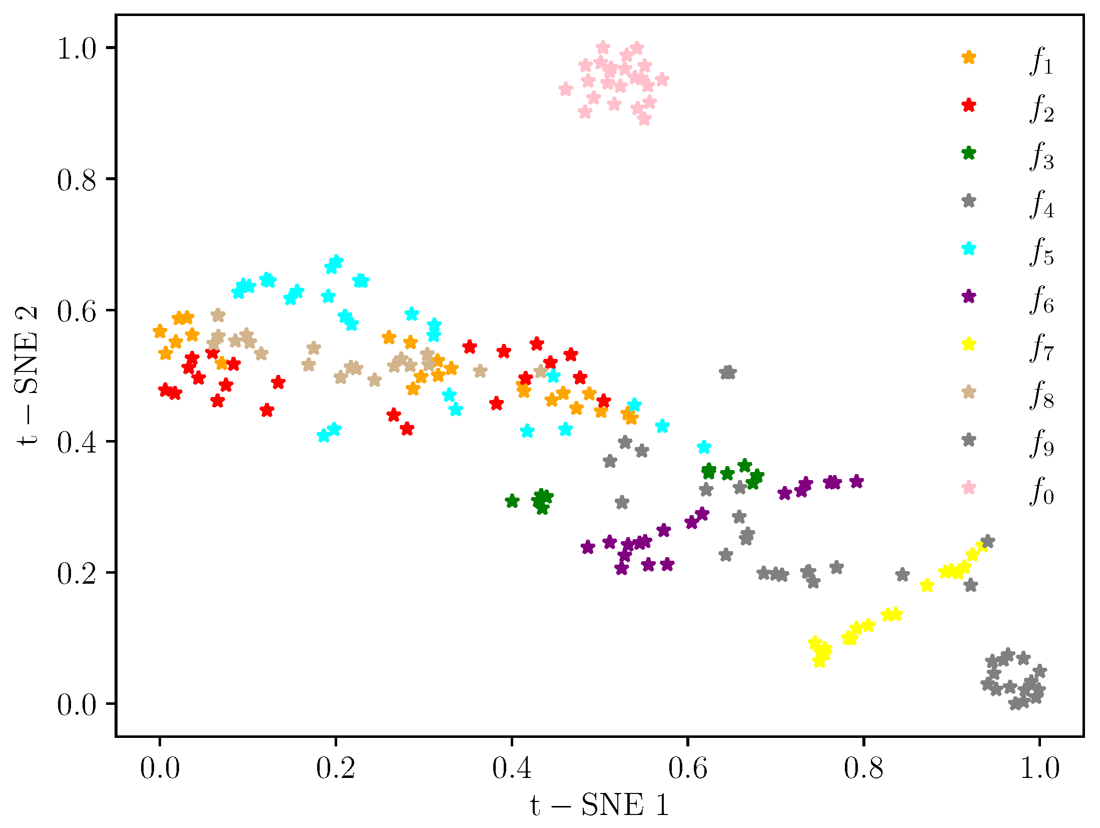
Figure 7 and
Figure 8 show the learned features of the fully connected layers
and
, respectively. Compared with the original input data, it can be seen that, after the convolution and pooling operations, the samples are gradually clustered. Furthermore, the clustering of features in the fully connected layer
is better than that in
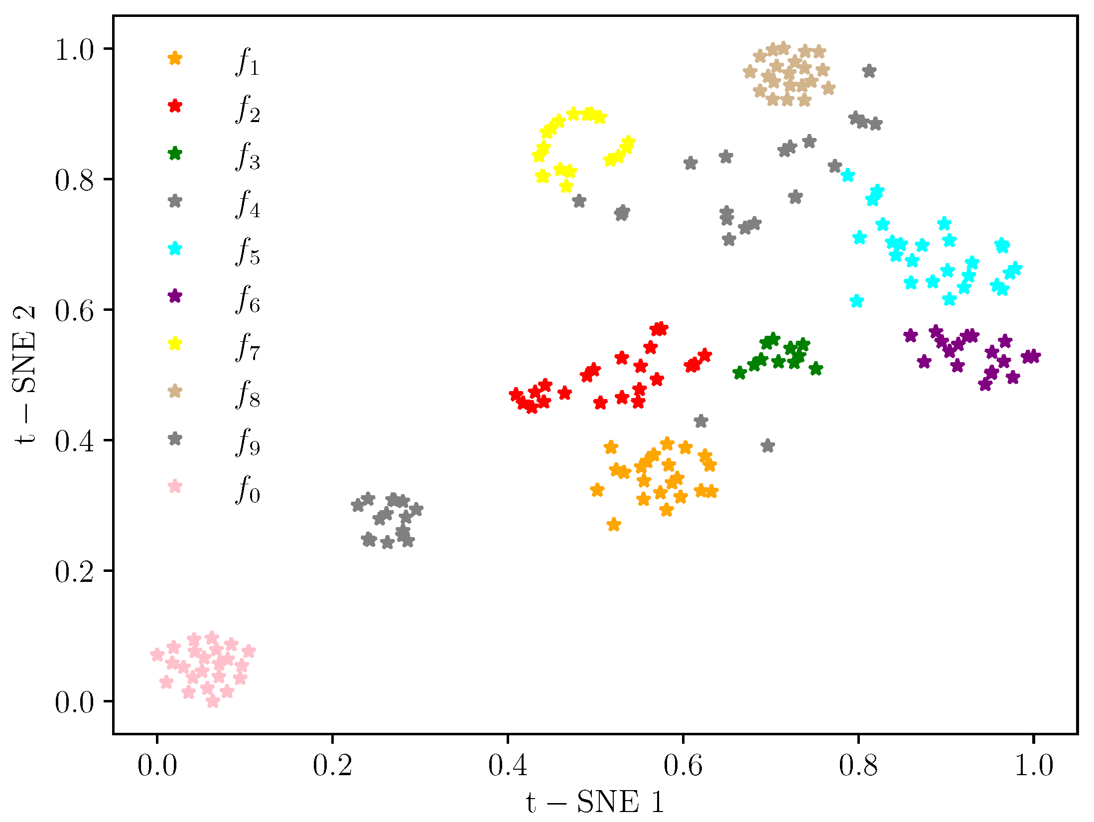
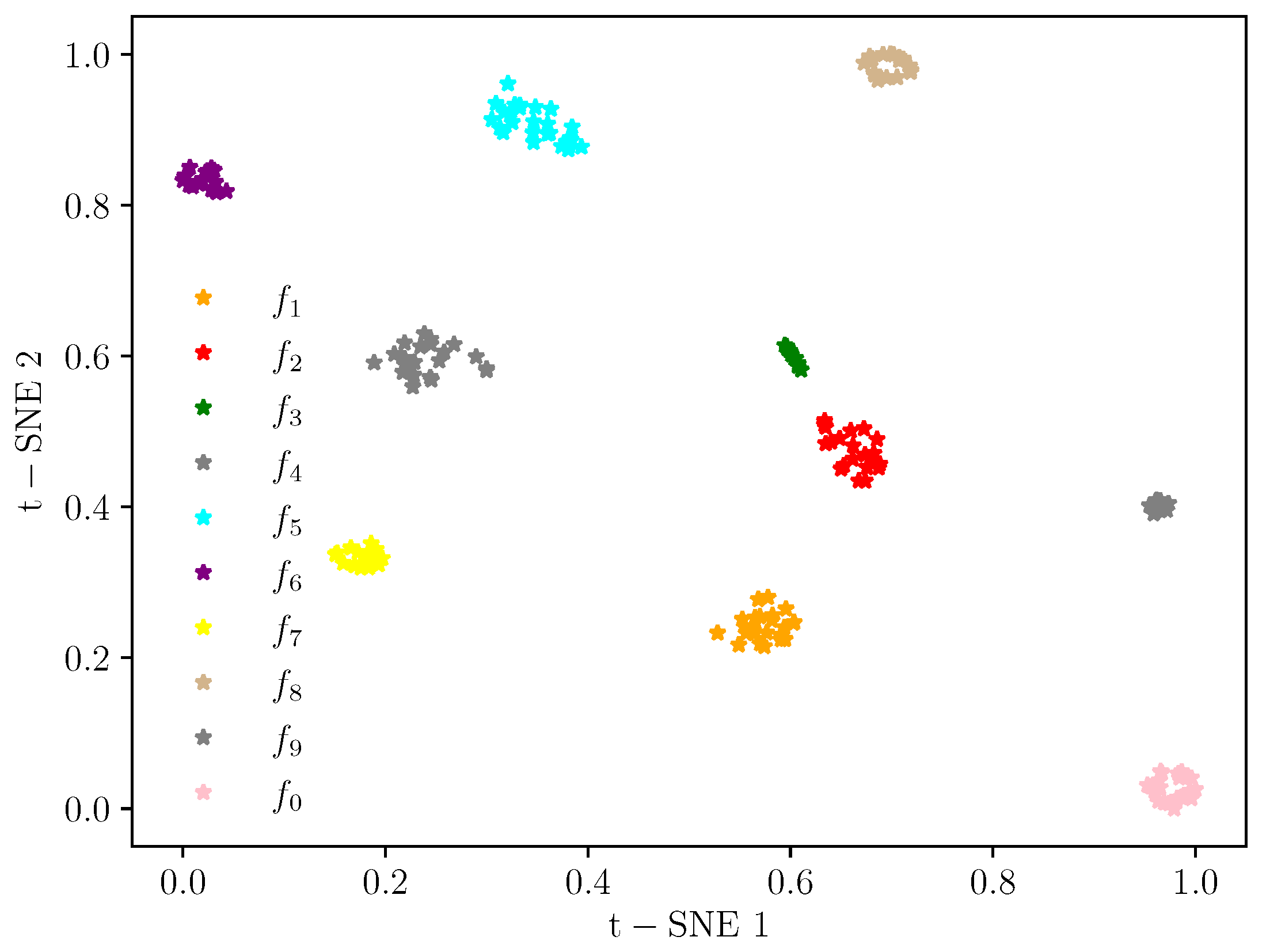
. Finally, in
Figure 9, features of the same class are very concentrated. The distance between the feature distributions in
is the largest compared to the feature mapping results in
and
. The classifier easily performs the classification of the dataset, illustrating the excellent classification results.
The proposed methods in this paper are compared with 1D-CNN, 2D-CNN [
22], CWT+2D-CNN [
38], DBN [
42], and 1D-CNN+2D-CNN.
(1) 1D-CNN consists of an input layer, two 1D convolutional layers, two pooling layers, a fully connected layer, a softmax classifier, and an output layer. The kernel sizes of input and output channels of the convolutional and pooling layers are set as 5, 6, 3, and 6, respectively. The rest of the structural parameters are the same as the 1D-CNN in the proposed model.
(2) Since the dimension of the original signal data are 1024, the original signal data are transformed into a 32 × 32 dimensional matrix as the input of 2D-CNN. The classifier is softmax. The rest of the structural parameters are the same as the 2D-CNN in the proposed model.
(3) CWT+2D-CNN uses CWT to extract the time-frequency features, and the Morlet cmor3-3 wavelet basis function is selected. The CWT time-frequency image is used as the input of the 2D-CNN, and the classifier is softmax. The rest of the structural parameters are the same as the 2D-CNN in the proposed model.
(4) The DBN contains an input layer, two hidden layers, and one output layer, and the network structure is [1024, 50, 20, 10]. The learning rate is 0.05, a mini-batch size is 8, and the number of iterations is 500.
(5) 1D-CNN+2D-CNN has the same network structure as TC-CNN. The difference is that TC-CNN uses FFT and GST to extract features. The inputs of the two channels are frequency spectrum and time-frequency images, respectively. In the 1D-CNN+2D-CNN, the inputs of the two channels are the original signal and the 2D matrix transformed into the original signal, respectively.
To avoid biased results due to random splits of the training and testing datasets,
k-fold cross-validation is applied. All samples are divided into
k mutually exclusive subsets of the same size,
subsets are used as training samples, and the remaining subset is used as testing samples. The training samples are divided into the training set and validation set. A total of
k experiments are performed to obtain
k Accuracy and F1 score results, and the average is taken as the final experimental result. This paper set
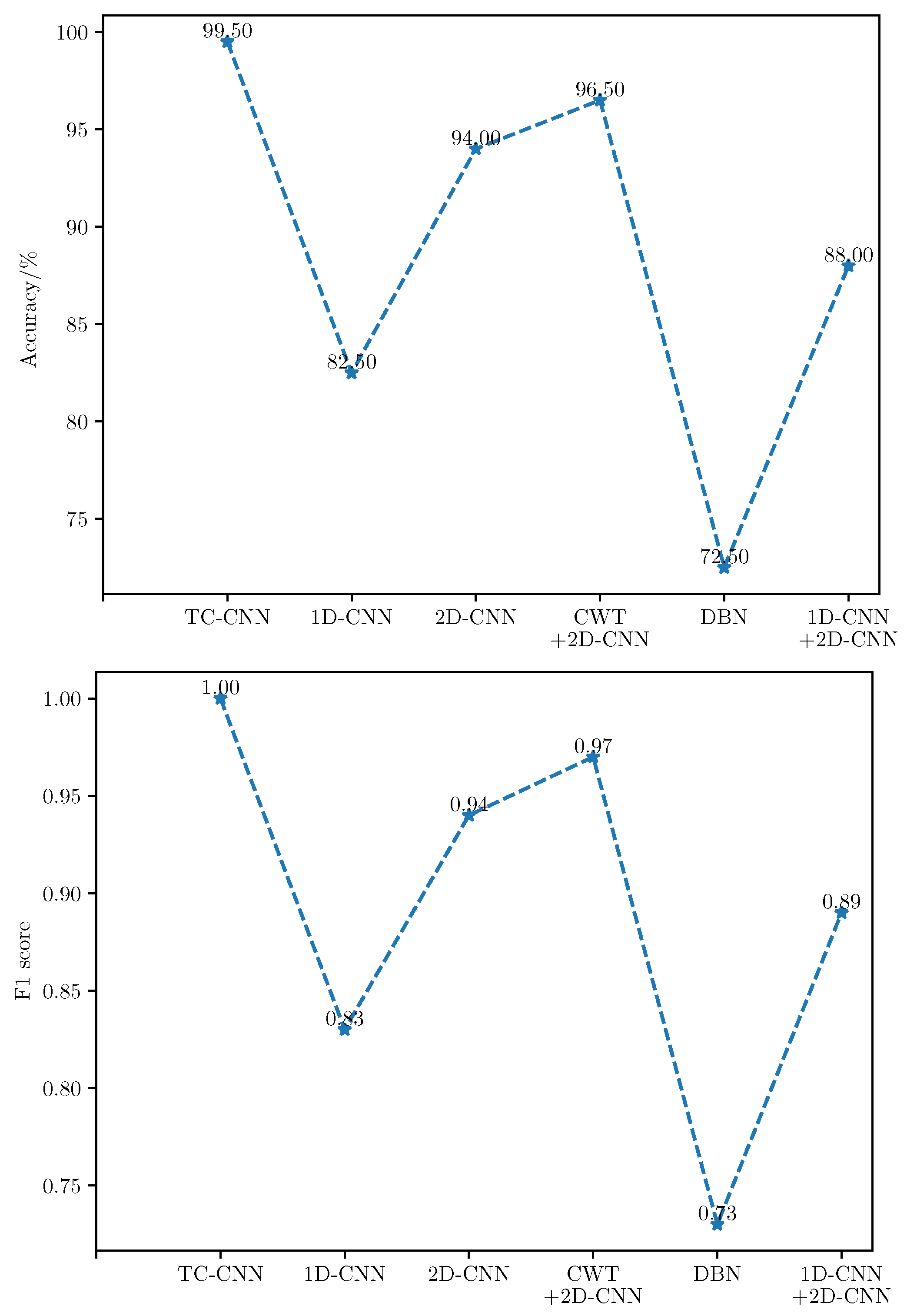
, the sample set is divided into 10 subsets, and the ratio of training set, validation set, and test set is set to: 7:2:1. The Accuracy and F1 score on balanced data samples are shown in
Table 3 and
Table 4 and
Figure 10.
According to the results, it can be found that the methods with convolutional and pooling layers are more capable of fault diagnosis, and the DBN obtains the lowest values of Accuracy and F1 score among these models. Compared with the single-channel CNN model, the fault diagnosis performance of TC-CNN is improved due to information richness. Comparing 1D-CNN with 2D-CNN and CWT+2DCNN shows that 2D-CNN is generally better than 1D-CNN for fault diagnosis. 1D-CNN+2D-CNN also utilizes a two-channel model. Compared with single-channel CNN, its fault diagnosis effect is better than 1D-CNN but worse than 2D-CNN. The reason is that the inputs of both channels are original signals. When the data set is balanced, some extracted features are redundant or unimportant, leading to over-fitting of the model. The diagnostic results of the above-mentioned various models with balanced data sets verify the superiority of TC-CNN.
4.4. Fault Diagnosis Results under the Unbalanced Dataset
The diagnostic performance of TC-CNN is discussed in the previous section based on the balanced datasets. Traditional deep learning models need to be trained with a large number of samples to ensure good performance. In practice, however, the amount of faulty data is very small, and data imbalance is a common phenomenon. Therefore, it is necessary to solve the fault diagnosis problem under unbalanced datasets effectively. In this section, normal data and fault data are mixed in different proportions. The stability of TC-CNN for fault diagnosis is further demonstrated based on the experimental results of the datasets with different proportions. The normal and faulty samples in the training set are mixed in the ratios of 2:1, 5:1, 10:1, 20:1, 30:1, and 50:1, respectively. In the test set, the ratio of normal data to fault data is always 1:1. The distribution of the training set is shown in
Table 5.
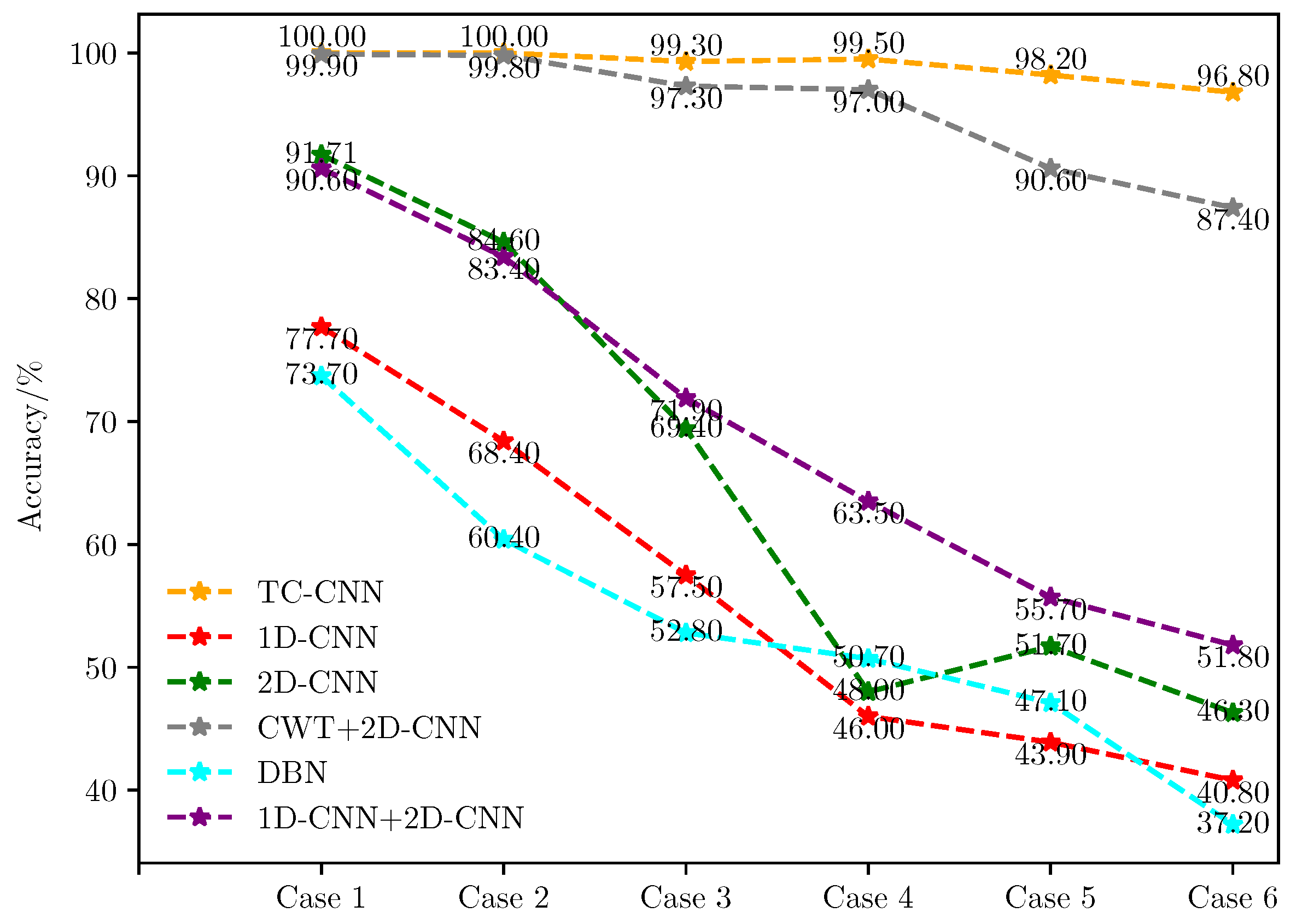
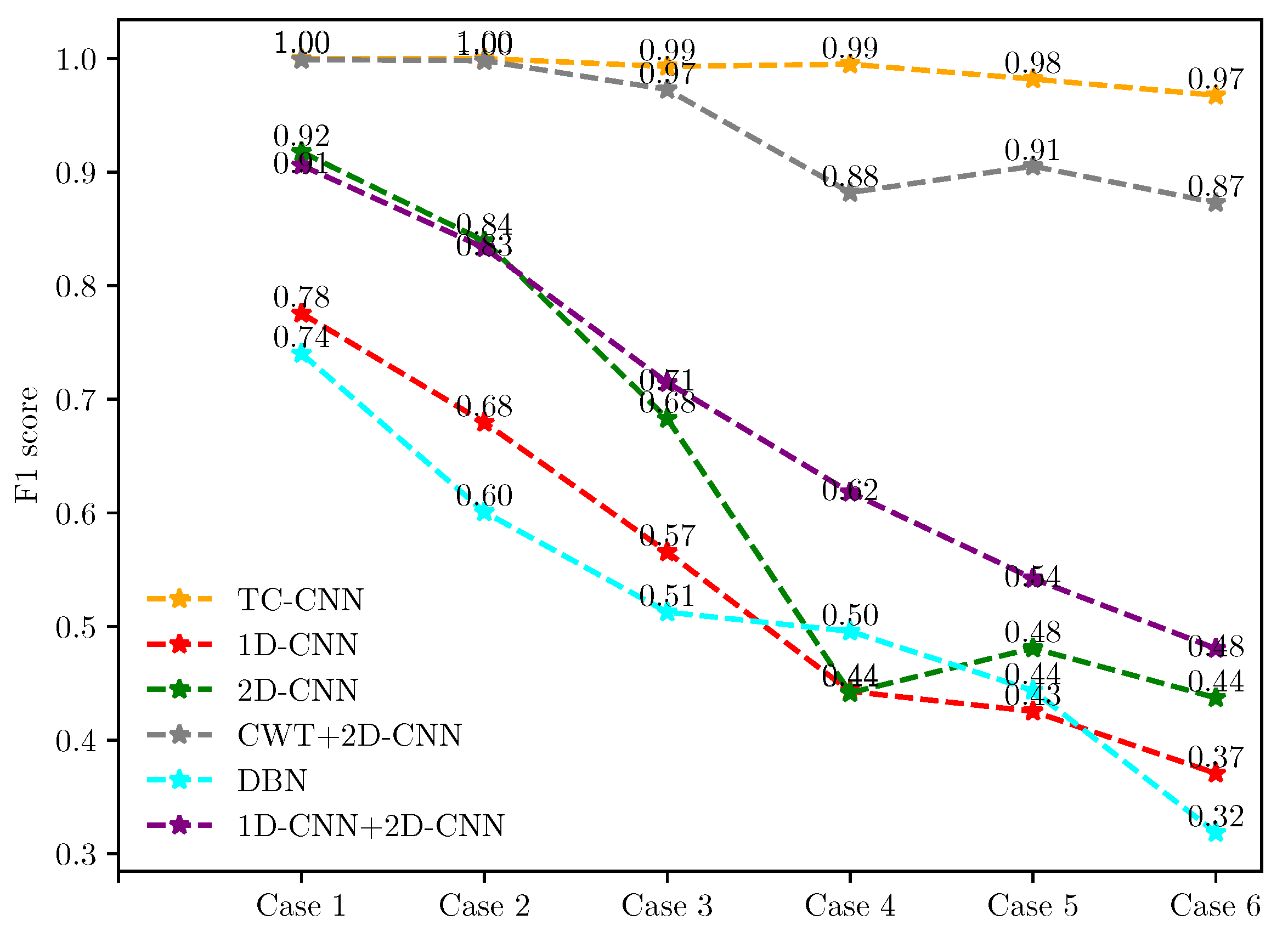
The fault diagnosis results are shown in
Figure 11 and
Figure 12. The fault detection capability of these methods varies with the number of fault samples. In case 1, the diagnostic Accuracy and F1 score for the six methods are (100.00%, 1.00), and (77.70%, 0.78), (91.71%, 0.92), (99.90%, 1.00), (73.70%, 0.74), and (90.60%, 0.91), respectively.
Then, in case 6, the number of faulty training samples is only 1/50 of the normal training samples, and the diagnostic Accuracy and F1 score of the proposed method are 96.80% and 0.97, respectively. The results of other methods are (40.80%, 0.37), (46.30%, 0.44), (46.30%, 0.44), (87.40%, 0.87), (37.20%, 0.32), and (51.80%, 0.48). When the ratio of the number of normal samples to the number of faulty samples reaches 50:1, TC-CNN still has excellent fault diagnosis ability. The diagnostic Accuracy is only 3.20% lower than in case 1, and the F1 score decreases by 0.03. On the contrary, the fault diagnosis performance of the remaining methods decreases significantly with the reduction of the fault sample size. When the fault data in the training dataset decrease as the imbalance rate increases, the model trained by these methods lacks a good ability to identify the fault data in this case. As a result, most of the faulty samples in the test dataset could not be classified correctly, resulting in low Accuracy and F1 score. When the imbalance ratio of data distribution increases, the superiority of the TC-CNN model gradually emerges. The TC-CNN model uses FFT and GST to add fault feature information, which extracts deeply into the data features and makes fault samples easier to distinguish.
When the imbalance ratio is small, such as 2:1, the diagnostic performance of TC-CNN is not much improved compared to CWT+2D-CNN. The feature richness advantage possessed by TC-CNN is relatively small when fault samples are balanced. When the data imbalance ratio is increased from 5:1 to 50:1, the fault diagnosis performance of TC-CNN does not decrease significantly compared with CWT+2D-CNN. Because CWT+2D-CNN only extracts time-frequency features, TC-CNN additionally extracts time-frequency features. The features of different dimensions complement each other, enrich the fault feature information, and make the fault samples easier to identify. When the imbalance ratios are 2:1 and 5:1, respectively, the fault diagnosis performance of 1D-CNN+2D-CNN is slightly lower than that of 2D-CNN. However, as the imbalance ratio gradually increases, the fault diagnosis performance of 1D-CNN+2D-CNN is better than that of 2D-CNN, indicating that 2D-CNN is more susceptible. The reason is that, when training samples are relatively sufficient, 1D-CNN+2D-CNN may extract some redundant features leading to overfitting of the model. However, when the data volume gradually decreases, 1D-CNN+2D-CNN can extract more features that can be utilized and, therefore, has better fault diagnosis performance. The fault diagnosis capability of TC-CNN is significantly stronger than that of 1D-CNN+2D-CNN because FFT and GST can extract more fault information with fewer fault samples, thus attenuating the effect of data imbalance. The training difficulty of DBN gradually increases as the number of training samples decreases, and it cannot effectively represent fault information. In addition, the DBN model has a limited ability to handle noise and other disturbing factors, thus significantly reducing its performance.
Therefore, TC-CNN has better fault diagnosis performance compared with traditional methods, although the severely unbalanced data set leads to performance degradation in all models. In the case of various data imbalance ratios, the TC-CNN model has excellent fault detection results and is less affected by the lack of fault data.


