Regional Analysis of Hotspot and Coldspot Areas Undergoing Nonstationary Drought Characteristics in a Changing Climate

Abstract

Conventional drought indices based on stationary assumptions are no longer appropriate for drought assessments conducted under conditions with climate change or anthropogenic influences. In this study, a time-varying Nonstationary Standardized Precipitation Index (NSPEI) was developed by fitting a time covariate with the Generalized Additive Models for Location, Scale, and Shape (GAMLSS), with a time-scale of six months. Daily precipitation, maximum temperature, and minimum temperature datasets from 1979–2020 that were based on the Climate Prediction Center (CPC) global unified gauge-based analysis with a resolution of 0.5° × 0.5° were used. The results of the study indicated that both precipitation and evapotranspiration in China had increased significantly over the past 42 years in China and that Northwest China would become drier. By extracting the return objects of the GAMLSS, this study identified Northwest China (Continental River Basin) as the main region wherein the distribution parameters of the non-stationary models changed; this region was identified as the one concentrated with nonstationary hotspot response areas. A comparison of drought duration and severity showed that the stationary SPEI under-estimated the severity of the drought. The severity was under-estimated in the spring–summer and fall–winter seasons for Northwest and Southwest of China, respectively; more attention should be paid to these regions. This study provides results that can support nonstationary drought research; droughts can be identified more precisely, and early warnings can be provided for them.

1. Introduction

Multiple factors, such as water pollution, climate change, and population growth, have led to a growing conflict between water supply and demand, resulting in global drought scenarios gaining more attention. Droughts are one of the most complex natural disasters in the world, with impacts on agriculture, society, the economy, and even ecology [1]. Droughts are characterized by their wide area of influence, long duration, and effect on numerous people. Based on historical records, large-scale droughts can be found on all continents, with drought footprints covering North and South America, Australia, Asia, Africa, and Europe [2]. The spatial and temporal distributions of water resources in China are extremely uneven. North and Southwest China experience droughts with the highest frequency and duration [3]. Severe droughts in Southwest China in the fall of 2009 and the spring of 2010 resulted in a lack of potable water for 21 million people and economic losses of $30 billion [4]. Droughts are one of the main threats to agricultural production in Northeast China, and this risk is growing in intensity [5]. Additionally, there are records of droughts causing the Yellow River to dry up.

The difficulty in characterizing droughts stems from the lack of proper understanding of the evolutionary patterns of different droughts [6]. Additionally, information on the precise definition, start, and end of droughts is lacking, providing major obstacles to investigation. Also, the spatial and temporal effects of drought, the instability in their variability, and the anthropogenic factors that trigger droughts are not fully understood [7]. The definitions of a drought are not uniform; a drought can be generally defined as “a prolonged period of abnormally dry weather with scanty rainfall that causes a serious hydrological imbalance [8]”. Traditional droughts can be divided into four categories: meteorological, hydrological, agricultural, and socio-economic [9,10].

A meteorological drought is usually defined as inadequate precipitation over an area for a period of time [1], and it is described by the Standardized Precipitation Index (SPI) and the Standardized Precipitation Evapotranspiration Index (SPEI) [11,12]. A hydrological drought is associated with surface water or groundwater deficits; therefore, runoff data are often used to assess hydrological droughts [10,13]. An agricultural drought is concerned with soil-moisture deficiency with meteorological droughts and climatic factors and their impacts on agricultural production and economic profitability; this drought usually lasts longer than the aforementioned droughts [14]. Droughts have direct and sustained economic and health effects on those engaged in agriculture and indirectly affect non-agricultural populations [15]. Therefore, drought propagation, wherein different types of droughts transform into one another, is possible.

In existing studies, drought conditions are generally assessed using drought indicators, which are prime variables for analyzing the effects of droughts and defining different drought parameters, including intensity, duration, severity, and spatial extent [1]. The Palmer Drought Severity Index (PDSI) [16] and SPI [17] are the most commonly known drought indices. The former is widely used, and the latter is simple to calculate and can be used for different time-scales. With the development of drought research, an increasing number of meteorological and hydro-ecological factors have been added to the assessment of drought indicators. On a precipitation basis, the SPEI [18] and Reconnaissance Drought Index (RDI) [19] consider evapotranspiration. Generally, the Standardized Runoff Index (SRI) [20] and the Surface Water Supply Index (SWSI) [21], which consider runoff, are mostly used to assess hydrological droughts. The Crop Moisture Index (CMI) [22] was used to evaluate agricultural droughts. Furthermore, Mohammad et al. [23] developed a new drought index called the Soil Moisture Drought Index (SODI) based on the quantity of water required to attain soil moisture at field capacity. To assess the ecological impact of droughts, the Normalized Difference Vegetation Index (NDVI) [24,25] is often combined with a drought index to assess environmental droughts.

Conventional drought indices assume stationarity. However, under the combined effects of climate change and anthropogenic influences, such as land-use change [26] and reservoir operations [27], and hydro-meteorological factors, including precipitation, temperature, and runoff not necessarily being stationary, the traditional drought index that is based on the stationary assumption of fixed distribution parameters, ends up being inapplicable in the future [28]. Milly et al. [29] famously asserted that “stationarity was dead”; since then, an increasing number of studies have considered non-stationary factors in the hydrological calculation process.

The Generalized Additive Models for Location, Scale, and Shape (GAMLSS) proposed by Rigby [30] have been widely applied in nonstationary drought assessments. Nonstationarity has been characterized by the construction of linear or non-linear parameters between response variables (drought factors) and explanatory variables (time, climate, and anthropogenic factors) to obtain changes in the distribution parameters [6,31,32]. Including time as a covariate is the most common approach in nonstationary drought models. Considering that a longer time series may contain significant climate change signals, it is not feasible to model time series longer than approximately 30 years using the SPI [33]. Fitting a time-varying gamma distribution to a trending rainfall series makes it possible to attenuate the effect of 100-year precipitation time-series trends on the SPI and reflect more severe and frequent droughts [34]. Wang et al. [35] studied the evaluation of the summer drought in Northern China using the SPI with time as a covariate; the results showed that the non-stationarity of the hydrological time series could not be ignored in drought analyses and forecasts. The nonstationary SPI was superior to the traditional SPI in disclosing the trend of temporal and spatial changes in Southwest China [36]. Similar time-varying nonstationary drought evaluations were conducted using the Standardized Streamflow Index (NSSI) [37,38] and the Non-Stationary Reconnaissance Drought Index (NRDI) [39], and significant differences between the stationary hydrological indices and non-stationary hydrological indices were captured.

With the further developments in research, meteorological and anthropogenic factors have also been introduced into the non-stationary drought assessments. Using climate as a covariate, Li et al. [40] estimated that in Northern China, the Nonstationary Standardized Precipitation Index (NSPI) could capture drought characteristics better than the SPI could; the same results could also be recognized in the middle and lower reaches of the Yangtze River [31]. Kumar et al. [41] explained the non-stationarity of hydro-meteorological variables (precipitation and evapotranspiration) affecting droughts by constructing a GAMLSS-based non-stationary model with a SPEI and a Standardized Deficit Distance Index (SDDI). The climate-driven and human-induced NSSI could provide more reasonable and satisfactory results than the stationary index (SSI) [42]. The NSSI, when used downstream of the Yangtze River, implied the weakening of the reservoirs used to reduce hydrological droughts [38]. As the number of covariates increased, the performance of the nonstationary model improved [32]. Combined with the time-varying copula model, the Nonstationary Meteorological and Hydrological Drought Index (NMHDI) identified more frequent extreme droughts in western China, which could be attributed to its ability to respond to a continuously changing environment [28].

Generally, regional or single-site non-station drought assessments that combine temporal, meteorological, and anthropogenic factors have received widespread attention. However, little attention has been paid to the non-stationarity of evapotranspiration over time due to temperature changes caused by climate change. Most studies on nonstationary drought indicators have focused on a single site and have not reflected the response of the drought index regarding climate change for the entire region of China. To simplify the difficulty of model construction with time as the covariate, GAMLSS were used in this study to construct a linear relationship between the water balance and the covariates with a logistic distribution to obtain the Non-stationary Standardized Precipitation Evapotranspiration Index (NSPEI). The objectives of this study are to (a) identify the hotspot/coldspot areas of the NSPEI in China by classifying the trends of the distribution parameters μ and σ; and (b) compare the drought characteristics identified by the SPEI and NSPEI for the hotspot and coldspot areas, respectively, to obtain the magnitude and the spatial distribution of drought over-estimation or under-estimation under the current stationary drought index. This research can generate accurate drought risk assessments and early warnings regarding situations with climate change.

2. Materials and Methods

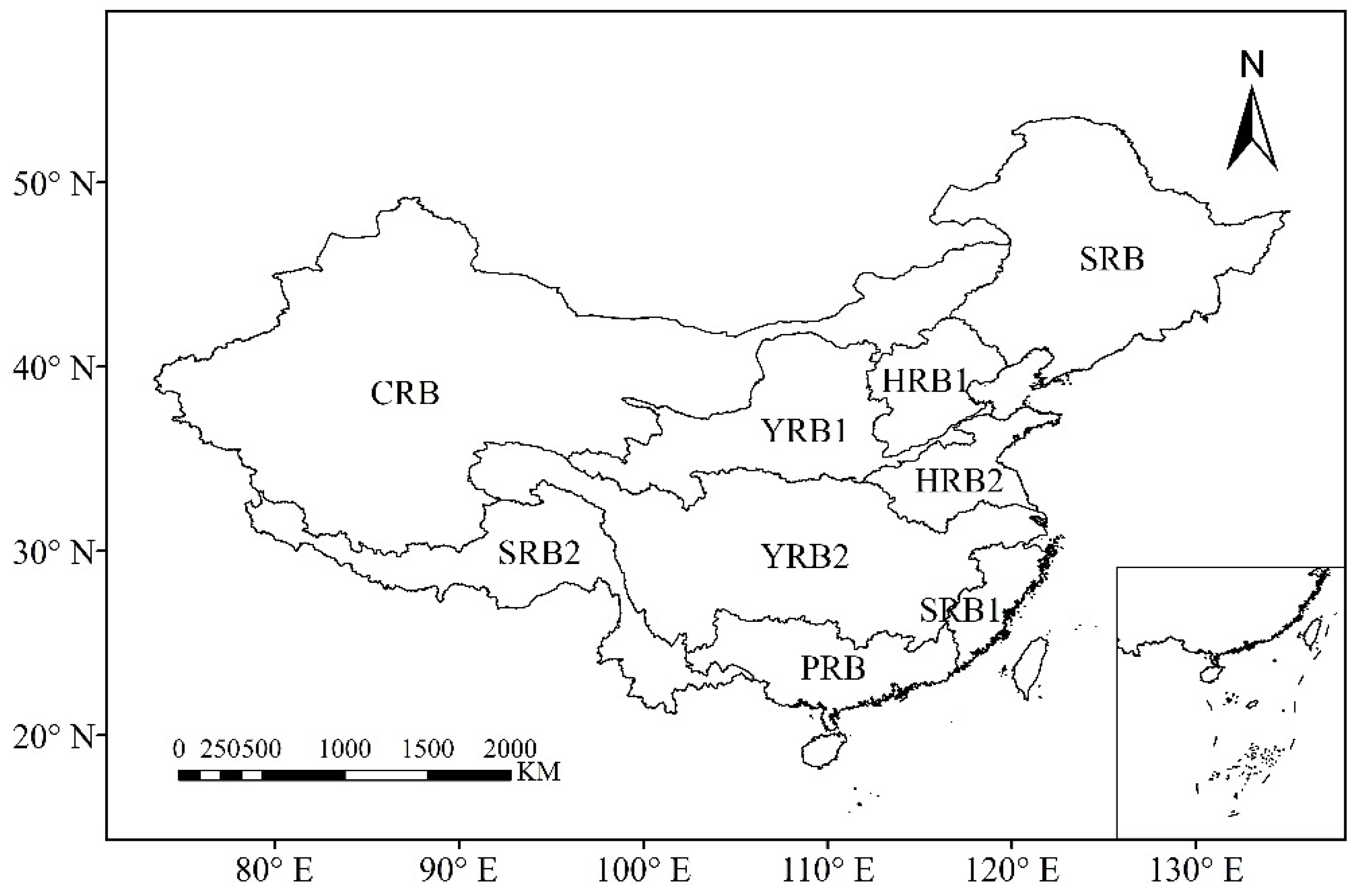
2.1. Study Area

To assess the response of drought to climate change on a national scale, the entire China was selected for this study. As shown in Figure 1, China is a vast country, covering an area of 9,600,000 km² between 3°52′ N–53°37′ N and 73°40′ E–135°05′ E. From the southeast coast to the northwest inland, the average annual precipitation is more than 3000 mm and less than 300 mm, respectively, and the average annual temperature is greater than 35 °C and remains below 10 °C, respectively. Widely varying meteorological conditions have led to different drought conditions in other regions of China.

2.2. Meteorological Data

In this study, under the SPEI, the data used were temperature data and precipitation data [18]. The Climate Prediction Center (CPC) global unified gauge-based analysis of daily precipitation data—having resolution of 0.5° × 0.5° and collected from 1979 to 2020— were used in this study [43]. The CPC global uniform temperature daily maximum and daily minimum temperature datasets were used [44], and the resolution and time-scale were consistent with those of the precipitation data. Before the formal calculation, the monthly total precipitation, the monthly average daily maximum temperature, and the monthly average daily minimum temperature were calculated based on daily precipitation, daily maximum temperature, and daily minimum temperature data, respectively. The monthly average temperature was obtained by averaging the monthly average maximum and minimum temperatures.

2.3. Trend Analysis

In this study, the Mann-Kendall (M-K) [45,46] test, which is the most commonly used nonparametric trend analysis method, was used to evaluate the trend of the initial values, including monthly total precipitation and monthly average temperature. The water balance data was calculated using the difference between precipitation and temperature. Owing to its advantages over parametric statistical testing methods regarding the handling outliers [47], the M-K test is the most appropriate method for analyzing weather tendencies in climatological series [48]. First this test computes the sum of the values as follows:

$$\mathrm{S}={\displaystyle \sum }_{j=1}^{n-1}{\displaystyle \sum }_{i=j+1}^n\mathrm{signal}\left(x_i-x_j\right)$$

(1)

where x_i and x_j are the values of the series, and i and j are the years, respectively; note that i = j + 1.

The signal function can be calculated as follows:

$$\mathrm{signal}=\left\{\begin{array}{c}1, \mathrm{when} (x_i-x_j>0)\\ -1, \mathrm{when} (x_i-x_j<0)\\ 0, \mathrm{when} \left(x_i-x_j=0\right)\end{array}\right.$$

(2)

If n in Equation (1) is too high (>10), then S is normalized. The variance was calculated using the following equation:

$$\mathrm{VAR}\left(\mathrm{S}\right)=\frac{1}{18}\left[n\left(n-1\right)\left(2n+5\right)-{\displaystyle \sum }_{p=1}^q{t}_p\left(t_p-1\right)\left(2t_p+5\right)\right]$$

(3)

where t_p is the fixed number of the data in each group and q is the number of groups.

The Z value can be calculated as follows:

$$\mathrm{Z}=\left\{\begin{array}{c}\frac{S-1}{\sqrt{var\left(S\right)}}, \mathrm{where} (S>0)\\ 0, \mathrm{where} \left(S=0\right)\\ \frac{S+1}{\sqrt{var\left(S\right)}}, \mathrm{where} (S<0)\end{array}\right.$$

(4)

The M-K test was used to determine the confidence level. For a given confidence level, the null hypothesis was accepted when Z was less than Z1 − p/2. In this study, the confidence level was set to 0.01.

2.4. Standardized Precipitation Evapotranspiration Index (SPEI)

Vicente-Serrano et al. [18] proposed a new drought index called the SPEI, which combined the benefits of the SPI [17] being able to respond to multiple time-scales of drought conditions and the Palmer Drought Severity Index (PDSI) [16] accounting for the temperature factor. This proposed index is straightforward to calculate and is based on the original SPI calculation procedure, which uses the difference between the monthly precipitation and monthly potential evapotranspiration (PET). The Thornthwaite method [49], a simple climate water balance method, was used to obtain the SPEI.

The calculation procedure for SPEI is as follows:

(a)

Calculation of the PET; the monthly PET (mm) is obtained by;

$$\mathrm{PET}=16\mathrm{K}{(\frac{10T}{I})}^m$$

(5)

where T is the monthly mean temperature (°C), and I is a heat index, which is calculated as the sum of 12 monthly index values I; i is calculated from the mean monthly temperature using the formula:

$$i={(\frac{T}{5})}^{1.514}$$

(6)

The letter m represents a coefficient that depends on I; $\mathrm{m} =6.75\times {10}^{-7}{I}^3-7.71\times {10}^{-5}{I}^2+1.79\times {10}^{-2}I+0.492$; and k is a correlation coefficient based on the function as follows:

$$k=(\frac{N}{12})\left(\frac{NDM}{30}\right)$$

(7)

where NDM is the number of days of the month, and N is the maximum number of sun hours, which is calculated as follows:

$$N=(\frac{24}{\pi }){\omega }_s$$

(8)

where ${\mathsf{\omega }}_s$ is the hourly angle of the sun rising, which is calculated as follows:

$${\omega }_s=\arccos \left(-\tan \phi \tan \delta \right)$$

(9)

where φ is the latitude in radians and δ is the solar declination in radians, which is calculated using the formula:

$$\delta =0.4093\mathrm{sen}(\frac{2\pi J}{365}-1.405)$$

(10)

where J is the average Julian day of the month.

(b)

(Calculation of the water balance D_i, which is the difference between the monthly total precipitation and monthly PET:

$$D_i=P_i -PE{T}_i$$

(11)

(c)

Calculation of the cumulative difference $D_{m,n}^s\left(t\right)$ in the mth month (January, February, and December) in n years is calculated:

$$D_m^s\left(t\right)={\sum }_{i=k-s+1}^k{D}_i,k=12\left(t-1\right)+m$$

(12)

For the first month, where the order of the D_i series i is smaller than the time-scale s, $D_m^s\left(t\right)={\sum }_{i=1}^k{D}_i$. Note that t = 1, 2, 3, …, n, represents the yearly index.

(d)

Fitting of the cumulative D series using a probability density function. The general optimal distribution of the SPEI has not been specified [50]. To fit the GAMLSS model in R, a two-parameter distribution in the GAMLSS family in R, called logistic distribution, was used in this study ($D_m^s~Logistic(\alpha ,\beta$)).

$$\mathrm{f}\left(D_m^s|\alpha ,\beta \right)=\frac{1}{\beta }\exp \left(\frac{D_m^s-\alpha }{\beta }\right)\frac{1}{{\left(1+\exp \left(\frac{D_m^s-\alpha }{\beta }\right)\right)}^2},-\infty <D_m^s<\infty .$$

(13)

where α and β are the location and scale parameters, respectively.

(e)

Fitting of the cumulative probability of the D series under a particular time-scale is fitted. By transforming the cumulative probability density into a standard normal distribution with a mean of zero and variance of one, the SPEI can be obtained.

A time-scale of six months was chosen in this study. Since the calculation of the SPEI index was based on that of the original SPI [18], the definition of the drought intensity of the SPEI was consistent with that of the SPI. The threshold values of the SPEI index and their corresponding drought levels are shown in

Table 1. Threshold values of the SPEI index classification.

Threshold Value	Description
SPEI > −0.50	Normal
−1.00 < SPEI ≤ −0.50	Mild drought
−1.50 < SPEI ≤ −1.00	Moderate drought
−2.00 < SPEI ≤ −1.50	Severe drought
SPEI ≤ −2.00	Extreme drought

.

A drought event for each time-scale is defined as a period wherein the SPEI is continuously negative, reaching a value of −1.0 or less [17]. The definition of a complete drought event should include the start time, ending time, duration, and intensity at each time point. In this study, the duration was defined as the months for which a drought event lasted from beginning to end. The intensity was defined as the absolute value of the SPEI value for each month. The severity of a drought event was defined as the cumulative intensity value within the drought duration.

2.5. GAMLSS Approach

The GAMLSS proposed by Rigby and Stasinopoulos [30] were chosen to describe the relationship between drought factors and explanatory covariates. These are widely used nonstationary models for hydro-meteorological elements [28,31,35,39]. GAMLSS are univariate distributional regression models, wherein all the parameters of the assumed distribution for the response can be modelled as additive functions of the explanatory variables through linear or nonlinear functions.

The principle of the GAMLSS model is as follows.

In the GAMLSS, the times series y_i, where i = 1, 2, …, n follows the probability density function $\mathrm{f}\left(y_i|{\theta }^i\right)$ conditional on ${\theta }^i=\left({\theta }_{1i},{\theta }_{2i},\dots ,{\theta }_{oi}\right),$ where ${\theta }^i$ is the vector of the o para meter of the distribution. Let $y^T=\left(y_1,y_1,\dots ,y_n\right)$ be the n-length vector of the response variables in the observations. For $\mathrm{k} =1,2,\dots ,p, J_k=0,$ a fully parametric model for ${\mathrm{g}}_k\left(·\right)$ is a known monotonic link function relating ${\theta }_k$ to the explanatory variable and random effects through an additive model given by:

$${\mathrm{g}}_k\left({\theta }_k\right)={\eta }_k=X_k{\beta }_k+{{\displaystyle \sum }}_{j=1}^{J_k}{h}_{jk}\left(x_{jk}\right)$$

(14)

where ${\theta }_k$ and ${\eta }_k$ are vectors of length n, $X_k$ is a matrix (n × m) of the explanatory variables, and ${\beta }_k$ is a parameter vector of length m. The function $h_{jk}\left(·\right)$ is an unknown function of the explanatory variable $x_{jk}$ for $j=1,2,\dots ,J_k$ and $k=1,2,\dots ,p$. Equation (14) represents a semiparametric model, wherein the first two population parameters ${\theta }_1$ and ${\theta }_2$ are usually characterized as location and scale parameters, denoted by μ and σ, respectively, whereas the remaining parameters, if any, are characterized as shape parameters.

Two basic algorithms were used for maximizing the penalized likelihood: the Conjugate Gradient (CG) algorithm [51] and the Rigby and Stasinopoulos (RS) algorithm [52,53]. The RS algorithm was easy to implement and has been successfully used for fitting all the distributions, including the logistic distribution. The Akaike information criterion (AIC) [54] was used to evaluate the goodness of fit and avoid model overfitting.

$$\mathrm{AIC} =2\mathrm{l} -2\ln (\widehat{L})$$

(15)

where l is the number of estimated parameters in the model, and $\widehat{L}$ is the maximum value of the likelihood function of the model. All computations in this study were performed with the GAMLSSS R package available from the Comprehensive R Archive Network (CRAN) of the R library.

2.6. Nonstationary Standardized Precipitation Evapotranspiration Index (NSPEI)

The SPEI index assumes that the probability distribution of the Di series is stationary, meaning that the parameters do not change over time; however, the hypothesis may not be true in a changing climate. In this study, we propose using the NSPEI with the time covariates and GAMLSS; both the location and scale parameters changed over time with a linear function. The nonstationary model of $D_m^s$ can be represented as follows:

$$\begin{array}{c}{D}_m^s\left(t\right) ~ Logistic\left(\alpha \left(t\right),\beta \left(t\right)\right)\\ \alpha \left(t\right)=a+bt\\ \beta \left(t\right)=c+dt\end{array}$$

(16)

where a, b, c, and d are the constants that need to be estimated in the GAMLSS.

NSEPI and SPEI share similar calculation principles; thus, the levels of drought classification under the NSPEI followed those under SPEI, which are shown in Table 1.

3. Results

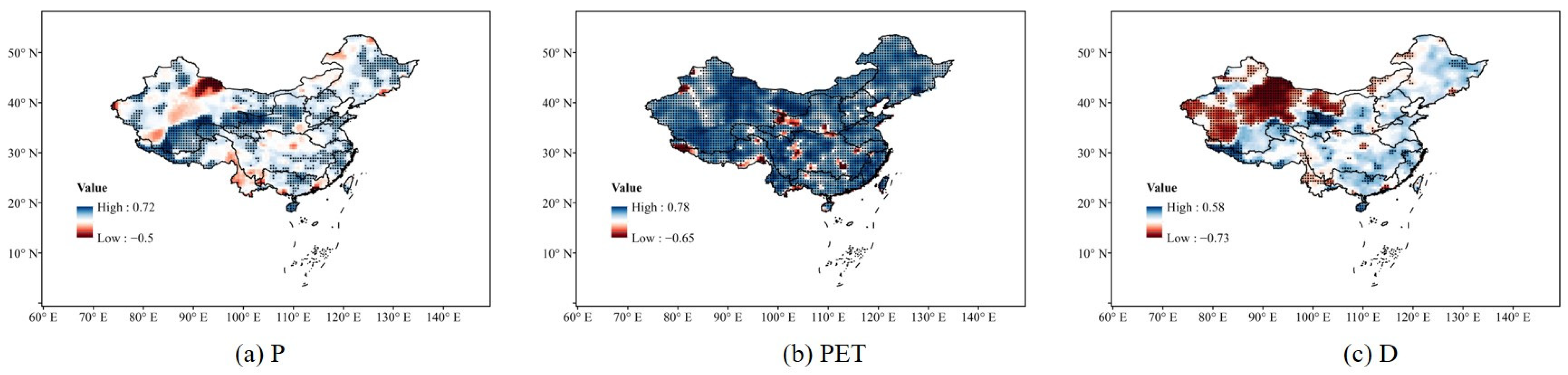
3.1. Spatial and Temporal Distribution of Long-Term Trends in Meteorological Variables

The spatiotemporal distribution of the long-term trends of the P, PET, and D series estimated by the M-K trend test is shown in Figure 2, where blue indicates an increasing trend, red indicates a decreasing trend, and black dots represent 95% and higher confidence levels. The annual and monthly trends for 1979–2020 were computed for all the variables at all the grid points. As shown in Figure 2, except for the Southeast of China and a small region of the northern CRB, most of the area shows a slightly increasing trend of precipitation with the grid points in the Qinghai–Tibet Plateau, YRB1, and Eastern China reaching confidence levels of 95% and more. Regarding evapotranspiration, almost all of China showed a significantly increasing trend. This suggested that it was essential to consider evapotranspiration in drought assessment because if only precipitation was focused on, future droughts would likely to be misjudged in terms of severity. The D series, which was calculated as P-PET, showed a significantly decreasing trend in Northwest China and a negligibly increasing trend in other regions of China. Figure 2 shows that Northwest China may become even drier. Given that climatic conditions have changed over 42 years, the traditional drought assessment index is no longer applicable under current conditions of climatic changes, and, thus, a nonstationary drought index needs to be developed.

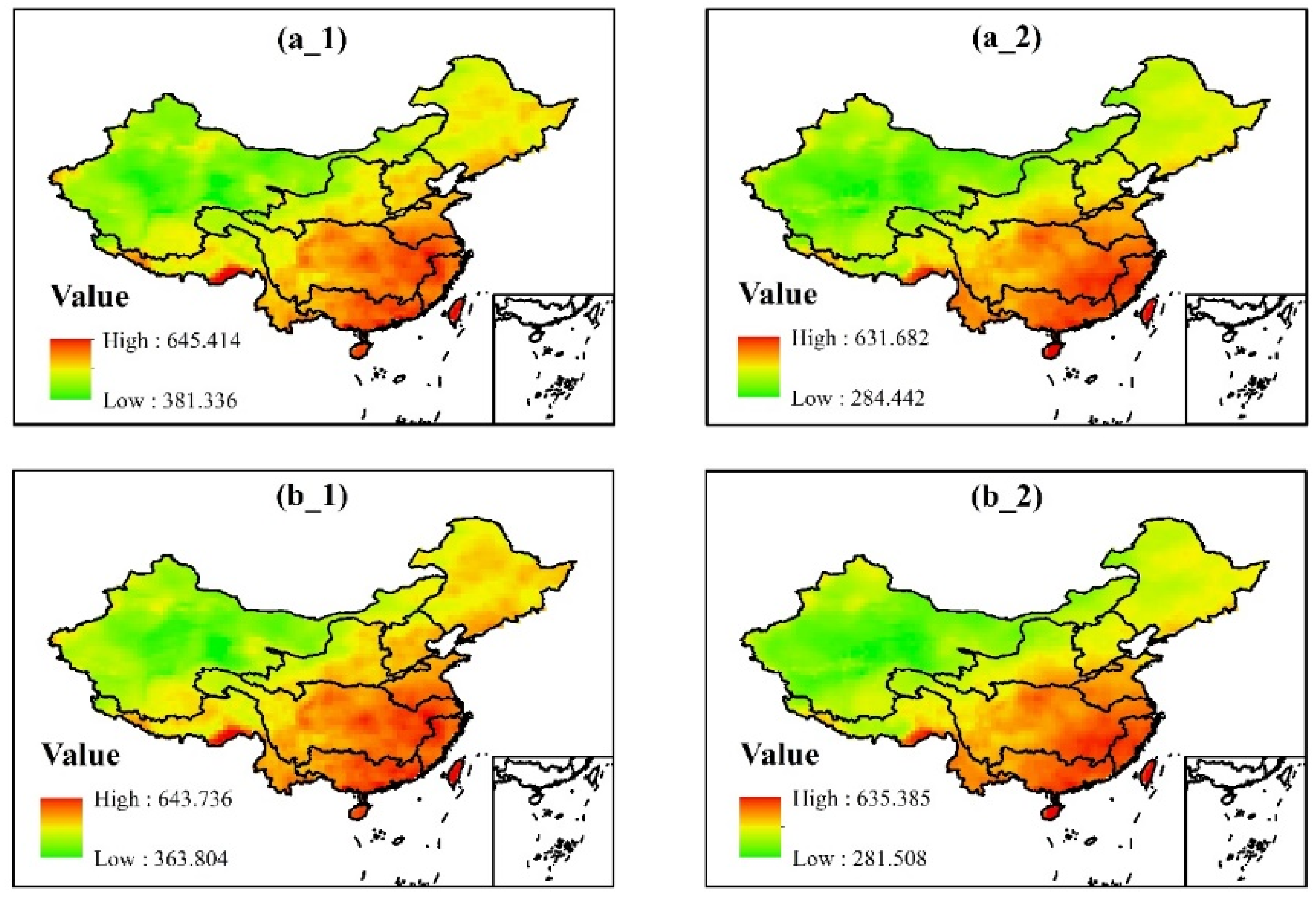
3.2. Performances of Nonstationary and Stationary Models

Figure 3 shows the performance of the non-stationary and stationary models evaluated using the AIC for the eighth month (D series fitted with GAMLSS for the spring–summer season) and the second month (D series fitted with GAMLSS for the fall–winter season). The spatial distribution of the different models is consistent across the months, consistently showing a trend of decreasing AIC values from the southeast to northwest, which implies the optimization of the model performance.

The AIC values are in the range of 300–600 for both the non-stationary and stationary models, proving that nonstationary models have qualified simulation results similar to those of the stationary model. The simulation performance of the nonstationary model in Southeast China is similar to that of the stationary model; it is slightly better in Northeast China, especially in the CRB. Combined with the long-term change of the D series, Northwest China reacts strongly to climate change, and a nonstationary model with precipitation and temperature climate covariates is needed for a better evaluation of the drought conditions.

3.3. Nonstationary Hotspot Response Areas

When using the GAMLSS for constructing a six-month scale nonstationary SPEI, the linear fitting results of the location and scale parameters of the fitted covariates are examined based on the model coefficients extracted from the return objects of the modeling function (Figure 4). There are four types of (μ, σ) values at the 95% confidence level, namely (0, 0), (1, 0), (0, 1), and (1, 1), indicating no change in either parameter, change in location parameter, change in scale parameter, and changes in both parameters, respectively.

Figure 4 shows that for both the eighth month—wherein the D series if fitted with GAMLSS for the spring–summer season—and second month—wherein the D series is fitted with the GAMLSS for the fall–winter season; the change analysis of the distribution parameters shows the change in the location parameters in Northwest China, no change in other regions, sporadic changes in regional scale parameters, or changes in both the parameters. This means that Northwest China as well as some sporadic regions distributed in Central and Southwestern China are the nonstationary hotspot response areas. In the region where the location and scale parameters show no significant trend, the drought conditions estimated by the NSPEI and the SPEI may generally be consistent because almost no distribution parameters have changed over the past 42 years. However, the drought conditions estimated by the NSPEI and SPEI need to be further analyzed in relation to the changes in the distribution parameters. In the next section (Section 3.4), the drought characteristics computed by the SPEI and NSPEI under different classifications of distribution parameters and river basins are compared.

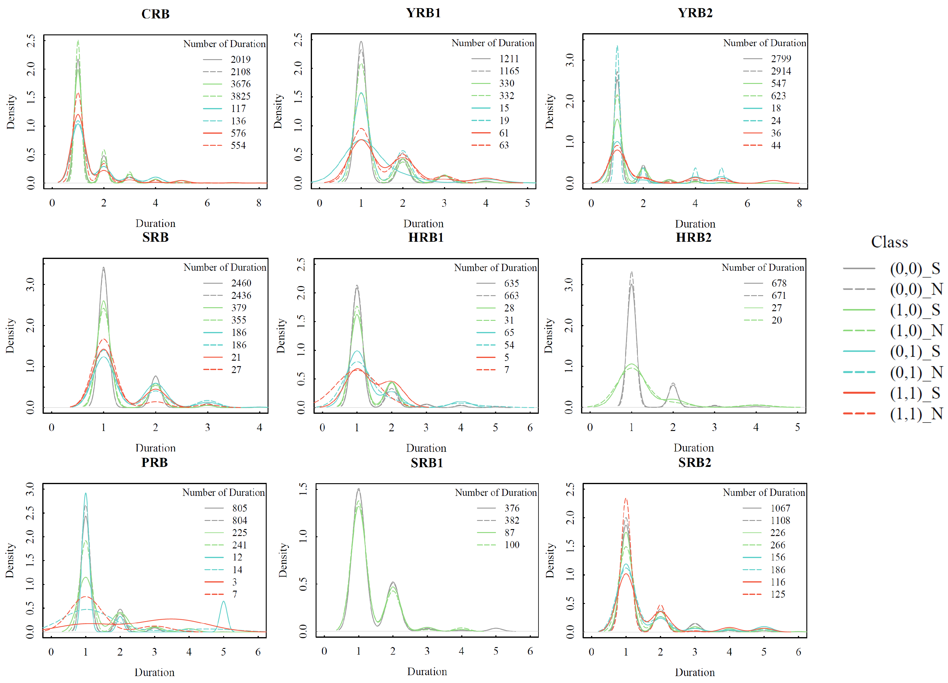
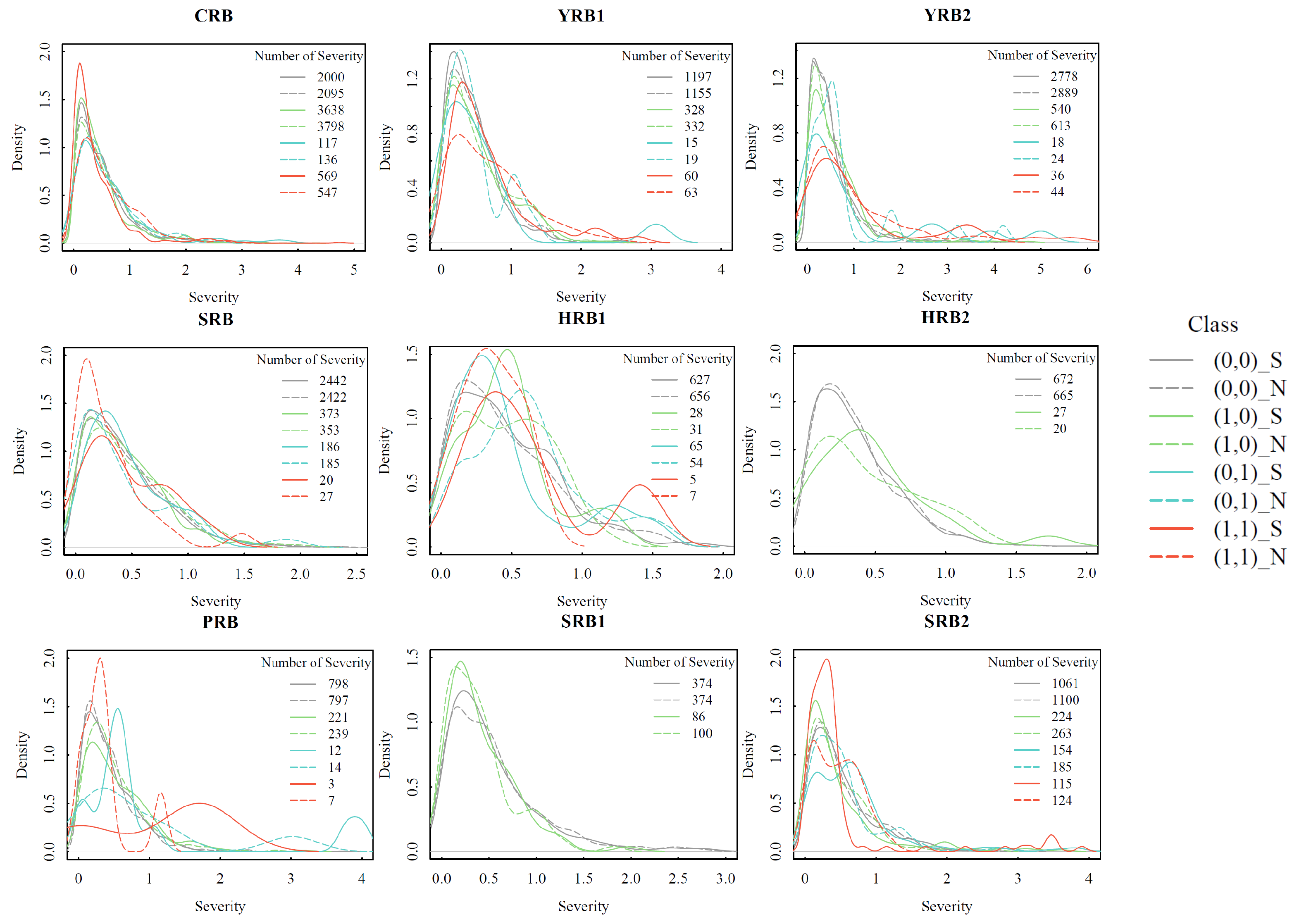
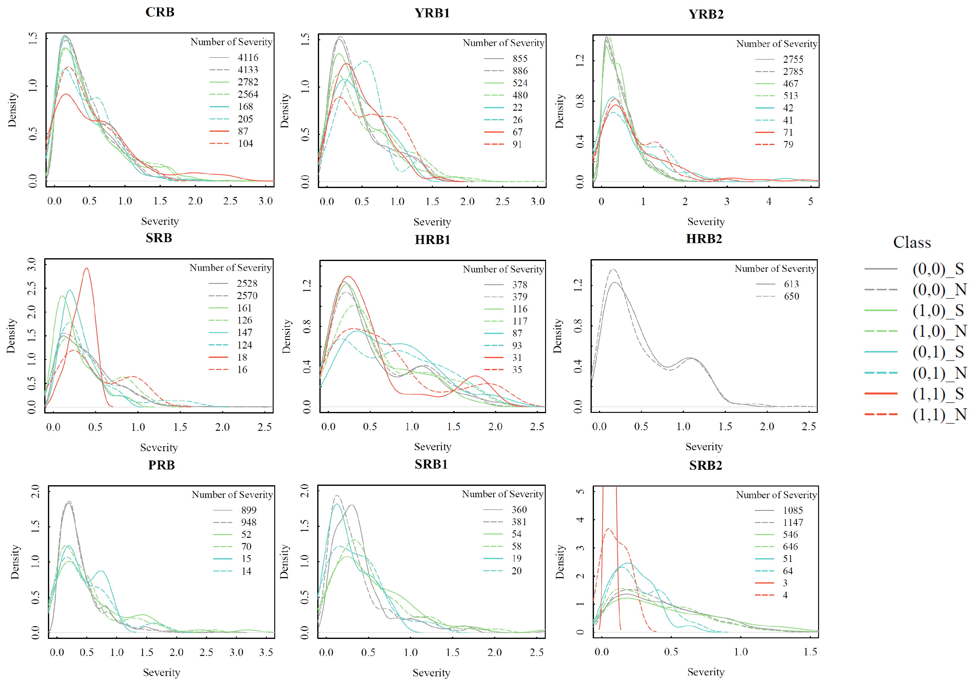
3.4. Comparison of Nonstationary and Stationary Drought Characteristics in China

Figure 5 shows the percentage of the differences in drought characteristics estimated using the NSPEI index and SPEI. The differences are represented as $\frac{DrouCha{r}_{NSPEI}-DrouCha{r}_{SPEI}}{DrouCha{r}_{SPEI}} \times 100\%$; the values of the drought characteristics estimated by the SPEI are subtracted from those of the drought characteristics (duration and severity) estimated by the NSPEI as a percentage of the drought characteristics estimated by the SPEI. Positive values imply an under-estimation of the drought conditions by the current stationary index and vice versa. Figure 5 shows that in many areas of China, the results of the SPEI and NSPEI are the same (shown in white). The differences in these indices were concentrated between −15 and 15%, and these differences were spatially dispersed. Overall, the differences between the stationary SPEI and NSPEI values for the drought durations were minor, and there was no obvious spatial pattern.

For drought severity, drought assessment generally remained consistent in the east during the spring–summer season, while in sporadic areas, such as the YRB2, Eastern SRB2, and PRB, there was over-estimation of drought severity under the stationary SPEI. The same results could be found in the fall–winter season, except for a more visible underestimation of drought severity in the southeast and the HRB1. The most significant difference in drought evaluation between the nonstationary and stationary models was found in Northwest China, that is, the CRB. The under-estimation of drought by the stationary SPEI in this region was particularly evident during the spring–summer season, while the over-estimation in the eastern sheet and northern ribbon regions could also be observed. In the fall–winter season, the over-estimated area expanded, and the under-estimated area decreased. This may be due to the decrease in precipitation and increase in evapotranspiration during the spring–summer seasons in the region, while there was no significant change in precipitation and reduced or no evapotranspiration during the fall–winter seasons (Supplementary Figures S1 and S2).

Figure 6, Figure 7, Figure 8 and Figure 9 show the probability densities of drought characteristics (duration and severity) evaluated using the SPEI and NSPEI under the classification of different changes in the distribution parameters (μ, σ) in different river basins during the spring–summer and fall–winter seasons for all the grid points. Figure 6 shows the results of the durations for the spring–summer season. The results of the NSPEI and SPEI assessment only varied in the distribution of durations; there was no probability bias. As mentioned in the previous section, the results of the nonstationary and stationary models were essentially indistinguishable for the case wherein the distribution parameters presented (0, 0) variations. For the (1, 1) class, the nonstationary index identified more durations in all the river basins than the stationary index did. There were only a few grid points where only the scale parameter changed (class of (0, 1)), and the drought durations identified by the NSPEI and SPEI were similar. Variations in the (1,0) class were identified only at grid points close to Northwestern China, such as CRB, YRB2, YRB1, and SRB2. The results showed that stationary approaches under-estimated the drought duration in the spring–summer season for the past 42 years. The CRB requires further attention, as most of the grid points with changes in the distribution parameters are concentrated here.

The drought severity evaluated by the NSPEI and SPEI shows some variation not only in the distribution of the severity but also probability density (as shown in Figure 7). For the CRB, where there are the main hotspots of nonstationary response areas and the most grid points showing changes in the distribution parameters (μ, σ), the stationary SPEI not only quantitatively under-estimated drought severity, but also identified some of the more severe droughts as less severe. In other river basins in China, the (0, 0) class has shown consistent drought evaluation results for the past 42 years in the spring–summer season. Numerically, the SPEI and NSPEI assessed the severity similarly, but for some grid points, the stationary SPEI over-estimated the severity of ones with smaller severity while under-estimating that of ones with larger severity.

As with the spring–summer season in Figure 8, the drought duration also shows only quantitative differences in the fall–winter seasons; there is no probabilistic bias, and the differences are small. The stationary SPEI seemed to over-estimate the drought duration in river basins, such as CRB, YRB1, YRB2, and SRB, which had more grid point variations in the location parameters (1, 0); while under-estimating the drought severity in the river basin SRB2 because there was little evapotranspiration in Northwest China during the fall–winter season. Therefore, drought conditions considered nonstationary seemed to ease while significant precipitation decreased, and evapotranspiration increased in Southwestern China during this season (shown in Supplementary Figures S1 and S2). The nonstationary and stationary results of the (0, 1) class exhibited only minor differences. The grid points of the (1, 1) class accounted for a small number and indicated an under-estimation of drought severity, as in the spring–summer season. The same results for severity are shown in Figure 9. For river basins, such as CRB, YRB1, SRB2, and HRB1, that had more variable grid points for the distribution parameters, there was under-estimation under the stationary SPEI for droughts of greater severity.

Generally, in the cases wherein there were no changes in either parameter (0, 0) or only a change in the scale parameter (0, 1), the nonstationary or stationary model evaluated the same drought event, whereas there was under-estimation under the stationary SPEI in the case wherein there were both location and scale parameter changes (1, 1). Under the combined effect of precipitation and evapotranspiration changes, the traditional stationary SPEI under-estimated the drought in Northwest China during the spring–summer season; and then, under-estimated it in Southwest China in the fall–winter season. Meanwhile, the stationary SPEI under-estimated the occurrence of drought events with longer durations and greater severity in China, possibly resulting in the inadequate identification of severe or even extreme droughts under conditions of climate change.

4. Discussion and Conclusions

Conventional drought indices that work based on stationary assumptions are no longer suitable for characterizing drought under the influence of factors, such as climate change or anthropogenic influences. Thus, in this study, we applied a six-month scale NSPEI with t covariates using GAMLSS to identify hotspot areas in China that were sensitive to nonstationary models. By comparing the drought characteristics (duration and severity) of the stationary model and nonstationary models, this study investigated the over-estimation or under-estimation of droughts using the current stationary SPEI index under four classifications of changes in distribution parameters.

Long-term trends in precipitation and temperature in China during the period 1979–2020 indicated that precipitation had increased in China over the past 42 years, with the increase in temperature being more pronounced. This was consistent with the findings of Sun et al. [55] for a warming environment. Wu et al. [56] identified an increase in precipitation in Western and Southeastern China between 1960 and 2020; the evapotranspiration, which was assessed using the Thornthwaite formula, has increased significantly over the past 42 years. These results revealed that both evapotranspiration and nonstationarity needed to be considered in drought assessment because if only precipitation was focused on, the severity of the drought would be misjudged as less severe, and if nonstationary was not considered, the changes produced would not be accurately captured. The change in the D series suggested that Northwest China would become drier.

Using the AIC, we obtained good fits for both the nonstationary and stationary models. From Southeast to Northwest China, the AIC values decreased, indicating a better model performance. Based on the model coefficients extracted from the return objects of the GAMLSS, four types of location (μ) and scale (σ) parameter changes under a 95% confidence level were obtained: (0, 0), (1, 0), (0, 1), and (1, 1). This study selected the results of the second and eighth months from the GAMLSS, which represented the spring–summer and fall–winter seasons, respectively. The analysis results showed that Northwest China (CRB) was the main region wherein the distribution parameters varied; it was the main nonstationary hotspot response area. This was consistent with the significant D-series trend that was mainly observed in the CRB.

The nonstationary and stationary models did not have significant spatial distribution characteristics in terms of drought duration. Due to the decrease in the D series in the spring–summer season and reduced or no evapotranspiration during the fall–winter season, the under-estimation of drought severity under the stationary SPEI was obvious in the CRB during the spring–summer season, while the over-estimated area expanded and the under-estimated area decreased in the fall–winter season. The comparative results of drought assessments based on changes in the distribution parameters (μ, σ) indicated that drought conditions would be underestimated by the stationary SPEI in cases with changes in both the location and scale parameters (1, 1). Drought assessment was influenced by both precipitation and evapotranspiration only when the location parameters varied (1, 0). Meanwhile, this study revealed that the stationary SPEI under-estimated the occurrence of drought events with longer durations and greater severity in China. Similar findings have been previously published [6,28] on nonstationarity being able to capture more extreme events. Among the study regions, Northwest and Southwest China were of interest; one of them was under-estimated in the spring–summer seasons and the other was under-estimated in the fall–winter season.

The Thornthwaite equation, which was easy to calculate, was used to calculate the potential evapotranspiration in this study. Although the calculation of the PET was to obtain a relative temporal estimation [18], the use of simple or complex methods to calculate the PET provided similar results when a drought index was calculated [57]. However, a study has shown that the Penman–Monteith (PM) equation produced better results when used in places with climate changes, especially in the arid regions of China [58]. With such a focus on the northwest region in this study, a more accurate drought assessment may be obtained by using the PM equation. In addition, from the results shown in Figure 5 and Figure 6, even in areas of distribution parameter change in one class (e.g., (1,0)), the under-estimation or over-estimation of the current SPEI index remains a geographic uncertainty, which may be the result of the trend effects of the distribution parameter itself. Therefore, further research may use a more accurate calculation method of potential evapotranspiration and consider the influence of the trend itself on the distribution parameters.

The main findings of this study are as follows:

(1)

During the period 1979–2020, both precipitation and evapotranspiration showed an increasing trend. The results of the D series showed that a drier tendency in Northwest China can be found;

(2)

Northwest China (CRB) was the main nonstationary hotspot response areas with changes in distribution parameters;

(3)

The stationary SPEI incorrectly identified more severe droughts as less severe, which caused the under-estimation of the severity of droughts in a changing climate;

(4)

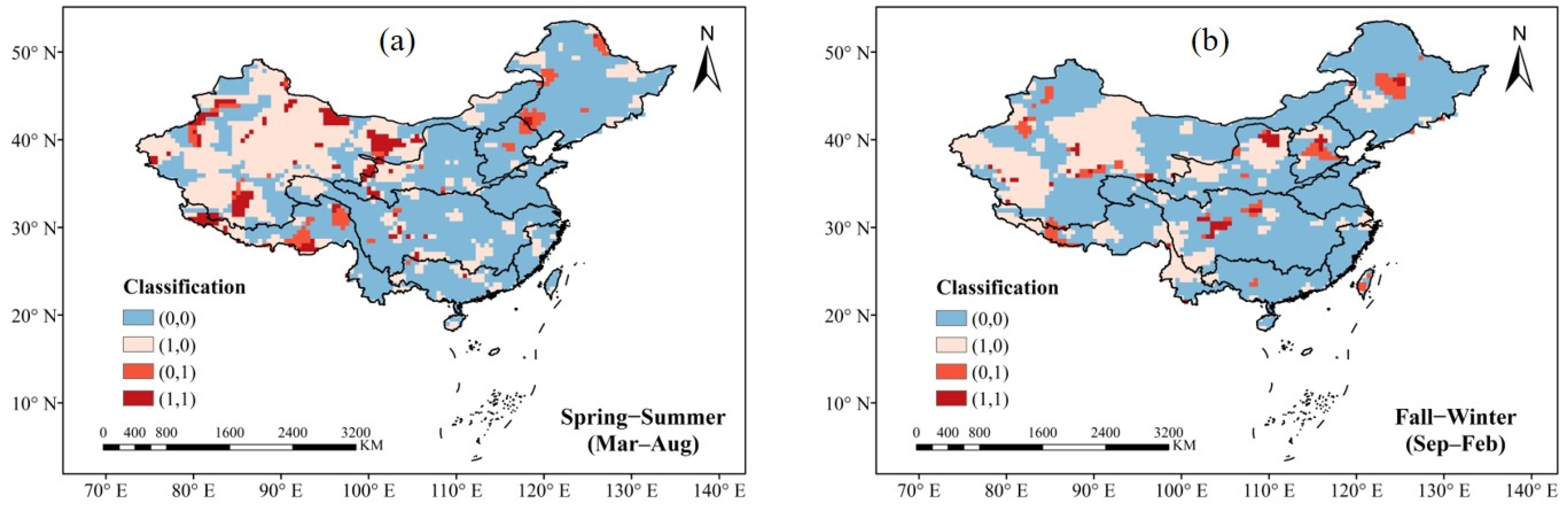
Drought warnings should focus on Northwest and Southwest China; the former and latter were under-estimated in the spring–summer and the fall–winter seasons, respectively, under the current stationary drought index assessment system.

In conclusion, this study provides support for drought assessment and early warning systems that consider non-stationarity under climate change.

References

1. Mishra, A.K.; Singh, V.P. A review of drought concepts. J. Hydrol. 2010, 391, 202–216. [Google Scholar] [CrossRef]
2. Kogan, F.N. Global drought watch from space. Bull. Am. Meteorol. Soc. 1997, 78, 621–636. [Google Scholar] [CrossRef]
3. Zhang, L.; Zhou, T. Drought over East Asia: A review. J. Clim. 2015, 28, 3375–3399. [Google Scholar] [CrossRef]
4. Yang, J.; Gong, D.; Wang, W.; Hu, M.; Mao, R. Extreme drought event of 2009/2010 over southwestern China. Meteorol. Atmos. Phys. 2012, 115, 173–184. [Google Scholar] [CrossRef]
5. Guo, E.; Liu, X.; Zhang, J.; Wang, Y.; Wang, C.; Wang, R.; Li, D. Assessing spatiotemporal variation of drought and its impact on maize yield in Northeast China. J. Hydrol. 2017, 553, 231–247. [Google Scholar] [CrossRef]
6. Das, S.; Das, J.; Umamahesh, N.V. Nonstationary modeling of meteorological droughts: Application to a region in India. J. Hydrol. Eng. 2021, 26, 05020048. [Google Scholar] [CrossRef]
7. Soľáková, T.; De Michele, C.; Vezzoli, R. Comparison between parametric and nonparametric approaches for the calculation of two drought indices: SPI and SSI. J. Hydrol. Eng. 2014, 19, 04014010. [Google Scholar] [CrossRef]
8. Heim, R.R., Jr. A review of twentieth-century drought indices used in the United States. Bull. Am. Meteorol. Soc. 2002, 8, 1149–1166. [Google Scholar] [CrossRef]
9. Wilhite, D.A.; Glantz, M.H. Understanding: The drought phenomenon: The role of definitions. Water Int. 1985, 10, 111–120. [Google Scholar] [CrossRef]
10. Dracup, J.A.; Lee, K.S.; Paulson, E.G., Jr. On the definition of droughts. Water Resour. Res. 1980, 16, 297–302. [Google Scholar] [CrossRef]
11. Huang, S.; Li, P.; Huang, Q.; Leng, G.; Hou, B.; Ma, L. The propagation from meteorological to hydrological drought and its potential influence factors. J. Hydrol. 2017, 547, 184–195. [Google Scholar] [CrossRef]
12. Ding, Y.; Xu, J.; Wang, X.; Cai, H.; Zhou, Z.; Sun, Y.; Shi, H. Propagation of meteorological to hydrological drought for different climate regions in China. J. Environ. Manag. 2021, 283, 111980. [Google Scholar] [CrossRef]
13. Van Loon, A.F. Hydrological drought explained. Wiley Interdiscip. Rev. Water 2015, 2, 359–392. [Google Scholar] [CrossRef]
14. Mannocchi, F.; Todisco, F.; Vergni, L. Agricultural drought: Indices, definition and analysis. In International Symposium on Basis of Civilization—Water Science; International Association of Hydrological Science: Rome, Italy, 2004. [Google Scholar]
15. Edwards, B.; Gray, M.; Hunter, B. The social and economic impacts of drought. Aust. J. Soc. Issues 2019, 54, 22–31. [Google Scholar] [CrossRef]
16. Palmer, W.C. Meteorological Drought; US Department of Commerce, Weather Bureau: Silver Sprin, MD, USA, 1965; Volume 30.
17. McKee, T.B.; Doesken, N.J.; Kleist, J. The relationship of drought frequency and duration to time scales. In Proceedings of the 8th Conference on Applied Climatology, Anaheim, CA, USA, 17–22 January 1993; Volume 17, pp. 179–183. [Google Scholar]
18. Vicente-Serrano, S.M.; Beguería, S.; López-Moreno, J.I. A multiscalar drought index sensitive to global warming: The standardized precipitation evapotranspiration index. J. Clim. 2010, 23, 1696–1718. [Google Scholar] [CrossRef]
19. Zarch, M.A.A.; Sivakumar, B.; Sharma, A. Droughts in a warming climate: A global assessment of Standardized Precipitation Index (SPI) and Reconnaissance Drought Index (RDI). J. Hydrol. 2015, 526, 183–195. [Google Scholar] [CrossRef]
20. Wu, J.; Miao, C.; Tang, X.; Duan, Q.; He, X. A nonparametric standardized runoff index for characterizing hydrological drought on the Loess Plateau, China. Glob. Planet. Chang. 2018, 161, 53–65. [Google Scholar] [CrossRef]
21. Shafer, B.A.; Dezman, L.E. Development of surface water supply index (SWSI) to assess the severity of drought condition in snowpack runoff areas. In Proceedings of the Western Snow Conference, Reno, Nevada, 19–23 April 1982. [Google Scholar]
22. Palmer, W.C. Keeping track of crop moisture conditions, nationwide: The new crop moisture index. Weatherwise 1968, 21, 156–161. [Google Scholar] [CrossRef]
23. Sohrabi, M.M.; Ryu, J.H.; Abatzoglou, J.; Tracy, J. Development of soil moisture drought index to characterize droughts. J. Hydrol. Eng. 2015, 20, 04015025. [Google Scholar] [CrossRef]
24. Bushra, N.; Rohli, R.V.; Lam, N.S.N.; Zou, L.; Mostafiz, R.B.; Mihunov, V. The relationship between the normalized difference vegetation index and drought indices in the South Central United States. Nat. Hazards 2019, 96, 791–808. [Google Scholar] [CrossRef]
25. Guo, X.; Gao, W.; Richard, P.; Lu, Y.; Zheng, Y.; Pietroniro, E. Canadian prairie drought assessment through MODIS vegetation indices. In Remote Sensing and Modeling of Ecosystems for Sustainability; SPIE: Bellingham, WA, USA, 2004; Volume 5544, pp. 149–158. [Google Scholar]
26. Yan, X.; Lin, M.; Chen, X.; Yao, H.; Liu, C.; Lin, B. A new method to restore the impact of land-use change on flood frequency based on the Hydrologic Engineering Center-Hydrologic Modelling System model. Land Degrad. Dev. 2020, 31, 1520–1532. [Google Scholar] [CrossRef]
27. Wang, M.; Jiang, S.; Ren, L.; Xu, C.; Wei, L.; Cui, H.; Yuan, F.; Liu, Y.; Yang, X. The development of a nonstationary standardised streamflow index using climate and reservoir indices as covariates. Water Resour. Manag. 2022, 36, 1377–1392. [Google Scholar] [CrossRef]
28. Zhang, T.; Su, X.; Feng, K. The development of a novel nonstationary meteorological and hydrological drought index using the climatic and anthropogenic indices as covariates. Sci. Total Environ. 2021, 786, 147385. [Google Scholar] [CrossRef]
29. Milly, P.C.; Betancourt, J.; Falkenmark, M.; Hirsch, R.M.; Kundzewicz, Z.W.; Lettenmaier, D.P.; Stouffer, R.J. Stationarity is dead: Whither water management? Science 2008, 319, 573–574. [Google Scholar] [CrossRef]
30. Rigby, R.A.; Stasinopoulos, D.M. Generalized additive models for location, scale and shape. J. R. Stat. Soc. C Appl. Stat. 2005, 54, 507–554. [Google Scholar] [CrossRef]
31. Song, Z.; Xia, J.; She, D.; Zhang, L.; Hu, C.; Zhao, L. The development of a Nonstationary Standardized Precipitation Index using climate covariates: A case study in the middle and lower reaches of Yangtze River Basin, China. J. Hydrol. 2020, 588, 125115. [Google Scholar] [CrossRef]
32. Sun, X.; Li, Z.; Tian, Q. Assessment of hydrological drought based on nonstationary runoff data. Hydrol. Res. 2020, 51, 894–910. [Google Scholar] [CrossRef]
33. Russo, S.; Dosio, A.; Sterl, A.; Barbosa, P.; Vogt, J. Projection of occurrence of extreme dry-wet years and seasons in Europe with stationary and nonstationary Standardized Precipitation Indices. J. Geophys. Res. Atmos. 2013, 118, 7628–7639. [Google Scholar] [CrossRef]
34. Shiau, J. Effects of gamma-distribution variations on SPI-Based stationary and nonstationary drought analyses. Water Resour. Manag. 2020, 34, 2081–2095. [Google Scholar] [CrossRef]
35. Wang, Y.; Li, J.; Feng, P.; Hu, R. A time-dependent drought index for non-stationary precipitation series. Water Resour. Manag. 2015, 29, 5631–5647. [Google Scholar] [CrossRef]
36. Ju, X.; Wang, Y.; Wang, D.; Singh, V.P.; Xu, P.; Wu, J.; Ma, T.; Liu, J.; Zhang, J. A time-varying drought identification and frequency analyzation method: A case study of Jinsha River Basin. J. Hydrol. 2021, 603, 126864. [Google Scholar] [CrossRef]
37. Zou, L.; Xia, J.; Ning, L.; She, D.; Zhan, C. Identification of hydrological drought in Eastern China using a time-dependent drought index. Water 2018, 10, 315. [Google Scholar] [CrossRef]
38. Kang, L.; Jiang, S. Bivariate frequency analysis of hydrological drought using a nonstationary standardized streamflow index in the Yangtze river. J. Hydrol. Eng. 2019, 24, 05018031. [Google Scholar] [CrossRef]
39. Bazrafshan, J.; Hejabi, S. A non-stationary reconnaissance drought index (NRDI) for drought monitoring in a changing climate. Water Resour. Manag. 2018, 32, 2611–2624. [Google Scholar] [CrossRef]
40. Li, J.Z.; Wang, Y.X.; Li, S.F.; Hu, R. A nonstationary standardized precipitation index incorporating climate indices as covariates. J. Geophys. Res. Atmos. 2015, 120, 12082–12095. [Google Scholar] [CrossRef]
41. Masanta, S.K.; Srinivas, V.V. Proposal and evaluation of nonstationary versions of SPEI and SDDI based on climate covariates for regional drought analysis. J. Hydrol. 2022, 610, 127808. [Google Scholar] [CrossRef]
42. Wang, Y.; Duan, L.; Liu, T.; Li, J.; Feng, P. A non-stationary standardized streamflow index for hydrological drought using climate and human-induced indices as covariates. Sci. Total Environ. 2020, 699, 134278. [Google Scholar] [CrossRef]
43. CPC Global Unified Gauge-Based Analysis of Daily Precipitation. Available online: https://psl.noaa.gov/data/gridded/data.cpc.globalprecip.html (accessed on 9 August 2020).
44. CPC Global Unified Temperature. Available online: https://psl.noaa.gov/data/gridded/data.cpc.globaltemp.html (accessed on 9 August 2020).
45. Mann, H.B. Nonparametric tests against trend. Econometrica 1945, 13, 245–259. [Google Scholar] [CrossRef]
46. Kendall, M.G. Rank Correlation Methods; Griffin Charles: London, UK, 1975; Volume 120. [Google Scholar]
47. Gu, X.; Zhang, Q.; Singh, V.P.; Shi, P. Nonstationarity in timing of extreme precipitation across China and impact of tropical cyclones. Glob. Planet. Chang. 2017, 149, 153–165. [Google Scholar] [CrossRef]
48. Oliveira, P.T.; Santos e Silva, C.M.; Lima, K.C. Climatology and trend analysis of extreme precipitation in subregions of Northeast Brazil. Theor. Appl. Climatol. 2017, 130, 77–90. [Google Scholar] [CrossRef]
49. Thornthwaite, C.W. An approach toward a rational classification of climate. Geogr. Rev. 1948, 38, 55–94. [Google Scholar] [CrossRef]
50. Yimer, E.A.; Van Schaeybroeck, B.; Van de Vyver, H.; Van Griensven, A. Evaluating probability distribution functions for the Standardized Precipitation Evapotranspiration Index over Ethiopia. Atmosphere 2022, 13, 364. [Google Scholar] [CrossRef]
51. Cole, T.J.; Green, P.J. Smoothing reference centile curves: The LMS method and penalized likelihood. Stat. Med. 1992, 11, 1305–1319. [Google Scholar] [CrossRef]
52. Rigby, R.A.; Stasinopoulos, D.M. A semi-parametric additive model for variance heterogeneity. Stat. Comput. 1996, 6, 57–65. [Google Scholar] [CrossRef]
53. Rigby, B.S.; Harley, R.G. The development of an advanced series compensator based on a single voltage source inverter. In Proceedings of the IEEE AFRICON′96, Stellenbosch, South Africa, 27 September 1996; pp. 215–220. [Google Scholar]
54. Akaike, H. Citation classic—A new look at the statistical-model identification. Curr. Contents/Eng. Technol. Appl. Sci. 1981, 51, 22. [Google Scholar]
55. Sun, J.; Ao, J. Changes in precipitation and extreme precipitation in a warming environment in China. Sci. Bull. 2013, 58, 1395–1401. [Google Scholar] [CrossRef]
56. Wu, Y.; Wu, S.; Wen, J.; Xu, M.; Tan, J. Changing characteristics of precipitation in China during 1960–2012. Int. J. Climatol. 2016, 36, 1387–1402. [Google Scholar] [CrossRef]
57. Mavromatis, T. Drought index evaluation for assessing future wheat production in Greece. Int. J. Climatol. 2007, 27, 911–924. [Google Scholar] [CrossRef]
58. Chen, H.; Sun, J. Changes in drought characteristics over China using the standardized precipitation evapotranspiration index. J. Clim. 2015, 28, 5430–5447. [Google Scholar] [CrossRef]
Figure 1. Study area. The study area was divided according to nine river basins in China; the Songliao River Basin (SRB), the Haihe River Basin (HRB1), the Huaihe River Basin (HRB2), the Yellow River Basin (YRB1), the Yangtze River Basin (YRB2), the Southeast River Basin (SRB1), the Southwest River Basin (SRB2), the Pearl River Basin (PRB), and the Continental River Basin (CRB), respectively.
Applsci 12 08479 g001
Figure 2. Spatiotemporal distribution of the long-term trends of P, PET, and D series. Black dots indicate confidence levels of 95% or more.
Applsci 12 08479 g002
Figure 3. Performances of nonstationary and stationary models under AIC assessment. (a) and (b) are the stationary and nonstationary models, respectively; (1) and (2) are the AIC values for the seventh and fifth-months, respectively.
Applsci 12 08479 g003
Figure 4. Changes in location and scale (μ, σ) parameters for the nonstationary model. 1 indicates a trend that passes the 95% confidence test, and 0 indicates either no trend or one that does not pass the 95% confidence level. (a) distribution parameter change class in spring–summer season; (b) distribution parameter change class in fall–winter season.
Applsci 12 08479 g004
Figure 5. Percentage of differences in drought characteristics under NSPEI and SPEI. (a_1) shows the duration in the spring–summer seasons; (a_2) shows the severity in the spring–summer seasons; (b_1) shows the duration in the fall–winter seasons; (b_2) shows the severity in the fall–winter seasons.
Applsci 12 08479 g005
Figure 6. Probability density of duration estimated by SPEI and NSPEI in the nine river basins of China under different classifications of (μ, σ) changes in the spring–summer season.
Applsci 12 08479 g006
Figure 7. Probability density of severity estimated by SPEI and NSPEI in the nine river basins of China under different classifications of (μ, σ) changes in the spring–summer season.
Applsci 12 08479 g007
Figure 8. Probability density of duration estimated by SPEI and NSPEI in the nine river basins of China under different classifications of (μ, σ) changes in the fall–winter season.
Applsci 12 08479 g008
Figure 9. Probability density of severity estimated by SPEI and NSPEI in the nine river basins of China under different classifications of (μ, σ) changes in the fall–winter season.
Applsci 12 08479 g009