A Differential Subgrid Stress Model and Its Assessment in Large Eddy Simulations of Non-Premixed Turbulent Combustion

Abstract

We present a new subgrid stress model for the large eddy simulation of turbulent flows based on the solution of transport equations for stress tensor components. The model was a priori term-by-term calibrated against an open DNS database on forced isotropic turbulence (Johns Hopkins University database). After that, it was applied in a large eddy simulation of non-premixed turbulent combustion. To demonstrate the impact of the new subgrid stress model on scalar fields, we excluded the backward effect of heat release on the subgrid stresses, considering an isothermal reaction (i.e., diluted mixture; the density variations associated with chemical heat release can be neglected) and a Burke–Schumann reaction sheet approximation. A periodic box filled with a homogeneous turbulent velocity field and a three-layer top-hat mixture fraction field was studied. Four simulations were performed in which a fixed model for mixture fraction and its variance was combined with either the proposed subgrid stress model or one of the standard models, including Smagorinsky, dynamic Smagorinsky and WALE. Qualitatively correct backscatter was observed in a simulation with the new model. The differences in the statistics of the mixture fraction and reactive component fields caused by the new subgrid stress model were analyzed and discussed. The importance of using an advanced subgrid stress model was highlighted.

1. Introduction

Presently, almost all large eddy simulations (LESs) are carried out with the use of either algebraic or differential subgrid viscosity models [1]. Non-negative subgrid viscosity, ${\nu }_{sgs}$, prevents these models from capturing the regions of “reverse” energy flux from subgrid scales to resolved ones, or backscatter, observed experimentally [2] and numerically [3]. A dynamic procedure alleviates this problem by allowing negative ${\nu }_{sgs}$ values [4]. However, this approach suffers from numerical instability, and a common way to stabilize a dynamic model is to introduce ${\nu }_{sgs}$ clipping [5] or spatial averaging [6]. A more theoretically justified way to address the issue of backscatter may be to employ a differential subgrid stress model (DSM) in which a differential equation is solved for each component of a subgrid stress tensor. In DSM, the principal axes of stress and strain tensors as well as their eigenvalues are decoupled. This allows the simulation of inefficient and even locally reversed energy cascades, as recently studied by analyzing DNS data [3].

Although there is evidence that the correct choice of subgrid model may be crucial for a successful LES [7,8], there are still few papers on this topic [9,10,11,12,13]. Pioneering research was published by J.W. Deardorff [9], who formulated the first DSM in 1973 and conducted atmospheric turbulence simulations on a 40 × 40 × 20 gird, demonstrating improved results compared with eddy viscosity models. After more than two decades, C. Fureby et al. published an updated version of a DSM [10] and discussed its potential benefits. Since the 2010s, several papers have been published [11,12,13] on hybrid RANS/LES models which combine a differential Reynolds stress model near a wall with a DSM built on the same basis. Thus, research on DSMs is presently entering its active phase.

Subgrid models also determine the scalar dissipation field and the smallest resolved eddy structure. Both factors have an essential influence on the characteristics of non-premixed turbulent flames, controlled by mixing fuel with an oxidizer. Thus, an advanced subgrid stress model can also improve the predictions of turbulent diffusion combustion.

The current paper contributes to the development of a DSM. A systematic approach is presented to choose appropriate closures and calibrate their coefficients using an open DNS database. The resulting model is compared with the classical Smagorinsky model [14], its dynamic version [4] and a popular WALE model [15] in large eddy simulations of turbulent diffusion combustion. To simplify the task and exclude the backward influence of combustion on the turbulence, a case of so-called isothermal combustion [16] was used. Additional simplifications include consideration of a one-stage unidirectional reaction, proceeding at an infinite speed (Burke–Schumann reaction sheet approximation [17]). The average rates of chemical reactions were determined using the classical non-premixed flamelet approach [18]. Estimates of the differences in the statistics of the mixture fraction fields were obtained, analyzed and discussed.

The structure of the paper is as follows. In Section 2, closures for the terms in the subgrid stress tensor equation are proposed, and coefficient calibration is discussed and performed. In Section 3, an LES of homogeneous turbulence in a periodic box is presented. A three-layer initial field of mixture fraction, corresponding to a fuel layer placed between two oxidizer layers, is considered. Mixture composition fields, developing due to isothermal combustion, are obtained at each time moment by processing the instantaneous fields of mixture fraction and dispersion. The new DSM is compared to the standard subgrid viscosity models. In Section 4, the results are discussed, followed by our conclusions.

2. Subgrid Stress Tensor Equation Closure and Calibration

2.1. Subgrid Stress Tensor Equation

We base this research on the incompressible Navier–Stokes equations, as follows:

$$\frac{\partial u_i}{\partial x_i}=0,$$

(1)

$$\frac{\partial u_i}{\partial t}+u_k\frac{\partial u_i}{\partial x_k}=-\frac{1}{\rho }\frac{\partial p}{\partial x_i}+\nu \frac{{\partial }^2{u}_i}{\partial x_k\partial x_k}.$$

(2)

Summation over repeated indices is implied.

After spatial filtering denoted by an overbar, an additional term called subgrid stress tensor appears in the following momentum equation:

$$\frac{\partial {\overline{u}}_i}{\partial t}+{\overline{u}}_k\frac{\partial {\overline{u}}_i}{\partial x_k}+\frac{\partial \overline{u_i^{\prime }{u}_k^{\prime }}}{\partial x_k}=-\frac{1}{\rho }\frac{\partial \overline{p}}{\partial x_i}+\nu \frac{{\partial }^2{\overline{u}}_i}{\partial x_k\partial x_k}.$$

Hereinafter, cumulants [19], or central moments [20], are used to abbreviate the following notation:

$$\overline{a^{\prime }{b}^{\prime }}=\overline{ab}-\overline{a}\overline{b}, \overline{a^{\prime }{b}^{\prime }{c}^{\prime }}=\overline{abc}-\overline{a}\overline{b\prime c\prime }-\overline{b}\overline{c\prime a\prime }-\overline{c}\overline{a\prime b\prime }-\overline{a}\overline{b}\overline{c}.$$

By combining (1) and (2) and applying a filtering operator, one can obtain the following differential equation for the subgrid stress tensor:

$$\begin{gathered} \frac{\partial \overline{u_i^{\text{'}}{u}_j^{\text{'}}}}{\partial t}+\frac{\partial }{\partial x_k}\left[\overline{u_i^{\text{'}}{u}_j^{\text{'}}} {\overline{u}}_k+\overline{u_i^{\text{'}}{u}_j^{\text{'}}{u}_k^{\text{'}}}+\frac{1}{\rho }\left(\overline{p^{\prime }{u}_i^{\text{'}}}{\delta }_{jk}+\overline{p^{\prime }{u}_j^{\text{'}}}{\delta }_{ik}\right)-\nu \frac{\partial \overline{u_i^{\text{'}}{u}_j^{\text{'}}}}{\partial x_k}\right] \\ =-\overline{u_i^{\text{'}}{u}_k^{\text{'}}}\frac{\partial {\overline{u}}_j}{\partial x_k}-\overline{u_j^{\text{'}}{u}_k^{\text{'}}}\frac{\partial {\overline{u}}_i}{\partial x_k}+\frac{1}{\rho }\overline{p^{\prime }\left(\frac{\partial u_i^{\text{'}}}{\partial x_j}+\frac{\partial u_j^{\text{'}}}{\partial x_i}\right)}-2\nu \overline{\frac{\partial u_i^{\text{'}}}{\partial x_k}\frac{\partial u_j^{\text{'}}}{\partial x_k}} \end{gathered}$$

(3)

The terms in this equation can be interpreted as follows. On the LHS, under the divergence symbol, there are advection by a resolved flow field, turbulent transport due to subgrid-scale velocity fluctuations, turbulent transport due to subgrid-scale pressure fluctuations and molecular transport, respectively. On the RHS, the first two terms represent the subgrid stress tensor production. This is followed by a pressure–strain correlation which acts as redistribution between energy components in the principal frame of $\overline{u_i^{\prime }{u}_j^{\prime }}$. The last term in (3) represents the subgrid stress viscous dissipation. Turbulent transport terms, the pressure–strain correlation and the dissipation tensor require closure models.

2.2. Closure

We are not aiming to construct the best possible closure model for unclosed terms in (3). Our goal is rather to optimize the coefficients of some typical form of closures based on DNS data. According to this, we use locally isotropic assumption, leading to

$$2\nu \overline{\frac{\partial u_i^{\prime }}{\partial x_k}\frac{\partial u_j^{\prime }}{\partial x_k}}=\frac{2}{3}\epsilon {\delta }_{ij}, \epsilon =\nu \overline{\frac{\partial u_i^{\prime }}{\partial x_k}\frac{\partial u_j^{\prime }}{\partial x_k}},$$

where ε is the subgrid kinetic energy dissipation rate. It is natural to express ε in terms of subgrid kinetic energy, $k=\overline{u_i^{\prime }{u}_i^{\prime }}/2$, and characteristic filter size, Δ, as follows:

$$\epsilon =C_E\frac{k^{3/2}}{\mathsf{\Delta }}.$$

(4)

The simplest model assumes $C_E=const$; however, due to the importance of accurate representation of the dissipation process, we will consider a dependence of $C_E$ on invariants of subgrid stress anisotropy tensor $a=\left(a_{ij}\right)$:

$$C_E=C_E^{\left(0\right)}+C_E^{\left(1\right)}{A}_2+C_E^{\left(2\right)}{A}_3.$$

(5)

Here, $a_{ij}$, $A_2$ and $A_3$ are defined as

$$a_{ij}=\frac{\overline{u_i^{\prime }{u}_j^{\prime }}}{k}-\frac{2}{3}{\delta }_{ij}, A_2=a_{ij}{a}_{ji}, A_3=a_{ij}{a}_{jk}{a}_{ki}.$$

(6)

Equation (5) can be considered as Taylor expansion of $C_E$ in the corresponding variables.

The pressure–strain correlation tensor, denoted hereinafter as $\Phi =\left({\mathsf{\Phi }}_{ij}\right)$, is usually expanded in powers of $a$. The most general form of linear model for $\Phi$ is the following [21]:

$$\Phi =-C_{\mathsf{\Phi }1}a\epsilon +k\left[C_{\mathsf{\Phi }2}S+C_{\mathsf{\Phi }3}\left(aS+Sa-\frac{2}{3}\mathrm{tr}\left(aS\right)I\right)+C_{\mathsf{\Phi }4}\left(\Omega a-a\Omega \right)\right],$$

(7)

with tensor multiplication obeying the matrix rule, ${\left(AB\right)}_{ij}=A_{ik}{B}_{kj}$. Here, $I=\left({\delta }_{ij}\right)$ is a unity tensor; $S$ and $\Omega$ are resolved strain rate and rotation tensors, respectively,

$$S_{ij}=\frac{1}{2}\left(\frac{\partial {\overline{u}}_i}{\partial x_j}+\frac{\partial {\overline{u}}_j}{\partial x_i}\right), {\mathsf{\Omega }}_{ij}=\frac{1}{2}\left(\frac{\partial {\overline{u}}_i}{\partial x_j}-\frac{\partial {\overline{u}}_j}{\partial x_i}\right).$$

Again, the simplest model assumes $C_{\mathsf{\Phi }1},\dots ,C_{\mathsf{\Phi }4}$ to be constants, but an inclusion of dependence on $A_2$ and $A_3$ may be considered as means to improve the model.

For the triple-velocity correlation, we use a gradient model modified by means of resolved velocity gradients, the presence of which follows from exact the equation for $\overline{u_i^{\prime }{u}_j^{\prime }{u}_k^{\prime }}$ [22], as follows:

$$\overline{u_i^{\prime }{u}_j^{\prime }{u}_k^{\prime }}={\displaystyle \sum }_{\left\{i\to j\to k\right\}}\left[-k^{1/2}\mathsf{\Delta }\left(C_{T1}{\delta }_{kl}+C_{T2}{a}_{kl}\right)+C_{T3}{\mathsf{\Delta }}^2\frac{\partial {\overline{u}}_k}{\partial x_l}\right]\frac{\partial \overline{u_i^{\prime }{u}_j^{\prime }}}{\partial x_l}.$$

(8)

Summation is performed over cyclic permutations of the i, j and k indices:

$${\displaystyle \sum }_{\left\{i\to j\to k\right\}}{A}_{ijk}=A_{ijk}+A_{jki}+A_{kij}.$$

The coefficients $C_{T1},C_{T2},C_{T3}$ can be either constants or functions of $A_2$ and $A_3$.

It remains to consider the pressure–velocity correlation. According to [23], one can approximate it by contracting the triple-velocity correlation tensor:

$$\frac{1}{\rho }\overline{p^{\prime }{u}_i^{\prime }}=-C_{PT}\overline{u_i^{\prime }{u}_m^{\prime }{u}_m^{\prime }}.$$

(9)

There is one empirical coefficient: $C_{PT}$.

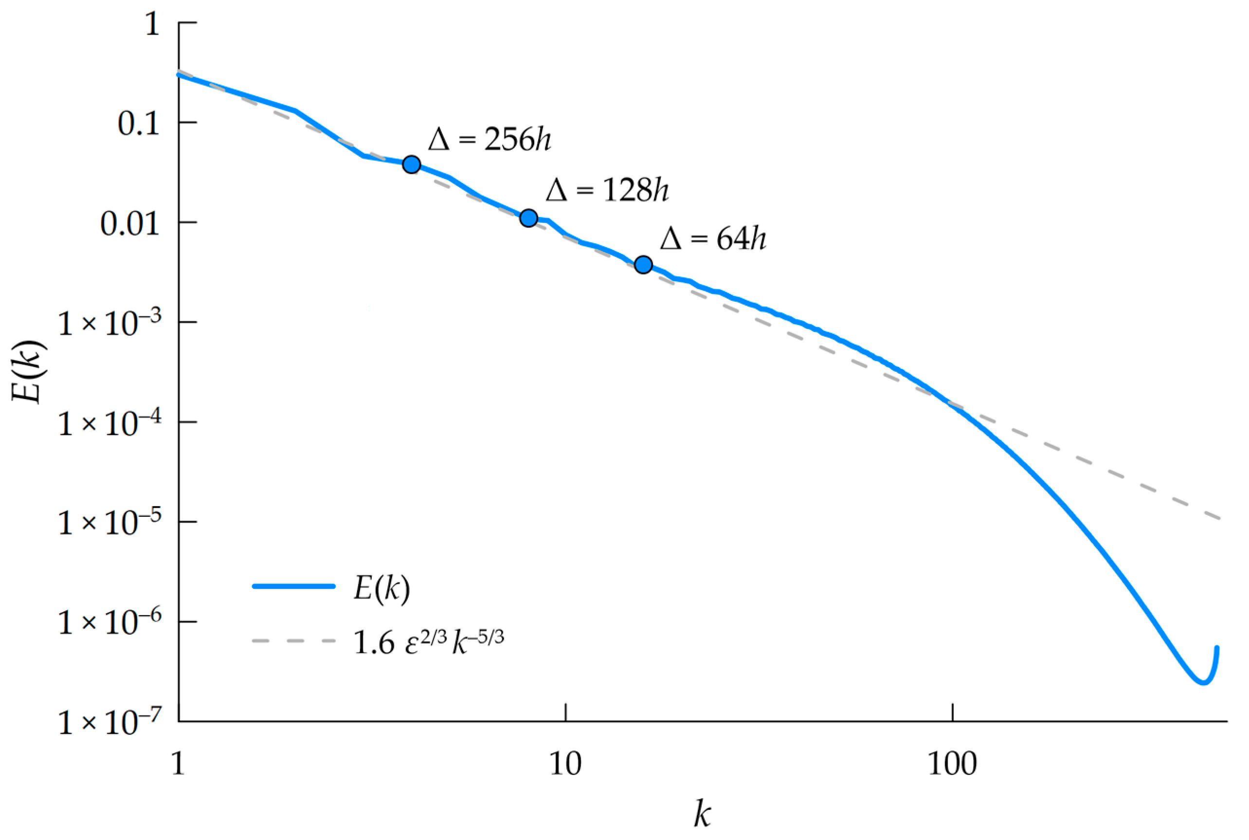
2.3. DNS Database and Filtering

To calibrate the coefficients in the formulated models, a DNS dataset that was representative of typical subgrid-scale turbulence was required. We used a computation of forced isotropic turbulence [24] from the Johns Hopkins Turbulence Database [25] for this purpose. This dataset was originally generated with a pseudo-spectral algorithm in a periodic domain of size $L\times L\times L$ with uniform grid of ${1024}^3$ points, $L=2\pi$. In this flow, the Reynolds number, with respect to the Taylor microscale, is equal to 433; the Kolmogorov microscale is equal to 0.46 h, where h is grid spacing, the integral length scale is equal to 0.217 L; the integral time scale is equal to 0.2 T, where T is simulation period after attaining a statistically steady state. All the numbers are nondimensional.

We extracted 11 snapshots separated by 0.1 T and filtered them using a box filter of different sizes, Δ. Three filter sizes were considered: $\mathsf{\Delta }=64 h$, $\mathsf{\Delta }=128 h$ and $\mathsf{\Delta }=256 h$. In Figure 1, their positions on a radial kinetic energy spectrum are shown. While $\mathsf{\Delta }=64 h$ is close to the bottom part of the inertial interval, two larger filters are significantly inside it, which corresponds to a correct LES.

To process the filtered data effectively, we extracted an “LES grid” from each filtered field with the spatial step $h_{LES}=\mathsf{\Delta }/4$. The derivatives of filtered fields on the RHS of (7) and (8) were calculated by a central difference formula on LES grids, for example:

$${\left(\frac{\partial \overline{u}}{\partial x}\right)}_{\alpha ,\beta ,\gamma }\approx \frac{{\overline{u}}_{\alpha +1,\beta ,\gamma }-{\overline{u}}_{\alpha -1,\beta ,\gamma }}{2h_{LES}}.$$

(10)

A comparison of spatially averaged, scale-to-scale energy flux, $P=-\overline{u_i^{\prime }{u}_j^{\prime }} S_{ij}$, calculated first using finite differences (10) and after that employing “exact” values of $\partial {\overline{u}}_i/\partial x_j$, showed that the error induced by the finite spatial step was within 3%.

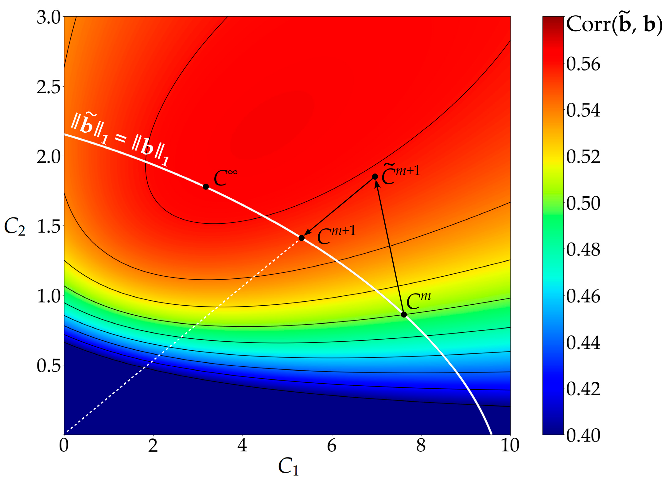
2.4. Calibration Method

In each of the closures in (4), (5), (7), (8) and (9), the empirical coefficients enter linearly. The naïve method of their calibration is to obtain coefficient values from an overdetermined linear equation system by the least squares method, with each equation corresponding to a single data point at a single time instance and a single tensor component. Suppose we have a one-dimensional data vector, $b$, formed in this way, and that its model is $\tilde{b}=C_1{a}_1+\dots +C_n{a}_n$. Here, $a_i$ and $b$ are exact filtered DNS data. Then, the least squares solution of overdetermined linear system is as follows:

$$C_1{a}_1+\dots +C_n{a}_n=b$$

which, with respect to $C_1,\dots ,C_n$, gives the coefficients which minimize the Euclidean distance $\parallel \tilde{b}-b{\parallel }_2$, where

$$\parallel x{\parallel }_p={\left({\displaystyle \sum }_i{\left|x_i\right|}^p\right)}^{1/p}.$$

The corresponding model $\tilde{b}$ can be interpreted as orthogonal projection of $b$ onto the linear span of $\left\{a_1,\dots ,a_n\right\}$. However, a drawback follows: if the “basis vectors” $a_1,\dots ,a_n$ are inadequate to represent the data vector $b$, the model vector $\tilde{b}$ will have significantly smaller norm than that of $b$. In our preliminary tests, for example, we were systematically obtaining the models for $\Phi$ in the form of (7), such that $\parallel \tilde{\Phi }{\parallel }_2/\parallel \Phi {\parallel }_2\approx 0.4\dots 0.5$.

Having faced this problem, we developed a calibration strategy, which is—to our knowledge—a new approach. Let us introduce a correlation coefficient between $\tilde{b}$ and $b$:

$$\mathrm{Corr}\left(\tilde{b}, b\right)=\frac{\left({\tilde{b}}_{\alpha }-‹{\tilde{b}}_{\alpha }›\right)\left(b_{\alpha }-‹b_{\alpha }›\right)}{\parallel \tilde{b}-‹\tilde{b}›{\parallel }_2 \parallel b-‹b›{\parallel }_2}$$

where angle brackets denote averaging over whole filtered dataset. Then, we can perform an iteration process. Denoting the coefficient approximation at the m^th iteration by $C_1^m,\dots ,C_n^m$, at the first step, we update their values by moving along the correlation coefficient gradient, as follows:

$${\tilde{C}}_i^{m+1}=C_i^m+K\frac{\partial \mathrm{Corr}\left(\tilde{b}, b\right)}{\partial C_i},$$

(11)

choosing the constant K to empirically maximize the convergence rate by maintaining the stability of the process (typically, K ranges from 0.5 to 10). In (11), we calculate the correlation coefficient derivative on the RHS by the following central difference formula:

$$\frac{\partial \mathrm{Corr}\left(\tilde{b}, b\right)}{\partial C_i}\approx \frac{\mathrm{Corr}\left(\dots +(C_i+\mathsf{\Delta }C\right)a_i+\dots , b)-\mathrm{Corr}\left(\dots +(C_i-\mathsf{\Delta }C\right)a_i+\dots , b)}{2\mathsf{\Delta }C}$$

with coefficient increment, $\mathsf{\Delta }C$, equal to ${10}^{-4}$. At the second step, we multiply the new coefficients by the norm ratio, $C_i^{m+1}=N{\tilde{C}}_i^{m+1}$, where $N=\parallel b{\parallel }_1/\parallel {\tilde{C}}_1^{m+1}{a}_1+\dots +{\tilde{C}}_n^{m+1}{a}_n{\parallel }_1$, to ensure the correct norm of the model. Here, we prefer the $L_1$ norm to avoid giving large weights to large data components. This procedure is repeated until the coefficients converge to a stationary state.

The idea of the method is visualized in Figure 2. A correlation coefficient contour is depicted as a function of two model coefficients, $C_1$ and $C_2$. The white solid line corresponds to pairs $C=\left\{C_1,C_2\right\}$, which yield a correct model norm, $\parallel \tilde{b}{\parallel }_1=\parallel b{\parallel }_1$. Let the coefficients at the mth iteration be at the $C^m$ point on the plot. The point, after moving along the correlation coefficient gradient, is denoted as ${\tilde{C}}^{m+1}$. Re-normalization corresponds to returning to the white solid line along the white dashed line (passing through the coordinate frame origin), so the new coefficients are $C^{m+1}$. The iterations converge to point $C^{\infty }$ on the plot, where the coefficient correlation is maximized, while the model norm is correct. To avoid falling to a local maximum, different initial conditions should be considered; however, all our tests revealed unique solutions independently of widely varied initial coefficient sets.

Finally, it is worth noting that, to avoid programming errors, the presented method was implemented independently by two authors. The identity of the results was verified.

2.5. Calibration Results

At the first step, we calibrated the dissipation rate model of the form (4) and (5). In

Table 1. Coefficients in the dissipation rate model (4) and (5).

$\mathrm{Filter} \mathrm{Size}, \Delta /h$	$C_E^{\left(0\right)}$	$C_E^{\left(1\right)}$	$C_E^{\left(2\right)}$	Correlation Coefficient
64	0.823	–1.308	1.848	0.861
128	0.804	–1.380	2.103	0.808
256	0.783	–1.421	2.305	0.717

, the calibrated coefficients are presented for different filter sizes together with their correlation coefficients.

The model correlates well with an exact $\epsilon$ field, yielding $\mathrm{Corr}$ of about 0.71–0.86. After averaging the coefficient values for different filter sizes and keeping two decimal digits, we propose the following dissipation model for use:

$$\begin{gathered} \epsilon =\max \left\{C_E^{\left(0\right)}+C_E^{\left(1\right)}{A}_2+C_E^{\left(2\right)}{A}_3, C_E^{lim}\right\}\frac{k^{3/2}}{\mathsf{\Delta }}, \\ {C}_E^{\left(0\right)}=0.8, C_E^{\left(1\right)}=-1.4, C_E^{\left(2\right)}=2.1, C_E^{lim}=0.21. \end{gathered}$$

(12)

Note that the inclusion of $A_2$ and $A_3$ is justified because the correlation coefficient of a constant coefficient model (with only $C_E^{\left(0\right)}$ non-zero) is approximately 0.11 lower. The maximum function is introduced to avoid possible undershoots of the dissipation rate in strongly anisotropic flow regions. We selected the value of $C_E^{lim}$ by referring to the probability density function of “exact” $C_E=\epsilon \mathsf{\Delta }/k^{3/2}$ distribution, as calculated from DNS data (see Figure 3). $C_E$ values lower than $C_E^{lim}=0.21$ are observed, with less than 1% probability.

At the second step, we investigated the constant coefficient model (7). The results are shown in

Table 2. Coefficients in the constant coefficient model (7).

$\mathbf{Filter} \mathbf{Size}, \mathsf{\Delta }/\mathit{h}$	${\mathit{C}}_{\mathsf{\Phi }1}$	${\mathit{C}}_{\mathsf{\Phi }2}$	${\mathit{C}}_{\mathsf{\Phi }3}$	${\mathit{C}}_{\mathsf{\Phi }4}$	Correlation Coefficient
64	2.020	1.364	0.449	0.791	0.590
128	1.850	1.283	0.384	0.681	0.664
256	1.630	1.222	0.324	0.587	0.747

.

Averaged coefficient values are $C_{\mathsf{\Phi }1}=1.8$, $C_{\mathsf{\Phi }2}=1.3$, $C_{\mathsf{\Phi }3}=0.39$ and $C_{\mathsf{\Phi }4}=0.69$. Unfortunately, the preliminary simulations using this model showed that it is unstable due to the value of $C_{\mathsf{\Phi }2}$ being too high. Our attempt to introduce the dependence of $C_{\mathsf{\Phi }1},\dots ,C_{\mathsf{\Phi }4}$ on $A_2$ and $A_3$ did not help. The model remained unstable, while its correlation coefficient increased only by 0.2%. After a series of attempts, we found a workable solution, which was to replace the $C_{\mathsf{\Phi }2}kS$ term in the model with the following:

$$\begin{gathered} C_{\mathsf{\Phi }2}^{\left(0\right)}kS+C_{\mathsf{\Phi }2}^{\left(1\right)}\sqrt{k}\mathsf{\Delta }\left(S\Omega -\Omega S\right)+C_{\mathsf{\Phi }2}^{\left(2\right)}\sqrt{k}\mathsf{\Delta }\left({\Omega }^2-\frac{1}{3}\mathrm{tr}\left({\Omega }^2\right)I\right) \\ +C_{\mathsf{\Phi }2}^{\left(3\right)}{\mathsf{\Delta }}^2\left(S\Omega \Omega +\Omega \Omega S-\frac{2}{3}\mathrm{tr}\left(S\Omega \Omega \right)I-\mathrm{tr}\left({\Omega }^2\right)S\right). \end{gathered}$$

(13)

The introduced nonlinear combinations of $S$ and $\Omega$ are widely used in the framework of EARSM [26]. The values of model coefficients obtained during the calibration are collected in

Table 3. Coefficients in the extended model (7), (13).

$\mathbf{Filter} \mathbf{Size}, \mathbf{\Delta }/\mathit{h}$	${\mathit{C}}_{\mathsf{\Phi }1}$	${\mathit{C}}_{\mathsf{\Phi }2}^{\left(0\right)}$	${\mathit{C}}_{\mathsf{\Phi }2}^{\left(1\right)}$	${\mathit{C}}_{\mathsf{\Phi }2}^{\left(2\right)}$	${\mathit{C}}_{\mathsf{\Phi }2}^{\left(3\right)}$	${\mathit{C}}_{\mathsf{\Phi }3}$	${\mathit{C}}_{\mathsf{\Phi }4}$	Correlation Coefficient
64	3.305	1.060	–0.134	–0.044	–0.269	0.356	1.335	0.604
128	3.046	1.030	–0.137	–0.061	–0.233	0.359	1.202	0.684
256	2.740	1.029	–0.137	–0.069	–0.191	0.313	1.014	0.760

.

Compared with the constant coefficient model, the correlation coefficient increased, on average, by 1%; however, the extended model turned out to produce stable solutions.

After averaging the data in Table 3, we formulated the following model:

$$\begin{gathered} \Phi =-C_{\mathsf{\Phi }1}a\epsilon +C_{\mathsf{\Phi }2}^{\left(0\right)}kS+C_{\mathsf{\Phi }2}^{\left(1\right)}\sqrt{k}\mathsf{\Delta }\left(S\Omega -\Omega S\right)+C_{\mathsf{\Phi }2}^{\left(2\right)}\sqrt{k}\mathsf{\Delta }\left({\Omega }^2-\frac{1}{3}\mathrm{tr}\left({\Omega }^2\right)I\right) \\ +C_{\mathsf{\Phi }2}^{\left(3\right)}{\mathsf{\Delta }}^2\left(S\Omega \Omega +\Omega \Omega S-\frac{2}{3}\mathrm{tr}\left(S\Omega \Omega \right)I-\mathrm{tr}\left({\Omega }^2\right)S\right)+C_{\mathsf{\Phi }3}k\left(aS+Sa-\frac{2}{3}\mathrm{tr}\left(aS\right)I\right)+C_{\mathsf{\Phi }4}k\left(\Omega a-a\Omega \right), \\ {C}_{\mathsf{\Phi }1}=3.0, C_{\mathsf{\Phi }2}^{\left(0\right)}=1.04, C_{\mathsf{\Phi }2}^{\left(1\right)}=-0.136, C_{\mathsf{\Phi }2}^{\left(2\right)}=-0.058, C_{\mathsf{\Phi }2}^{\left(3\right)}=-0.23, C_{\mathsf{\Phi }3}=0.34, C_{\mathsf{\Phi }4}=1.2. \end{gathered}$$

(14)

Consider now a triple-velocity correlation model (8). Again, starting with constant coefficients, $C_{T1},\dots ,C_{T3}$, we obtained the results collected in

Table 4. Coefficients in the constant coefficient model (8).

$\mathbf{Filter} \mathbf{Size}, \mathsf{\Delta }/\mathit{h}$	${\mathit{C}}_{\mathit{T}1}$	${\mathit{C}}_{\mathit{T}2}$	${\mathit{C}}_{\mathit{T}3}$	Correlation Coefficient
64	0.0178	0.0084	0.0615	0.869
128	0.0176	0.0042	0.0617	0.868
256	0.0207	0.0094	0.0665	0.844

. Interestingly, the corresponding term norms relate as follows:

$$\parallel C_{T1}{k}^{1/2}\mathsf{\Delta }{\displaystyle \sum }_{\left\{i\to j\to k\right\}}{\frac{\partial \overline{u_i^{\prime }{u}_j^{\prime }}}{\partial x_k}\parallel }_2:\parallel C_{T2}{k}^{1/2}\mathsf{\Delta }{\displaystyle \sum }_{\left\{i\to j\to k\right\}}{a}_{kl}{\frac{\partial \overline{u_i^{\prime }{u}_j^{\prime }}}{\partial x_l}\parallel }_2:\parallel C_{T3}{\mathsf{\Delta }}^2{\displaystyle \sum }_{\left\{i\to j\to k\right\}}\frac{\partial {\overline{u}}_k}{\partial x_l}{\frac{\partial \overline{u_i^{\prime }{u}_j^{\prime }}}{\partial x_l}\parallel }_2=6:1:53.$$

(15)

The second term in the model is clearly negligible, so we omitted it. The recalibration of the remaining coefficients is presented in

Table 5. Coefficients in the simplified model (8) without $C_{T2}$.

$\mathbf{Filter} \mathbf{Size}, \mathsf{\Delta }/\mathit{h}$	${\mathit{C}}_{\mathit{T}1}$	${\mathit{C}}_{\mathit{T}3}$	Correlation Coefficient
64	0.0185	0.0619	0.869
128	0.0179	0.0619	0.868
256	0.0211	0.0669	0.844

. Fortunately, the high correlation coefficient was not affected by the simplification.

An attempt to make transport coefficients dependent on $A_2$ and $A_3$ was unsuccessful, giving no significant improvements. The final model reads as follows:

$$\begin{gathered} \overline{u_i^{\prime }{u}_j^{\prime }{u}_k^{\prime }}={\displaystyle \sum }_{\left\{i\to j\to k\right\}}\begin{array}{c}\left[-C_{T1}{k}^{1/2}\mathsf{\Delta }{\delta }_{kl}+C_{T3}{\mathsf{\Delta }}^2\frac{\partial {\overline{u}}_k}{\partial x_l}\right]\frac{\partial \overline{u_i^{\prime }{u}_j^{\prime }}}{\partial x_l},\\ \end{array} \\ {C}_{T1}=0.019, C_{T3}=0.064. \end{gathered}$$

(16)

Making the model coefficients dependent on $A_2$ and $A_3$ allowed us to increase $\mathrm{Corr}$ only by 0.2–0.3%, which is impractical. Note that, according to (15), the leading term in the model (16) is the one containing the resolved velocity gradients. More traditional models, which do not contain explicit dependence on velocity gradients, perform significantly worse. Our tests show that a correlation coefficient for a model with only $C_{T1}$ non-zero has a $\mathrm{Corr}$ in the range 0.27–0.33, depending on $\mathsf{\Delta }$.

Finally, the optimal value of $C_{PT}$ in the pressure velocity correlation model given by (9) was found to be 0.482 for $\mathsf{\Delta }=64 h$, 0.422 for $\mathsf{\Delta }=128 h$ and 0.344 for $\mathsf{\Delta }=256 h$. The corresponding model,

$$\frac{1}{\rho }\overline{p^{\prime }{u}_i^{\prime }}=-C_{PT}\overline{u_i^{\prime }{u}_m^{\prime }{u}_m^{\prime }}, C_{PT}=0.42,$$

(17)

has correlation coefficient in the range 0.33–0.39, which is not promising. However, making $C_{PT}$ a function of local dimensionless parameters improved $\mathrm{Corr}$ by as little as 0.02, so we do not introduce such extensions to the final model.

Equations (12), (14), (16) and (17) form a closure of (3), which we propose in this paper.

2.6. Standard Subgrid Viscosity Models

In the current paper, we compare the performance of the proposed DSM with that of Smagorinsky model [14], dynamic Smagorinsky model [4] and WALE model [15], each extended with diagonal stress terms. These three models express the subgrid stress tensor as follows:

$$\overline{u_i^{\prime }{u}_j^{\prime }}=\frac{2}{3}k{\delta }_{ij}-2{\nu }_{sgs}{S}_{ij}.$$

(18)

In the Smagorinsky model, subgrid viscosity is defined as

$${\nu }_{sgs}={\left(C_{s}H\right)}^{2}S,$$

(19)

where $H$ is the computational grid spacing (equal to characteristic filter size $\mathsf{\Delta }$), $S=\sqrt{2S_{ij}{S}_{ij}}$ and $C_s$ is a constant coefficient. In dynamic Smagorinsky model, ${\nu }_{sgs}=C_{dyn}{H}^{2}S$, where

$$C_{dyn}=\min \left\{\max \left\{\frac{1}{\alpha }\frac{{ℒ}_{ml}{S}_{ml}}{H^2{\widetilde{SS}}_{kn}{S}_{kn}-{\alpha }^2{H}^2\tilde{S}{\tilde{S}}_{pq}{S}_{pq}}, C_{dyn}^{min}\right\}, C_{dyn}^{max}\right\},$$

(20)

$${ℒ}_{ij}=\widetilde{{\overline{u}}_i{\overline{u}}_j}-{\tilde{\overline{u}}}_i{\tilde{\overline{u}}}_j.$$

Tilda denotes averaging over a larger star-shaped filter of seven cells. Its size exceeds that of the original filter by a factor of $\alpha =\sqrt[3]{7}$. The coefficient is clipped on both sides to stabilize the model.

In the WALE model,

$${\nu }_{sgs}={\left(C_{W}H\right)}^2\frac{{\left({𝓈}_{ij}^d{𝓈}_{ij}^d\right)}^{3/2}}{{\left(S_{ij}{S}_{ij}\right)}^{5/2}+{\left({𝓈}_{ij}^d{𝓈}_{ij}^d\right)}^{5/4}},$$

where

$${𝓈}_{ij}^d=\frac{{\left(g^2\right)}_{ij}+{\left(g^2\right)}_{ji}}{2}-\frac{1}{3}{\left(g^2\right)}_{kk}{\delta }_{ij}, g_{ij}=\frac{\partial {\overline{u}}_i}{\partial x_j}, {\left(g^2\right)}_{ij}=g_{ik}{g}_{kj}$$

and $C_W$ is a constant coefficient. There are different approaches to determine the coefficient values [27,28]. In the next section, we find $C_s$, $C_{dyn}^{min}$, $C_{dyn}^{max}$ and $C_W$ from the requirement of obtaining the correct behavior of the energy spectrum in the inertial range.

In subgrid viscosity models, the subgrid kinetic energy can be evaluated by referring to the second invariant, $A_2$, of the anisotropy tensor, see Equation (6). According to the filtered DNS data, the volume-averaged $A_2$ value is $0.31\pm 0.04$ for the filter widths chosen in Section 2.3. From (18), $A_2$ is expressed as $2{\left({\nu }_{sgs}S/k\right)}^2$. Equating this to 0.31, we obtain

$$k={\left(\frac{2}{0.31}\right)}^{1/2}{\nu }_{sgs}S\approx 2.54{\nu }_{sgs}S.$$

We use this formula in the Smagorinsky and WALE models. In dynamic Smagorinsky model, we restrict the kinetic energy to non-negative values:

$$k=\max \left\{2.54{\nu }_{sgs}S, 0\right\}.$$

(21)

Finally, note that, when the DSM is employed, we approximate the subgrid viscosity which appears in the mixture fraction equations (see below) by the Smagorinsky formula (19) and determine $k$ according to its definition, $k=\overline{u_i^{\prime }{u}_i^{\prime }}/2$.

3. Large Eddy Simulations of Isothermal Combustion

3.1. Problem Statement and Numerical Setup

To study the subgrid model’s influence on the mixing and combustion process, we consider a three-layer top-hat mixture fraction field, transported by a homogeneous turbulent velocity field. Four simulations were performed using the new DSM, and the Smagorinsky, dynamic Smagorinsky and WALE models. In all cases, the flow corresponds to a non-premixed turbulent combustion regime without the backward effect of heat release. Since we use a compressible solver, we solve a compressible counterpart of (1) and (2), supplemented by an energy equation (molecular transport omitted due to formal $Re\to \infty$ limit):

$$\frac{\partial \overline{\rho }}{\partial t}+\frac{\partial \overline{\rho }{\overline{u}}_i}{\partial x_i}=0,$$

(22)

$$\frac{\partial \overline{\rho }{\overline{u}}_i}{\partial t}+\frac{\partial }{\partial x_k}\left[\overline{\rho }{\overline{u}}_i{\overline{u}}_k+\overline{p}{\delta }_{ik}+\overline{\rho }\overline{u_i^{\prime }{u}_k^{\prime }}\right]=0,$$

(23)

$$\frac{\partial \overline{\rho }\overline{E}}{\partial t}+\frac{\partial }{\partial x_k}\left[\overline{\rho }\overline{E}{\overline{u}}_k+\overline{p}{\overline{u}}_k+\overline{\rho }\overline{u_i^{\prime }{u}_k^{\prime }}{\overline{u}}_i+\frac{\overline{\rho }\overline{u_i^{\prime }{u}_i^{\prime }{u}_k^{\prime }}}{2}\right]=0.$$

(24)

This system is closed either by six equations obtained by introducing density into (3), or by algebraic relation (18). The expressions for total energy and state equation are as follows:

$$\overline{E}=\frac{{\overline{u}}_i{\overline{u}}_i}{2}+\frac{R\overline{T}}{\kappa -1}, \overline{p}=\overline{\rho }R\overline{T},$$

(25)

where $R\approx 287 \mathrm{J}/\left(\mathrm{kg}\cdot \mathrm{K}\right)$, $\kappa =1.4$. To minimize the compressibility effects, we make sure that the resolved field Mach number, $M={‹\left({\overline{u}}_i{\overline{u}}_i\right)}^{1/2}› /{\left(\kappa R‹T›\right)}^{1/2}$, stays less than 0.1 during the simulations (angle brackets denote averaging over the whole computational domain). Accordingly, we neglect the moments involving density fluctuations in (22)–(25).

The equation system is solved numerically using multiblock finite-volume in-house code zFlare [8] with a purely central second-order kinetic energy-preserving scheme [29] and an explicit three-step Heun time-integration method [30]. The time step, $\mathsf{\Delta }t$, satisfies the CFL condition, $\left({\overline{u}}_i+{\left(\kappa R‹T›\right)}^{1/2}\right)\mathsf{\Delta }t/H\le 1$, $i=1, 2, 3$, at each cell.

The computational domain is a triply periodic box, ${\left[-L/2, L/2\right]}^3$, $L=2\pi \mathrm{m}$. Initially, we fill the domain with a realization of the velocity field, according to [31]. The velocity field is represented as a sum of transverse harmonic waves with von Karman energy spectrum. The initial integral length scale, as determined by the first zero of the transverse correlation function, is chosen to be $L_0=L/4$, and the initial resolved energy is $E_{k0}=‹\overline{u_i^{\prime }{u}_i^{\prime }}›/2=1000 {\mathrm{m}}^2/{\mathrm{s}}^2$, which leads to initial large eddy turnover time scale of $T_0=L_0/E_{k0}^{1/2}=0.157 \mathrm{s}$. For DSM, the initial uniform isotropic subgrid stress field is specified, $\overline{u_i^{\prime }{u}_i^{\prime }}=2k_0{\delta }_{ij}/3$, where $k_0=150{ \mathrm{m}}^2/{\mathrm{s}}^2$. At the first stage of the simulation, the initial field is freely decayed, transforming into a developed turbulent field until the resolved energy drops to $E_{k1}=100{ \mathrm{m}}^2/{\mathrm{s}}^2$. At the second stage, we impose a three-layer mixture fraction field, as follows:

$$\overline{z}=\{\begin{array}{cc}1,& -L/6\le x\le L/6,\\ 0,& \mathrm{otherwise},\end{array} \overline{z^{\prime 2}}={10}^{-9},$$

where $\overline{z}$ is a spatially filtered mixture fraction and $\overline{z^{\prime 2}}$ its subgrid-scale variance. We continue the simulation solving two additional equations, as follows:

$$\frac{\partial \rho \overline{z}}{\partial t}+\frac{\partial }{\partial x_k}\left[\rho \overline{z }{\overline{u}}_k+\rho \overline{z^{\prime }{u}_k^{\prime }}\right]=0,$$

$$\frac{\partial \rho \overline{z^{\prime 2}}}{\partial t}+\frac{\partial }{\partial x_k}\left[\rho \overline{z^{\prime 2}} {\overline{u}}_k+\rho \overline{z^{\prime 2}{u}_k^{\prime }}\right]=\rho {\overline{P}}_z-\rho \overline{\chi }.$$

To ensure that the subgrid stress model comparison is straightforward, we use the same closures of these equations for all considered models. Subgrid transport terms are modeled using a simple gradient hypothesis, as follows:

$$\overline{z^{\prime }{u}_k^{\prime }}=-{\sigma }_{z1}{\nu }_{sgs}\frac{\partial \overline{z}}{\partial x_k}, \overline{z^{\prime 2}{u}_k^{\prime }}=-{\sigma }_{z2}{\nu }_{sgs}\frac{\partial \overline{z^{\prime 2}}}{\partial x_k},$$

where ${\nu }_{sgs}$ is determined as described in Section 2.6, and ${\sigma }_{z1}={\sigma }_{z2}=1$ for simplicity. Accordingly, the production term ${\overline{P}}_z=-2\overline{z^{\prime }{u}_k^{\prime }}\partial \overline{z}/\partial x_k$ is approximated as

$${\overline{P}}_z=2{\sigma }_{z1}{\nu }_{sgs}\frac{\partial \overline{z}}{\partial x_k}\frac{\partial \overline{z}}{\partial x_k}.$$

(26)

Finally, the scalar dissipation term $\overline{\chi }=-2\nu \overline{\partial z^{\prime }/\partial x_k\cdot \partial z^{\prime }/\partial x_k}$ is represented as

$$\overline{\chi }=C_{\chi }\frac{\epsilon }{k}\overline{z^{\prime 2}}=C_{\chi }{C}_{E0}\frac{\sqrt{k}}{\mathsf{\Delta }}\overline{z^{\prime 2}}, C_{\chi }=1.5, C_{E0}=0.47,$$

(27)

where the $C_{\chi }$ value lies in the range proposed in the literature [32] and $C_{E0}$ is determined from filtered DNS by calibrating a constant coefficient dissipation rate model (4).

We intentionally use simple models of $\overline{z}$ and $\overline{z^{\prime 2}}$ which can be directly coupled to subgrid viscosity models and DSM. A drawback of this approach is missing backscatter in mixture fraction field (i.e., regions where ${\overline{P}}_z<0$). An advanced model with differential equations for $\overline{z^{\prime }{u}_k^{\prime }}$, which allows the turbulent transport of a mixture fraction to be misaligned with $-\partial \overline{z}/\partial x_k$, will be investigated in the future.

Spatially filtered values of mass fractions can be found using a subgrid-scale probability density function (PDF) of the mixture fraction z, as follows:

$$\overline{Y_j}={{\displaystyle \int }}_0^1{Y}_j\left(z\right)PDF\left(z\right)dz,$$

(28)

where $Y_j\left(z\right)$ corresponds to the exact solution of the stationary laminar flamelet equations [18] in the Burke–Schumann approximation [17] (see

Table 6. Burke–Schumann solution.

$\mathit{z}>{\mathit{z}}_{\mathit{s}\mathit{t}}$	$\mathit{z}<{\mathit{z}}_{\mathit{s}\mathit{t}}$
$Y_F=\frac{z-z_{st}}{1-z_{st}}$	$Y_F=0$
$Y_O=0$	$Y_O=1-\frac{z}{z_{st}}$
$Y_P=1-Y_F$	$Y_P=1-Y_O$

).

In Table 6, $Y_F$, $Y_O$ and $Y_P$ are the mass fractions of the fuel, the oxidizer and the product of a single unidirectional reaction $F+O\to P$, respectively, and $z_{st}$ is the value of the mixture fraction at the stoichiometric surface, where the flame front is located. Let us denote the mass of the oxidizer required for the combustion of unit of mass of the fuel as $L_0$. Since the model problem with arbitrary substances is considered, we take $L_0=1$, which leads to flame front coordinate $z_{st}=1/\left(1+L_0\right)=0.5$.

A presumed beta PDF is used:

$$PDF\left(z\right)=\frac{z^{\beta -1}{(1-z)}^{\gamma -1}}{{{\displaystyle \int }}_0^1{\widehat{z}}^{\beta -1}{(1-\widehat{z})}^{\gamma -1}d\widehat{z}}.$$

(29)

The values of $\beta$ and $\gamma$, entering the exponents, can be calculated using the following equations [33,34]:

$$\beta =\overline{z}\cdot \left(\frac{\overline{z}\left(1-\overline{z}\right)}{\overline{z^{\prime 2}}}-1\right),°\gamma =\left(1-\overline{z}\right)\cdot \left(\frac{\overline{z}\left(1-\overline{z}\right)}{\overline{z^{\prime 2}}}-1\right).$$

To ensure the conditions of $\beta >0$, $\gamma >0$, a restriction, $\overline{z^{\prime 2}}<\overline{z}\left(1-\overline{z}\right)$, is imposed at each time step. If $\overline{z}=0$ or $\overline{z}=1$, the mass fraction values from the corresponding flamelet boundaries ($Y_j\left(0\right)$ and $Y_j\left(1\right), \mathrm{respectively}$) are taken as ${\overline{Y}}_j$. In addition, at very small values of $\overline{z^{\prime 2}}$, when the beta PDF (29) approaches a delta function $\delta \left(z-\overline{z}\right)$, the equation ${\overline{Y}}_j=Y_j\left(\overline{z}\right)$ is employed instead of (28).

The use of PDF of the form (29) and the Burke–Schumann hypothesis, as well as the absence of the reverse effect of chemical reactions on the turbulent flow, allowed us to analytically calculate the filtered mass fraction values [35] as a postprocessing step after obtaining a solution for $\overline{z}$ and $\overline{z^{\prime 2}}$, as follows:

$${\overline{Y}}_F=A\left(1-I_1\right)\frac{{{\displaystyle \int }}_0^1{z}^{\beta }{\left(1-z\right)}^{\gamma -1}dz}{{{\displaystyle \int }}_0^1{z}^{\beta -1}{\left(1-z\right)}^{\gamma -1}dz}+B\left(1-I_2\right), {\overline{Y}}_O=1+L_0{\overline{Y}}_F-\left(1+L_0\right)\overline{z},$$

$$I_1=\frac{{{\displaystyle \int }}_0^{z_{st}}{z}^{\beta }{\left(1-z\right)}^{\gamma -1}dz}{{{\displaystyle \int }}_0^1{z}^{\beta }{\left(1-z\right)}^{\gamma -1}dz}, I_2=\frac{{{\displaystyle \int }}_0^{z_{st}}{z}^{\beta -1}{\left(1-z\right)}^{\gamma -1}dz}{{{\displaystyle \int }}_0^1{z}^{\beta -1}{\left(1-z\right)}^{\gamma -1}dz},$$

where $A=\left(1+L_0\right)/L_0$, $B=-1/L_0$. To calculate the beta-function integrals, library Boost [36] was used in the computational code.

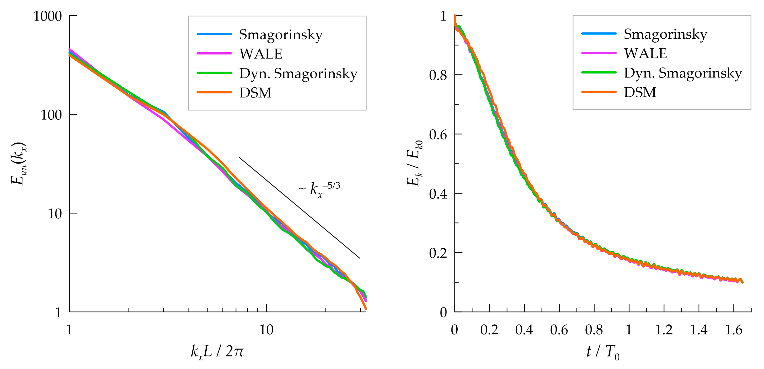
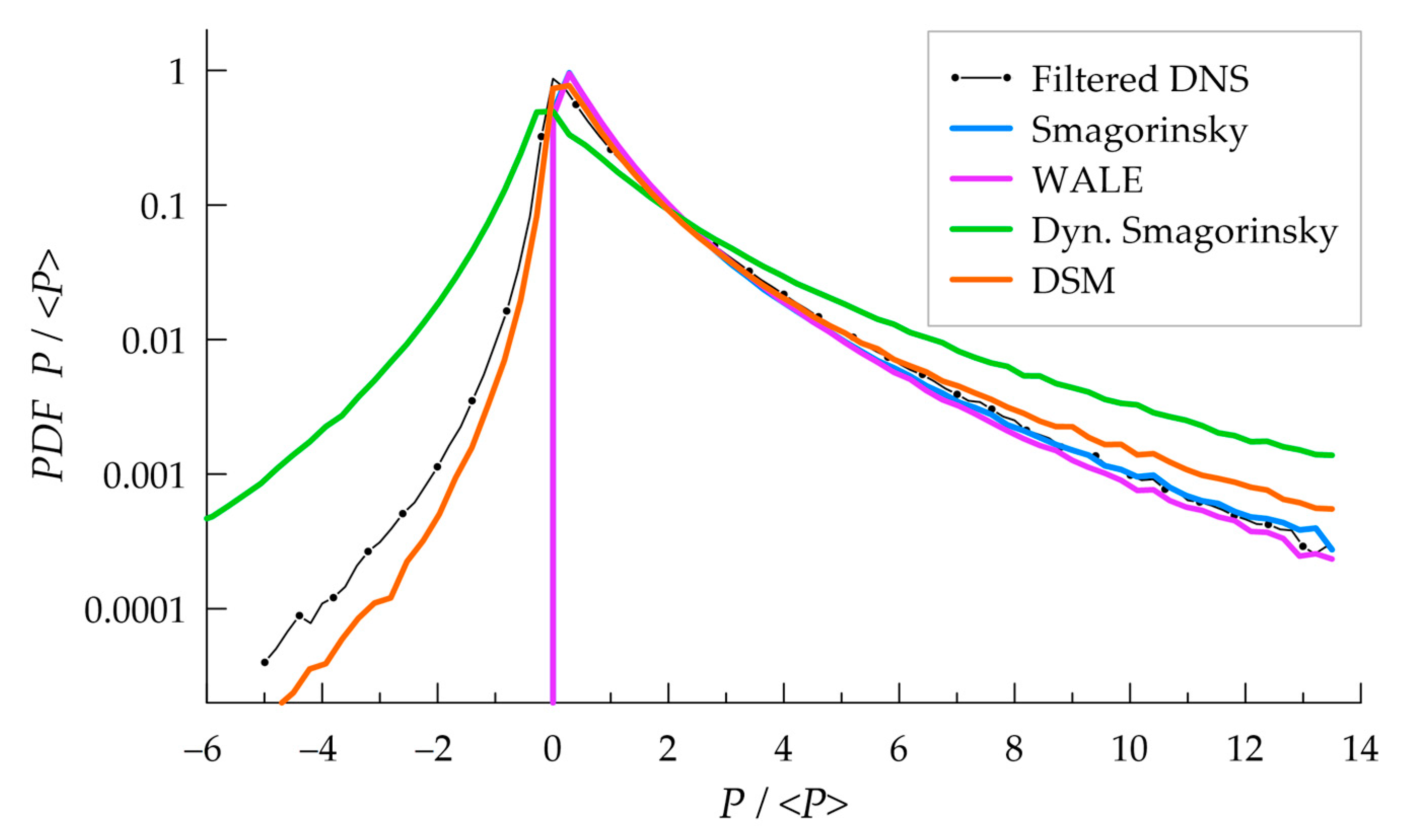
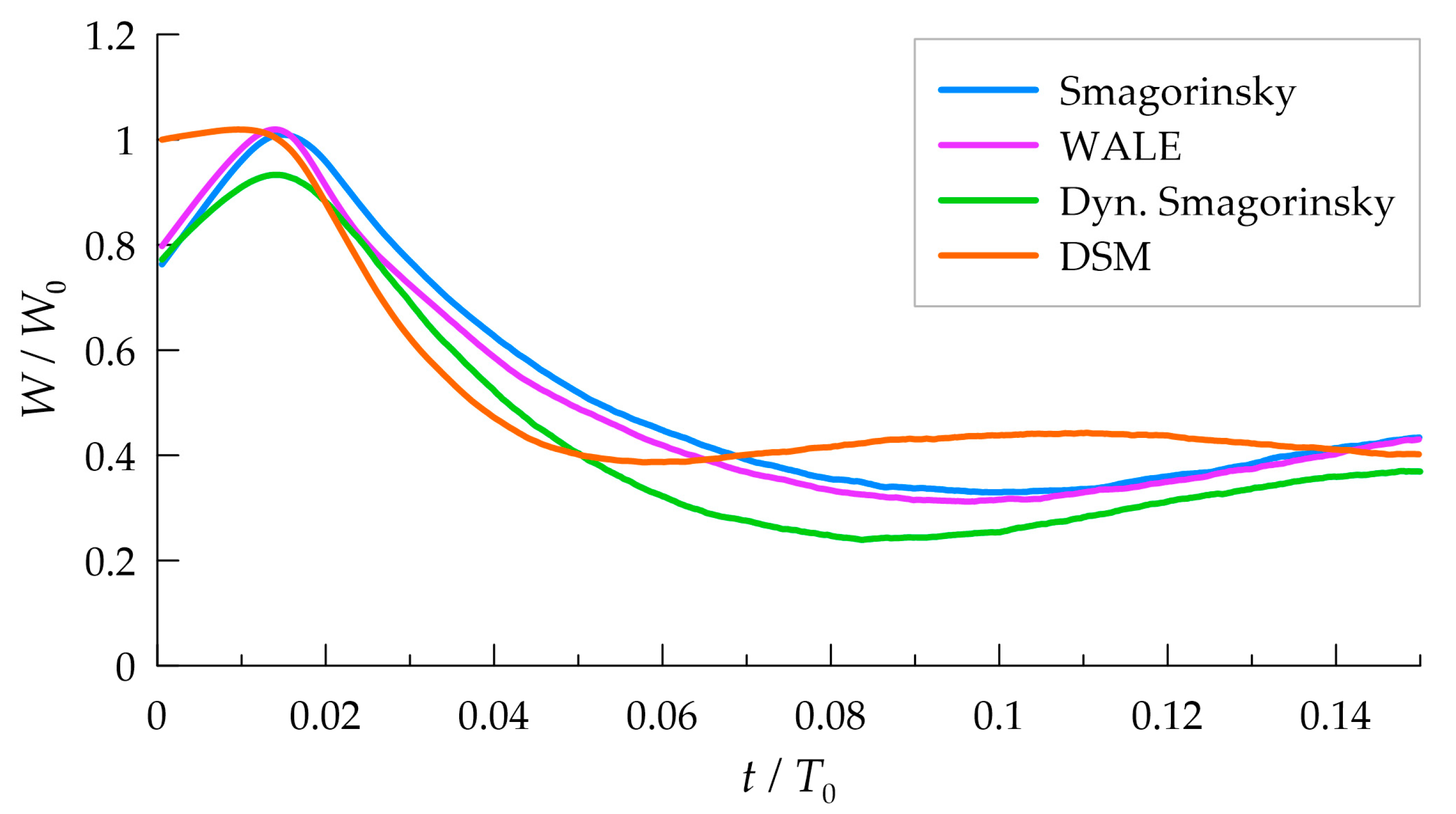
3.2. Subgrid Model Performance

To determine the constants in subgrid viscosity models, we conducted a series of simulations (only the first stages) in a computational domain of $64\times 64\times 64$ cells, varying the constants in the range $0.1\le C_s\le 0.2$, $-0.1\le C_{dyn}^{min}\le 0$, $0.05\le C_{dyn}^{max}\le 0.2$ and $0.3\le C_W\le 0.6$. We analyzed the longitudinal energy spectrum $E_{uu}\left(k_x\right)$ at the end of each simulation, as follows:

$$E_{uu}\left(k_x\right)={‹\left|{{\displaystyle \int }}_{-L/2}^{L/2}u\left(x, y, z\right)e^{-ıkx}dx\right|›}^2{}_{yz},$$

where $‹\dots {›}_{yz}$ denotes the averaging over all lines, $y, z=const$. The values corresponding to the Kolmogorov spectrum, $E_{uu}\left(k_x\right)\propto k_x^{-5/3}$, in the range of $7\le k_{x}L/2\pi \le 24$ were selected, which appeared to be equal to $C_s=0.13$, $C_{dyn}^{min}=-0.03$, $C_{dyn}^{max}=0.1$ and $C_W=0.4$. The same procedure was repeated for DSM, in which the ratio $\mathsf{\Delta }/H$ was varied ($H$ is the computational grid spacing first appeared in Equation (19)). The optimum choice was found to be $\mathsf{\Delta }=0.4 H$. In Figure 4, the optimal spectra are illustrated for all models along with the resolved kinetic energy decay. The oscillating character of energy is due to small dilatational motions present in the flow field. After a relaxation period of approximately $T_0/2$, the energy decays according to a power law of $E_k~t^{-1.1}$. All the models give similar statistics. However, this does not mean that the resolved fields are statistically equivalent. The energy decay rate and the energy spectrum correspond to the first two statistical moments of the velocity field. This is insufficient to fully describe the velocity field, e.g., its intermittency is left uncharacterized [3].

Interestingly, despite the discussed similarity in the resolved flow statistics, the subgrid turbulence behaves very differently with these models. At the end of the first stage, the Smagorinsky model predicts the volume-averaged subgrid kinetic energy to be $0.027E_{k1}$, the WALE model predicts it to be $0.030E_{k1}$, the dynamic Smagorinsky model gives $0.10E_{k1}$, while the DSM model gives $0.055E_{k1}$. The high value obtained with the dynamic Smagorinsky model was surprising to us. This may indicate that the choice of ${\nu }_{sgs}$ clipping in (20) is somewhat arbitrary and should be performed in some other way; another possible explanation is the use of $k$ clipping in (21), which tends to increase the volume-averaged $k$ value due to the presence of flow regions, where ${\nu }_{sgs}<0$. The DSM predicts the subgrid kinetic energy to be approximately two times higher than the Smagorinsky and WALE models. Most interestingly, DSM simulates backscatter regions where energy flux is locally directed from subgrid scales toward resolved ones which is consistent with experimental [2] and DNS [3] data. The same holds for the dynamic Smagorinsky model, although it overestimates the frequency of backscatter events. In Figure 5, the probability density functions of scale-to-scale energy flux $P=-\overline{u_i^{\prime }{u}_j^{\prime }} S_{ij}$ obtained with all models are plotted and compared with filtered DNS data. DSM is qualitatively correct in this distribution, which is encouraging while negative $P$ values are absent with Smagorinsky and WALE models. The dynamic Smagorinsky model predicts too wide distribution of the energy flux. Note that all models produce approximately the same volume-averaged energy flux which follows from the similarity of lines on the right of Figure 4.

The fact that the energy fluxes are close to each other while subgrid energies differ by a factor of 2 (not taking into account the dynamic Smagorinsky model) may be interpreted from the perspective of [3]. In [3], the authors analyzed the same DNS dataset as in the current paper and concluded that the turbulent cascade is relatively “ineffective” in transporting the energy across the scales. The principal axes of $\overline{u_i^{\prime }{u}_j^{\prime }}$ and $S_{ij}$ are statistically misaligned, which leads to a cascade efficiency of only 25% in the inertial range. In other words, a major part of the subgrid stresses drives spatial transport instead of participating in the spectral energy transfer. DSM can capture this effect due to the lack of algebraic connection between $\overline{u_i^{\prime }{u}_j^{\prime }}$ and $S_{ij}$. On the contrary, subgrid viscosity models align these tensors perfectly, which leads to errors in either energy transfer rate or in the subgrid stress levels.

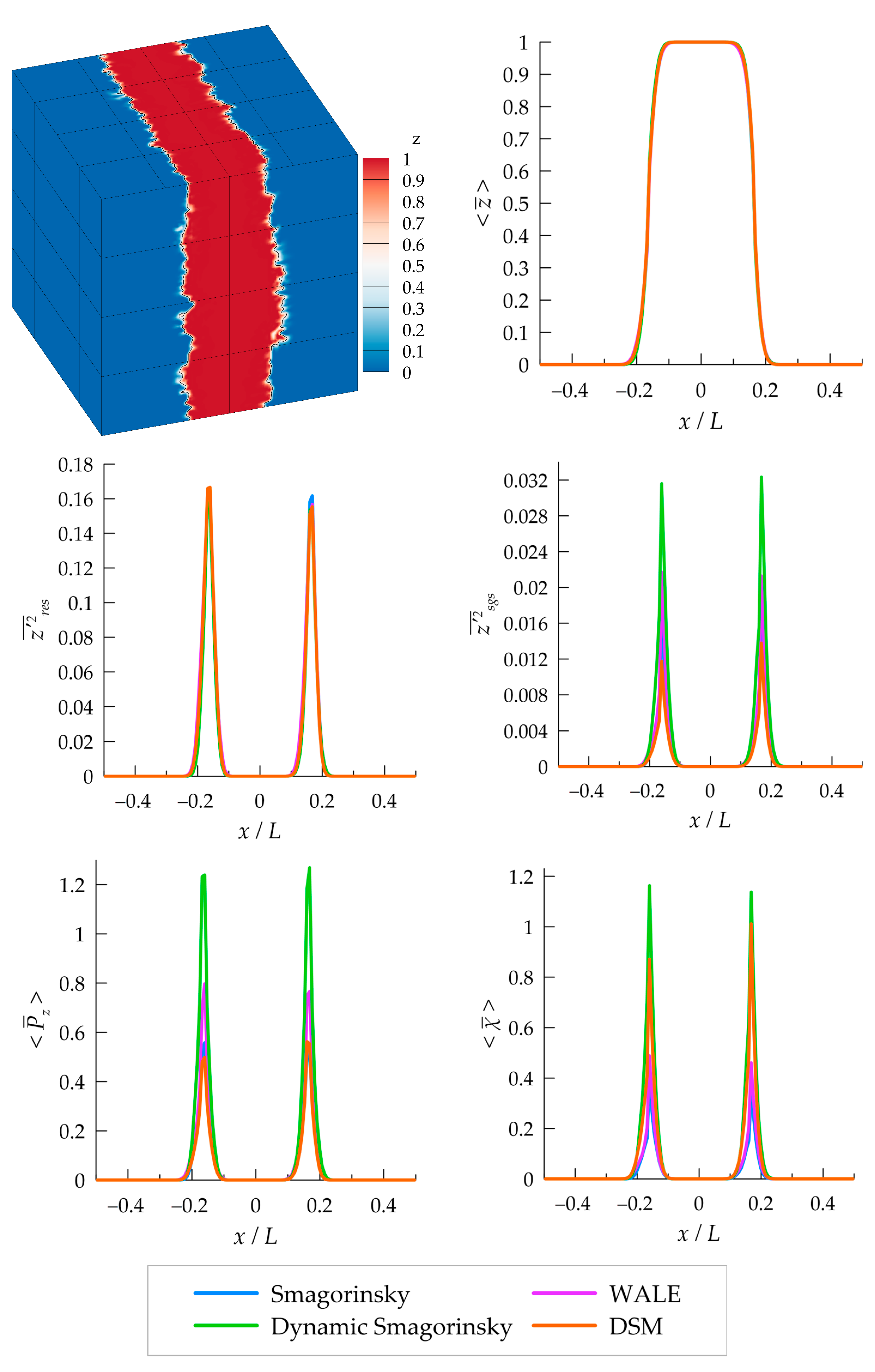
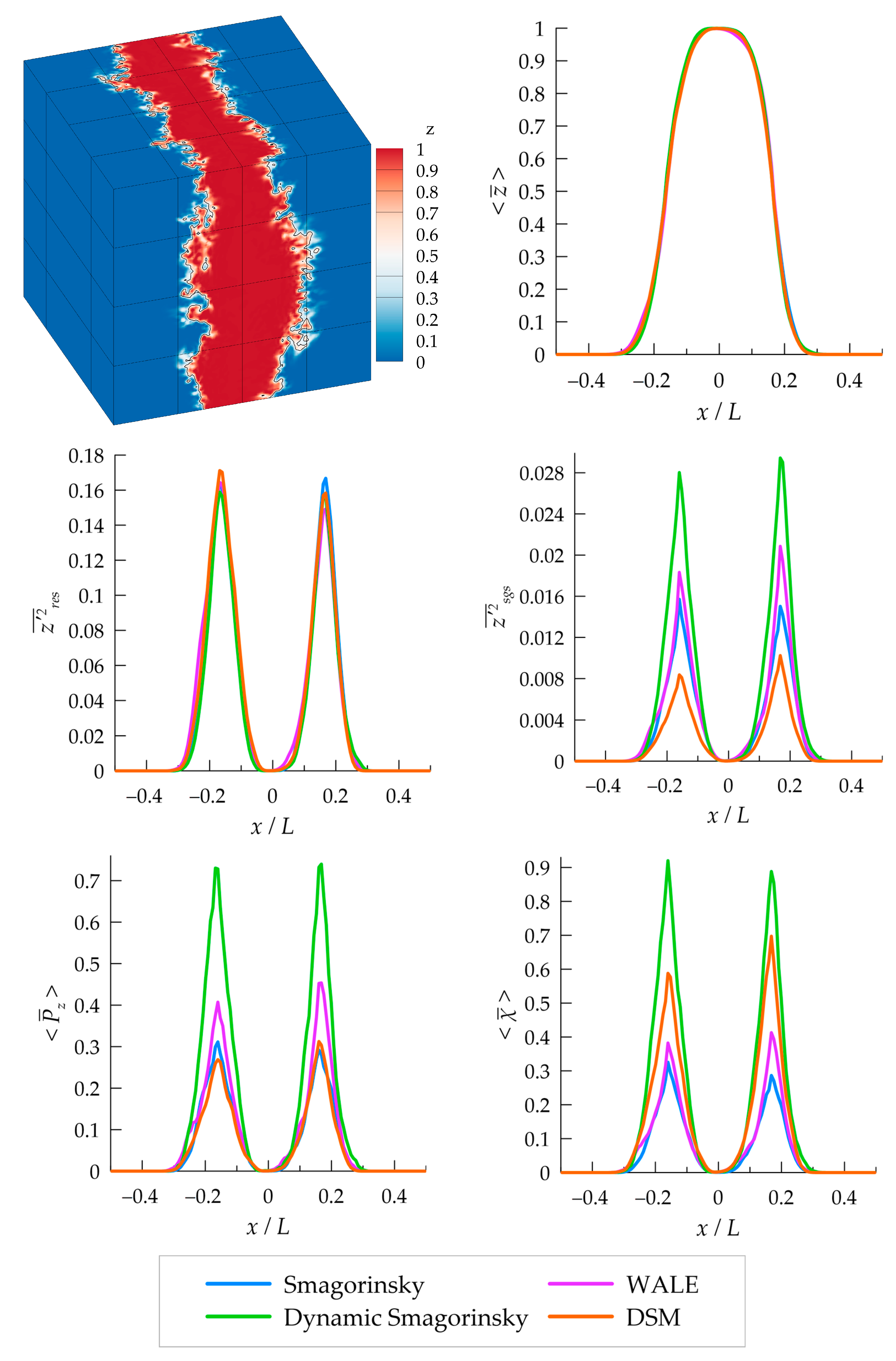
3.3. Mixture Fraction Statistics

In Figure 6, the fuel-consumption rate, $W=-d{M}_F/dt$, is shown where $M_F$ is the total fuel mass obtained by integrating the $\rho Y_F$ field over the volume of the computational domain. Consumption rate is normalized by $W_0$, an initial value of W in DSM simulation. It is seen that the profiles for all subgrid viscosity models are qualitatively similar while the DSM simulation departs from them near the start of the process and after $t/T_0=0.05$. The maximum ratio of fuel-consumption rates obtained with different models is as high as 1.8 at $t/T_0\approx 0.09$. This indicates the importance of accurate description of subgrid processes in the problem considered.

We selected four time instances, $t=\left\{0.02T_0, 0.05T_0, 0.1T_0, 0.15T_0\right\}$, for comparative analysis. Below (Figure 7, Figure 8, Figure 9 and Figure 10), we consider the instantaneous $\overline{z}$ field (black isoline corresponds to $\overline{z}=0.5$), ${‹\overline{z}›}_{YZ}\left(x\right)$, profile which is obtained by averaging $\overline{z}$ over YZ-planes, resolved mixture fractionmixture fraction variance ${\overline{z^{\prime 2}}}_{res}\left(x\right)=‹{\overline{z}}^2›{}_{YZ}-{‹\overline{z}›}_{YZ}^2$, subgrid-scale mixture fraction variance ${\overline{z^{\prime 2}}}_{sgs}\left(x\right)={‹\overline{z^{\prime 2}}›}_{YZ}$ and its production rate $‹{\overline{P}}_z›{}_{YZ}\left(x\right)$, and scalar dissipation ${‹\overline{\chi }›}_{YZ}\left(x\right)$. The last two statistics are calculated according to (26), (27).

Again, a comparison of the ${‹\overline{z}›}_{YZ}$ and ${\overline{z^{\prime 2}}}_{res}$ profiles shows that the resolved scalar statistics are similar with all the considered models. However, the subgrid-scale characteristics are significantly different. A typical level of mixture-fraction subgrid-scale variance is two times lower for the DSM than for the Smagorinsky model. A possible explanation of this difference is as follows. Consider a balance between production and dissipation of $\overline{z^{\prime 2}}$. In local equilibrium, ${\overline{P}}_z\approx \overline{\chi }$, so

$$2{\sigma }_{z1}\cdot {\nu }_{sgs}\cdot \frac{\partial \overline{z}}{\partial x_k}\frac{\partial \overline{z}}{\partial x_k}\approx C_{\chi }\frac{\sqrt{2.54{\nu }_{sgs}S}}{\mathsf{\Delta }}\overline{z^{\prime 2}} \Rightarrow \overline{z^{\prime 2}}\propto \sqrt{\frac{{\nu }_{sgs}}{S}}\mathsf{\Delta }\frac{\partial \overline{z}}{\partial x_k}\frac{\partial \overline{z}}{\partial x_k}\propto \frac{\mathsf{\Delta }}{H}.$$

In DSM, $\mathsf{\Delta }/H=0.4$, while in three other models, $\mathsf{\Delta }/H=1$. This leads to ${\left(\overline{z^{\prime 2}}\right)}_{DSM}/{\left(\overline{z^{\prime 2}}\right)}_{other}\approx 0.4$, which is even lower than the observed ratio of 0.5. To improve the estimate, one has to take into account the diffusion terms in $\overline{z^{\prime 2}}$ equation and the possible differences in the statistics of the $\partial \overline{z}/\partial x_k$ field, as predicted by different models.

These differences in the subgrid-scale characteristics may indicate that more advanced turbulent combustion models may behave very differently when employed with different classes of subgrid stress models. The DSM looks promising here because its subgrid stress field is not algebraically connected to the resolved strain field, which is more realistic compared with the subgrid viscosity models. This may be important in large eddy simulations of turbulent combustion with finite-reaction-rate chemistry.

4. Discussion and Conclusions

A new differential subgrid stress model (DSM) for large eddy simulations of turbulent flows was developed, a priori term-by-term calibrated and validated. For this purpose, an open DNS database [24,25] was used. The least squares method was found to be inappropriate due to its tendency to underestimate the modeled field norm. To avoid this problem, a new calibration method was proposed which maximizes the correlation coefficient of a modeled field while maintaining its correct norm. Even with this method, it was found that the calibrated model may appear to be unstable, so an appropriate choice of closure functional form is important in addition to determining the coefficient values. In the present study, only the inclusion of terms which were nonlinear in strain and rotation rates allowed us to stabilize the pressure–strain model. To our knowledge, all well-known pressure–strain models such as SSG [37] are linear in their mean (resolved) velocity gradients, which follows from the exact form of $\overline{p^{\prime }{S}_{ij}^{\prime }}$ in homogeneous turbulence. Thus, the new model can be considered as an extension of classical models to the inhomogeneous turbulence conditions found in the inertial range. Another result which we considered to be unexpected was the importance of the resolved velocity gradients in the triple-velocity correlation model (8). Although it is not a common practice to include such terms, this allowed us to increase the correlation coefficient from 0.3 to 0.85. The idea was inspired by [22], in which the importance of the velocity gradients in $\overline{u_i^{\prime }{u}_j^{\prime }{u}_k^{\prime }}$ closure was highlighted. The observations made in the current paper may be important for the development of future advanced subgrid stress models.

The model assessment was carried out in an LES of non-premixed turbulent combustion. The impact of the new subgrid stress model on the scalar fields was shown by a comparison of the DSM with the Smagorinsky, dynamic Smagorinsky and WALE models. There appeared to be no significant differences in the resolved velocity and mixture fraction fields, which may indicate that the backward influence of the subgrid scales on the resolved ones was relatively small in the considered problem. However, the new model was able to simulate backscatter in contrast to the Smagorinsky and WALE models, an effect observed in DNS. In the DSM, the backscatter relates to the misalignment between the principal axes of $\overline{u_i^{\prime }{u}_j^{\prime }}$ and $S_{ij}$. This misalignment also leads to the relative inefficiency of the turbulent energy cascade [3], which manifests itself as an increased subgrid stress level of DSM compared with the Smagorinsky and WALE models, while the energy transfer rate is approximately the same. The ability to capture such flow features may play a major role in more complex flows where backscatter is a flow-determining effect. Note that the backscatter is also captured by the dynamic Smagorinsky model, but in this case, it is caused by the presence of negative ${\nu }_{sgs}$ values. It was shown that the probability density function of energy flux obtained with the dynamic Smagorinsky model is too wide compared with the filtered DNS data.

Concerning the mixture fraction statistics, while their resolved parts behave similarly independent of a subgrid model, their subgrid parts significantly depend on the stress field. In the conducted simulations, the subgrid scalar variance was found to be two times lower with the DSM than with the Smagorinsky and WALE models. This was due to a smaller production term and a significantly larger scalar dissipation term. We believe that these differences may be important when advanced turbulence–combustion interaction models are employed.

References

1. Sagaut, P. Large Eddy Simulations of Incompressible Flows, 3rd ed.; Springer: Berlin, Germany, 2008; 558p. [Google Scholar]
2. Higgins, C.W.; Parlange, M.B.; Meneveau, C. Alignment trends of velocity gradients and subgrid-scale fluxes in the turbulent atmospheric boundary layer. Bound.-Layer Meteorol. 2003, 109, 59–83. [Google Scholar] [CrossRef]
3. Ballouz, J.G.; Ouellette, N.T. Tensor geometry in the turbulent cascade. J. Fluid Mech. 2018, 835, 1048–1064. [Google Scholar] [CrossRef]
4. Germano, M.; Piomelli, U.; Moin, P.; Cabot, W.H. A dynamic subgrid-scale eddy viscosity model. Phys. Fluids 1991, 3, 1760–1765. [Google Scholar] [CrossRef]
5. Zang, Y.; Street, R.L.; Koseff, J.R. A dynamic mixed subgrid-scale model and its application to turbulent recirculating flows. Phys. Fluids A 1993, 5, 3186–3196. [Google Scholar] [CrossRef]
6. Zhao, H.; Voke, P.R. A dynamic subgrid-scale model for low-Reynolds-number channel flow. Int. J. Numer. Methods Fluids 1996, 23, 19–27. [Google Scholar] [CrossRef]
7. Montecchia, M.; Brethouwer, G.; Johansson, A.V.; Wallin, S. Taking large-eddy simulation of wall-bounded flows to higher Reynolds numbers by use of anisotropy-resolving subgrid models. Phys. Rev. Fluids 2017, 2, 034601. [Google Scholar] [CrossRef]
8. Troshin, A.; Bakhne, S.; Sabelnikov, V. Numerical and physical aspects of large-eddy simulation of turbulent mixing in a helium-air supersonic co-flowing jet. In Progress in Turbulence IX. iTi 2021; Örlü, R., Talamelli, A., Peinke, J., Oberlack, M., Eds.; Springer: Cham, Switzerland, 2021; pp. 297–302. [Google Scholar] [CrossRef]
9. Deardorff, J.W. The use of subgrid transport equations in a three-dimensional model of atmospheric turbulence. J. Fluids Eng. 1973, 95, 429–438. [Google Scholar] [CrossRef]
10. Fureby, C.; Tabor, G.; Weller, H.G.; Gosman, A.D. Differential subgrid stress models in large eddy simulations. Phys. Fluids 1997, 9, 3578–3580. [Google Scholar] [CrossRef]
11. Zhuchkov, R.N.; Utkina, A.A. Combining the SSG/LRR-ω differential Reynolds stress model with the detached eddy and laminar-turbulent transition models. Fluid Dyn. 2016, 51, 733–744. [Google Scholar] [CrossRef]
12. Liu, Y.; Zhou, Z.; Zhu, L.; Wang, S. Numerical investigation of flows around an axisymmetric body of revolution by using Reynolds-stress model based hybrid Reynolds-averaged Navier–Stokes/large eddy simulation. Phys. Fluids 2021, 33, 085115. [Google Scholar] [CrossRef]
13. Wang, G.; Wang, S.; Li, H.; Fu, X.; Liu, W. Comparative assessment of SAS, IDDES and hybrid filtering RANS/LES models based on second-moment closure. Adv. Mech. Eng. 2021, 13, 1–14. [Google Scholar] [CrossRef]
14. Smagorinsky, J. General circulation experiments with the primitive equations: I. The basic experiment. Mon. Weather Rev. 1963, 91, 99–164. [Google Scholar] [CrossRef]
15. Nicoud, F.; Ducros, F. Subgrid-scale stress modelling based on the square of the velocity gradient tensor. Flow Turbul. Combust. 1999, 62, 183–200. [Google Scholar] [CrossRef]
16. Cook, A.W.; Riley, J.J.; Kosály, G. A laminar flamelet approach to subgrid-scale chemistry in turbulent flows. Combust. Flame 1997, 109, 332–341. [Google Scholar] [CrossRef]
17. Williams, F.A. Combustion Theory, 2nd ed.; CRC Press: Boca Raton, FL, USA, 2018; 708p. [Google Scholar]
18. Peters, N. Laminar diffusion flamelet models in non-premixed turbulent combustion. Prog. Energy Combust. Sci. 1984, 10, 319–339. [Google Scholar] [CrossRef]
19. Rota, G.-C. On the combinatorics of cumulants. J. Comb. Theory Ser. A 2000, 91, 283–304. [Google Scholar] [CrossRef]
20. Germano, M. A proposal for a redefinition of the turbulent stresses in the filtered Navier–Stokes equations. Phys. Fluids 1986, 29, 2323–2324. [Google Scholar] [CrossRef]
21. Hanjalić, K.; Launder, B. Modelling Turbulence in Engineering and the Environment; Cambridge University Press: Cambridge, UK, 2011; 402p. [Google Scholar]
22. Younis, B.A.; Gatski, T.B.; Speziale, C.G. Towards a rational model for the triple velocity correlations of turbulence. Proc. R. Soc. Lond. A 2002, 456, 909–920. [Google Scholar] [CrossRef]
23. Lumley, J.L. Computational modeling of turbulent flows. Adv. Appl. Mech. 1979, 18, 123–176. [Google Scholar] [CrossRef]
24. Li, Y.; Perlman, E.; Wan, M.; Yang, Y.; Meneveau, C.; Burns, R.; Chen, S.; Szalay, A.; Eyink, G. A public turbulence database cluster and applications to study Lagrangian evolution of velocity increments in turbulence. J. Turbul. 2008, 9, N31. [Google Scholar] [CrossRef]
25. Available online: http://turbulence.pha.jhu.edu/ (accessed on 4 July 2022).
26. Menter, F.R.; Garbaruk, A.V.; Egorov, Y. Explicit algebraic Reynolds stress models for anisotropic wall-bounded flows. In Proceedings of the 3rd European Conference for Aero-Space Sciences, Versailles, France, 6–9 July 2009. [Google Scholar]
27. Lily, D.K. The representation of small-scale turbulence in numerical simulation experiments. In Proceedings of the IBM Scientific Computing Symposium on Environmental Sciences, Yorktown Heights, NY, USA, 14–16 November 1966; IBM Form No. 320-1951. pp. 195–210. [Google Scholar]
28. Canuto, V.M.; Cheng, Y. Determination of the Smagorinsky–Lilly constant CS. Phys. Fluids 1997, 9, 1368–1378. [Google Scholar] [CrossRef]
29. Jameson, A. Formulation of kinetic energy preserving conservative schemes for gas dynamics and direct numerical simulation of one-dimensional viscous compressible flow in a shock tube using entropy and kinetic energy preserving schemes. J. Sci. Comput. 2008, 34, 188–208. [Google Scholar] [CrossRef]
30. Lambert, J.D. Computational Methods in Ordinary Differential Equations (Introductory Mathematics for Scientists and Engineers); John Wiley & Sons: Hoboken, NJ, USA, 1973; 278p. [Google Scholar]
31. Shur, M.L.; Spalart, P.R.; Strelets, M.K.; Travin, A.K. Synthetic turbulence generators for RANS-LES interfaces in zonal simulations of aerodynamic and aeroacoustic problems. Flow Turbul. Combust. 2014, 93, 63–92. [Google Scholar] [CrossRef]
32. Peters, N. Turbulent Combustion; Cambridge University Press: Cambridge, UK, 2000; 324p. [Google Scholar]
33. NIST/SEMATECH e-Handbook of Statistical Methods. Available online: https://itl.nist.gov/div898/handbook/eda/section3/eda366h.htm (accessed on 4 July 2022).
34. Poinsot, T.; Veynante, D. Theoretical and Numerical Combustion, 2nd ed.; RT Edwards: Philadelphia, PA, USA, 2005; 538p. [Google Scholar]
35. Lien, F.S.; Liu, H.; Chui, E.; McCartney, C.J. Development of an analytical β-function pdf integration algorithm for simulation of non-premixed turbulent combustion. Flow Turbul. Combust. 2009, 83, 205–226. [Google Scholar] [CrossRef]
36. Available online: https://www.boost.org/ (accessed on 4 July 2022).
37. Speziale, C.G.; Sarkar, S.; Gatski, T.B. Modelling the pressure–strain correlation of turbulence: An invariant dynamical systems approach. J. Fluid Mech. 1991, 227, 245–272. [Google Scholar] [CrossRef]
Figure 1. Radial kinetic energy spectrum in DNS and different filter cut-off scales.
Applsci 12 08491 g001
Figure 2. Iteration process scheme: correlation coefficient contour and b ˜ 1 = b 1 isoline are shown.
Applsci 12 08491 g002
Figure 3. CE probability density function for Δ = 256 h The region on the left corresponding to 1% of total probability is shown in red.
Applsci 12 08491 g003
Figure 4. Longitudinal spectra at the end of the first stage (left) and resolved kinetic energy evolution during the first stage (right).
Applsci 12 08491 g004
Figure 5. Normalized probability density function of scale-to-scale energy flux.
Applsci 12 08491 g005
Figure 6. Fuel-consumption rate.
Applsci 12 08491 g006
Figure 7. Time instance t = 0.02T0. Instantaneous z ¯ field obtained with the DSM (upper left), z ¯ Y Z ( x ) (upper right), z 2 ¯ r e s (middle left), z 2 ¯ s g s (middle right), P ¯ z Y Z ( x ) (lower left), χ ¯ Y Z ( x ) (lower right).
Applsci 12 08491 g007
Figure 8. Time instance t = 0.05T0. Designations as in Figure 7.
Applsci 12 08491 g008
Figure 9. Time instance t = 0.10T0. Designations as in Figure 7.
Applsci 12 08491 g009
Figure 10. Time instance t = 0.15T0. Designations as in Figure 7.
Applsci 12 08491 g010