Article

Integrated Adaptive Steering Stability Control for Ground Vehicle with Actuator Saturations

1
School of Mechanical and Electrical Engineering, Guangzhou University, Guangzhou 510006, China
2
School of New Energy, Nanjing University of Science and Technology, Jiangyin 214331, China
*
Author to whom correspondence should be addressed.
These authors contributed equally to this work.
Appl. Sci. 2022, 12(17), 8502; https://doi.org/10.3390/app12178502
Submission received: 14 July 2022 / Revised: 17 August 2022 / Accepted: 24 August 2022 / Published: 25 August 2022

Abstract

:
During a steering manoeuvre in a ground vehicle, both yaw motion and roll motion can occur simultaneously, and their dynamics can be coupled, as the roll motion is generalized directly from the tires’ lateral force under steering. Hence, it is of significance to analyze them as an integrated plant in the vehicle steering stability control problem. Furthermore, the actuator saturation of yaw control cannot be neglected, as vehicles often steer at a high velocity or on low-friction roads. In this paper, an integrated steering dynamics model is established considering the coupling between the roll motion and lateral motion, then a novel nonlinear adaptive controller is proposed to stabilize the steering motion considering the actuator saturation of yaw motion control. Simulation results indicate that the designed integrated controller is effective in improving the performance of both the yaw rate tracking error and ride comfort taking into account vehicle parameter uncertainties and actuator saturation; the steering stability of ground vehicles can consequently be guaranteed.

1. Introduction

In a steering manoeuvre for a ground vehicle, yaw motion can be generated directly [1,2]. When the vehicle is moving a a high velocity during a steering manoeuvre, unstable sideslip or even drift may occur, which is a dangerous working condition as the vehicle cannot be controlled easily by the driver [3,4]. Consequently, steering stability control is imperative. Conventionally, two signals are taken as controlled states; one is yaw rate, which represents manoeuvrability, while the other is the sideslip angle, denoting lateral stability [5] A novel triple-step nonlinear method was designed for steering stability control of in-wheel motor electric vehicles in [6], realizing the decoupling of the yaw rate and sideslip angle nonlinear dynamics. There have been many steering stability control methods proposed, including the aforementioned paper and others [7,8,9]; while the control results to date have been brilliant, no influence on vehicle roll motion from steering motion is considered in the extant literature. As is well known from experience, vehicle steering can result in body roll motion, which is related to passenger ride comfort.
As os known, an effective approach to improving passenger ride comfort is an active suspension system (ASS), the principle of which is to isolate the vibration of the unsprung mass to the vehicle body [10,11]. The classical ASS controller is designed based on a quarter-vehicle model [12]. In [13], a multi-objective control was derived for an uncertain nonlinear ASS, taking into account both the dynamic tire load and suspension space. However, the roll motion cannot be handled by a quarter-vehicle model despite the favorable isolation effect of the unsprung mass vibration. Often, vehicle roll stability control is involved in vehicle attitude control, for which a full-car model is most often employed. An adaptive robust ASS controller was develop in [14] using a full-car model, with the roll stability is taken as one of the control targets. The aforementioned roll stability control presents excellent roll stability performance; nevertheless, the roll dynamics effect from vehicle steering is not involved. Therefore, a nominal roll stability controller that does not consider the effect from steering may not work as desired.
Several researchers have focused on integrated steering stability control. In [15,16], the authors employed a linear quadratic regulator and a sliding mode control method to simultaneously control roll and yaw motion, respectively. A nonlinear control law was designed in [17] to follow the desired trajectories of both yaw and roll behaviours. In [18,19], the authors used model predictive control to simultaneously regulate yaw motion and stabilize roll motion. Similarly, feedback linearization methods have been utilized to solve the coupled yaw–roll motion problem in [20,21]. Although these techniques can handle integrated steering control remarkably well, actuator saturation has not yet been considered. Generally, the yaw stability control moment is realized by active steering or differential braking. When a ground vehicle steers on a low friction road or with a large yaw rate, the tire–road utilized adhesion force cannot supply enough control energy for its physical limitations, which means that saturation of the actuator effort (the active steering angle or braking force) occurs. Hence, it is important to consider the actuator saturation of yaw control in the development of controller design. Two approaches are available to handle actuator saturation: the first is the one-step approach, in which actuator saturation is taken as a constraint in the controller design process [22,23]; the other is two-step approach, in which the nominal controller is designed first, than an anti-windup compensator is designed to handle the actuator saturation [24,25]. Here, we mentions a few approaches: an anti-windup compensator in the form of a filter was designed for an attitude controller in spacecraft under input saturation and measurement uncertainty in [26,27], an auxiliary anti-windup compensator system was introduced to analyze the effect of the input constraint in a saturated robust adaptive backstepping controller design; finally, in this paper, a two-step approach controller is designed to handle actuator saturation.
Based on the aforementioned analysis, a steering stability control system integrating yaw, roll, and lateral and heave movement behaviours with actuator saturation and vehicle parameter perturbations has not previously been studied simultaneously and thoroughly. Thus, an integrated steering stability controller is developed in this paper, taking into consideration parameter perturbations and saturation of the yaw control effort. The main contributions of this paper are summarized as follows: (i) based on the integrated dynamics model, an integrated adaptive steering stability controller is proposed to stabilize the yaw, roll, heave, and lateral motion simultaneously with parameter perturbations; (ii) the actuator saturation of the yaw moment is considered in the context of integrated controller development; hence, the designed controller can guarantee tracing performance of the yaw rate with less degradation.
The rest of this paper is organized as follows: we establish the integrated dynamics model and the analysis of the coupling principle in Section 2; then, we describe the design of an integrated steering stability controller considering the actuator saturation of yaw control in Section 3. In Section 4, a numerical simulation is carried out to verify the effectiveness of the designed controller, followed by our conclusions in Section 5.

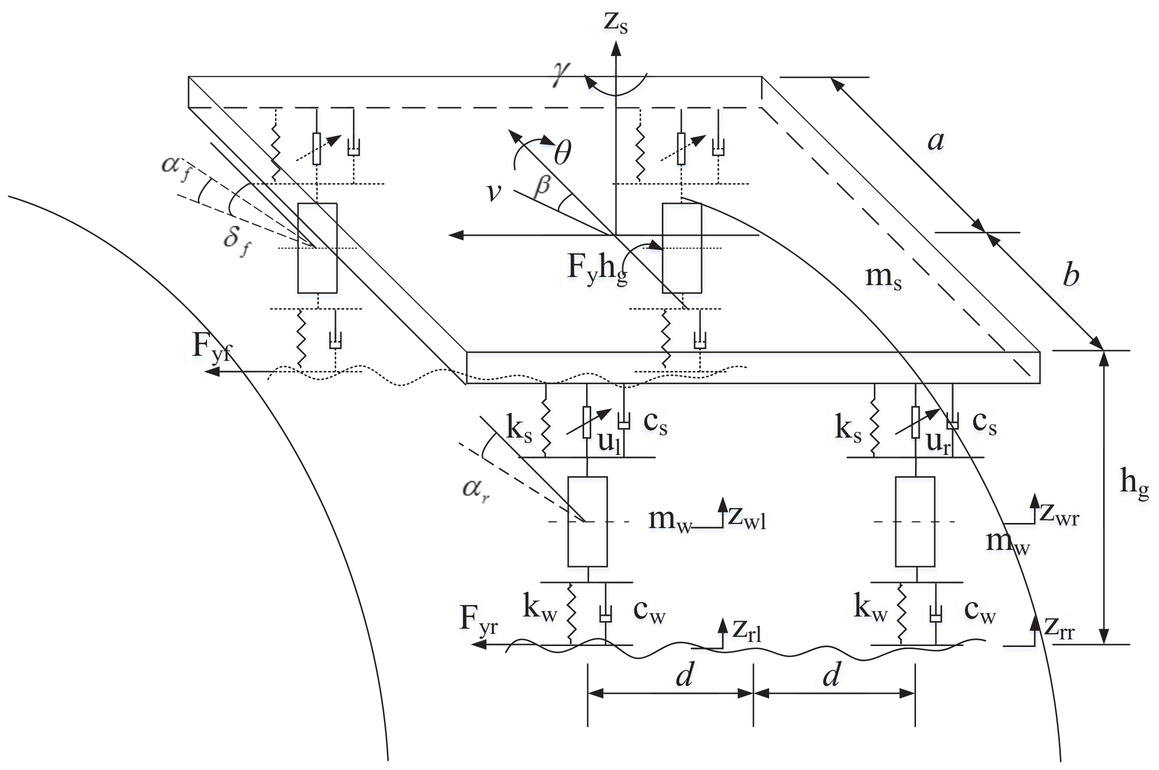
2. Problem Formulation

During a turning manoeuvre by a vehicle, both yaw movement and roll movement are brought about; a 6-DOF turning dynamics model considering heave and roll movement of the sprung mass, left and right hop movement of the unsprung mass, and lateral and yaw movement of the whole vehicle is established in Figure 1, where z s and θ are the vertical displacement and roll angle, respectively, of the sprung mass, z w l and z w r are the respective hop of the left and right unsprung mass, z r l and z r r are the respective vertical inputs of the left and right road, β and γ are the respective slip angle and yaw rate of the whole vehicle, m s is the sprung mass, v is the vehicle velocity, F y is the total lateral force of the four tires, h g is the height of CG, k s and c s are the stiffness and damping coefficient of the unilateral (left or right, hereinafter) suspension springs and dampers, respectively, k w and c w are the respective stiffness and damping coefficient of the unilateral tire springs and dampers, m w is the unilateral mass of the unsprung mass, F y l and F y r are the respective lateral force of left and right tires, d is the half-tread, α f and α r are the respective slip angles of the front and rear wheels, δ f is the steering angle of front wheel, a and b are the distance from the CG of the sprung mass to the front axle and rear axle, respectively, u z and u θ are respectively the equivalent vehicle body vertical force and roll moment, which are essentially determined by u l and u r , and u l and u r are the respective input forces of the left and right active suspensions. Conventionally, the control input forces u l and u r can be generated by linear electric motors.
The corresponding dynamics can be formulated as follows:
m s z ¨ s + F s d l + F s d r + F s s l + F s s r = u z
I x θ ¨ + d ( F s d l + F s s l ) d ( F s d r + F s s r ) = u θ + F y h g
m w z ¨ w l F s d l F s s l + F w d l + F w s l = u l
m w z ¨ w r F s d r F s s r + F w d r + F w s r = u r
β ˙ = 2 ( c f + c r ) m v β + 2 ( b c r a c f ) m v 2 1 γ + 2 c f m v δ f
γ ˙ = 2 ( b c r a c f ) I z β 2 ( a 2 c f + b 2 c r ) I z v γ + 2 a c f I z δ f + 1 I z M
where
F w d l = c w ( z ˙ w l z ˙ r l ) F w d r = c w ( z ˙ w r z ˙ r r ) F w s l = k w ( z w l z r l ) F w s r = k w ( z w r z r r ) , F s d l = c s Δ y ˙ l F s d r = c s Δ y ˙ r F s s l = k s Δ y l F s s r = k s Δ y r , Δ y l = z s + d sin θ z w l Δ y r = z s d sin θ z w r Δ y ˙ l = z ˙ s + d θ ˙ cos θ z ˙ w l Δ y ˙ r = z ˙ s d θ ˙ cos θ z ˙ w r ,
F y = F y f cos δ f + F y r = 2 c f α f cos δ f + 2 c r α r ,
K = m 2 L 2 ( b c f a c r ) , L = a + b , m = m s + 2 m w ,
u l + u r = u z u l d u r d = u θ , α f = δ f a γ v β α r = b γ v β ,
where F w d l and F w d r are the respective damper forces of the left tire and right tire, F w s l and F w s r are the respective spring forces of the left tire and right tire, F s d l and F s d r are the respective damper forces of the left tire and right suspension, F s s l and F s s r are the respective spring forces of the left tire and right suspension, Δ y l and Δ y r are the dynamic deflection of the left and right suspension, respectively, c f and c r are the respective cornering stiffnesses of the single front and rear tires, L is the wheelbase, M is the yaw moment control input, which can be generated either by active wheel steering or braking force, and I z and I x are the respective inertial yaw and roll moments. For more detailed information about the physical meanings of these notations, readers can refer to [16,17,28] and the references therein.
The control problem can be depicted as follows: lim t z s 0 or bounded, lim t θ 0 or bounded, and lim t ( γ γ r ) 0 or bounded, under the condition that z w l , z w r and β are bounded; γ r is the reference yaw rate, which can be formulated as γ r = v v L L 1 + K v 2 δ f .

3. Integrated Controller Design

Let x 1 = z s , x 2 = z ˙ s , x 3 = θ , x 4 = θ ˙ , x 5 = z w l , x 6 = z ˙ w l , x 7 = z w r , x 8 = z ˙ w r , x 9 = β , and x 10 = γ ; then, the vehicle dynamics can be reformulated as
x ˙ 1 = x 2 , x ˙ 2 = 1 m s ( F s d l F s d r F s s l F s s r + u z ) x ˙ 3 = x 4 , x ˙ 4 = 1 I x ( d ( F s d l + F s s l ) + d ( F s d r + F s s r ) + F y h g + u θ ) x ˙ 5 = x 6 , x ˙ 6 = 1 m w l ( F s d l + F s s l F w d l F w s l u l ) x ˙ 7 = x 8 , x ˙ 8 = 1 m w r ( F s d r + F s s r F w d r F w s r u r ) x ˙ 9 = 2 ( c f + c r ) m v x 9 + 2 ( b c r a c f ) m v 2 1 x 10 + 2 c f m v δ f x ˙ 10 = 2 ( b c r a c f ) I z x 9 2 ( a 2 c f + b 2 c r ) I z v x 10 + 2 a c f I z δ f + 1 I z M
Accordingly, the integrated controller can be synthesised via the following three steps. Step 1: let e 1 = x 1 x 1 r , and e 2 = x 2 x 2 r , where x 1 r is the reference value of x 1 and x 2 r is the virtual control input; then,
e ˙ 1 = x ˙ 1 x ˙ 1 r = e 2 + x 2 r x ˙ 1 r .
Choose V 1 = 1 2 e 1 2 as a Lyapunov candidate; its derivation along e ˙ 1 yields
V ˙ 1 = e 1 ( e 2 + x 2 r x ˙ 1 r )
Take x 2 r = x ˙ 1 r k 1 e 1 , where k 1 > 0 is the design parameter; then, we have
V ˙ 1 = e 1 e 2 k 1 e 1 2 .
Choose V 2 = V 1 + m s 2 e 2 2 + 1 2 r 1 m ˜ s 2 as a Lyapunov candidate, where m ˜ s = m ^ s m s and m ^ s is the estimation value of m s ; then, taking its deviation yields
V ˙ 2 = e 1 e 2 k 1 e 1 2 + e 2 ( F s d l F s d r F s s l F s s r + u z m s x ˙ 2 r ) + 1 r 1 m ˜ s m ^ ˙ s .
Take
u z = F s d l + F s d r + F s s l + F s s r + m ^ s x ˙ 2 r k 2 e 2 e 1
and the adaptation law
m ^ ˙ s = r 1 e 2 x ˙ 2 r ,
where k 2 > 0 and r 1 > 0 are design parameters; then, we have
V ˙ 2 = k 1 e 1 2 k 2 e 2 2 0
which indicates that e 1 , e 2 and m ˜ s are bounded. Taking the derivative of V ˙ 2 leads to
V ¨ 2 = 2 k 1 e 1 ( e 2 + x 2 r ) 2 k 2 e 2 ( 1 m s ( F s d l F s d r F s s l F s s r + u z ) x ˙ 2 r ) ,
thus, V ˙ 2 is uniformly continuous, conditional on x 1 r and x ˙ 1 r L . Consequently, the error dynamics of e 1 and e 2 are asymptotically convergent to 0 with Lyapunov-like lemma.
Step 2: to facilitate the development of the control law, the following simplicities are used: θ I = 1 I x and f θ ( x θ , δ f ) = d ( F s d l + F s s l ) + d ( F s d r + F s s r ) + F y h g , where x θ = ( x 1 , x 2 , x 3 , x 4 , x 5 , x 6 , x 7 , x 8 ) T . Let e 3 = x 3 x 3 r , e 4 = x 4 x 4 r , θ ˜ I = θ ^ I θ I , where x 3 r is the reference value of x 3 , x 4 r is the virtual control input, and θ ^ I is the estimation of θ I . Following a similar procedure as in Step 2, we can choose V 4 = 1 2 e 3 2 + 1 2 e 4 2 + 1 2 r 2 θ ˜ I 2 as a Lyapunov function and take
x 4 r = x ˙ 3 r k 3 e 3
u θ = f θ ( x θ , δ f ) + 1 θ ^ I ( x ˙ 4 r k 4 e 4 e 3 )
with the projection-type adaptation law [29,30,31]:
θ ^ ˙ I = P r o j θ ^ I ( r 2 e 4 ( f θ ( x θ , δ f ) + u θ ) ) = 0 i f θ ^ I = θ I max a n d r 2 e 4 ( f θ ( x θ , δ f ) + u θ ) > 0 0 i f θ ^ I = θ I min a n d r 2 e 4 ( f θ ( x θ , δ f ) + u θ ) < 0 r 2 e 4 ( f θ ( x θ , δ f ) + u θ ) o t h e r w i s e
where k 3 > 0 , k 4 > 0 and r 2 > 0 are design parameters, and θ I max and θ I min are the known maximum and minimum values of θ I ; then, we have
V ˙ 4 = k 3 e 3 2 k 4 e 4 2 0 .
Thus, e 3 , e 4 , and θ ˜ I are bounded; taking the derivative of V ˙ 4 further yields V ¨ 4 = 2 k 3 e 3 ( e 4 + x 4 r ) 2 k 4 e 4 ( θ I ( f θ ( x θ , δ f ) + u θ ) x ˙ 4 r ) , which is bounded on the condition that x ˙ 3 r is bounded. Hence, V ˙ 4 is uniformly continuous, and consequently e 3 , e 4 0 , as t with Lyapunov-like lemma.
After u z and u θ are determined, the active suspension control input can be obtained as follows:
u l = d u z + u θ 2 d , u r = d u z u θ 2 d .
Step 3: for simplicity, let f γ ( x γ , δ f ) = 2 ( b c r a c f ) x 9 2 ( a 2 c f + b 2 c r ) v x 10 + 2 a c f δ f , where x γ = ( x 9 , x 10 ) T ; then, Equation (7) can be simplified as
x ˙ 10 = 1 I z ( f γ ( x γ , δ f ) + M )
where the saturated control input can be presented as
M = s a t ( u y ) = sgn ( u y ) · min { u y , u max } ,
where u y is the actuator demand input, s a t ( u y ) is the actuator actual output, and u m a x > 0 is the positive upper bound of the actuator.
We now take the state tracing error of x 10 as e 10 = x 10 x 10 r , where x 10 r is the reference value of x 10 . Let M Δ = M u y , and pass it through a filter ζ ˙ = k ζ ζ + M Δ , where k ζ is the tuning parameter. The filter acts as an anti-windup compensator, thus, the actuator saturation M Δ can be canceled out by feeding ζ back into the nominal control input, u y [26].
Choosing a Lyapunov candidate V 10 = I z 2 e 10 2 + 1 2 ζ 2 , we then have
V ˙ 10 = e 10 ( f γ ( x γ , δ f ) + M Δ + u y I z x ˙ 10 r ) k ζ ζ 2 + ζ M Δ
We design the control law of u y as
u y = f γ ( x γ , δ f ) + I z x ˙ 10 r k 10 e 10 k 11 ζ , k 10 > 0 .
Then, substituting (16) into (15) yields
V ˙ 10 = k 10 e 10 2 k ζ ζ 2 + e 10 M Δ k 11 ζ e 10 + ζ M Δ = k 10 3 e 10 2 + ( e 10 M Δ k 10 3 e 10 2 ) + ( k 10 3 e 10 2 k ζ 3 ζ 2 k 11 ζ e 10 ) k ζ 3 ζ 2 + ( ζ M Δ k ζ 3 ζ 2 ) = k 10 3 e 10 2 ( k 10 3 e 10 3 4 k 10 M Δ ) 2 + 3 4 k 10 M Δ 2 1 2 ( k 11 e 10 + k 11 ζ ) 2 ( k 11 2 + k 10 3 ) e 10 2 ( k 11 2 + k ζ 3 ) ζ 2 k ζ 3 ζ 2 ( k ζ 3 ζ 3 4 k ζ M Δ ) 2 + 3 4 k ζ M Δ 2 ( 2 k 10 3 k 11 2 ) e 10 2 ( 2 k ζ 3 k 11 2 ) ζ 2 + ( 3 4 k 10 + 3 4 k ζ ) M ¯ 2
where M ¯ is the upper bound of M Δ . If we take ρ = min { 4 k 10 3 k 11 3 I z , 4 k ζ 3 k 11 } , 2 k 10 3 > k 11 2 , and 2 k ζ 3 > k 11 2 , then
V ˙ 10 ρ V 10 + ε
where ε = ( 3 4 k 10 + 3 4 k ζ ) M ¯ 2 . Integrating both sides of (17) generates
V 10 ( t ) ε ρ + ( V 10 ( 0 ) ε ρ ) e ρ t
When t , we have V ( ) ε 0 ρ , meaning that the signals e 10 and ζ are ultimately bounded and the attraction domain of V 10 can be adjusted to be smaller, with a smaller σ and a larger k 10 .
The integrated controller design yields a fifth-order error dynamics system, while the original system is a tenth-order system. Hence, the zero dynamics contains five states. Setting e 1 = e 3 = e 10 = 0 generates the following zero dynamics:
x ˙ 0 = A x 0 + B z 0 + C x r + d 0
where
x 0 = x 5 x 6 x 7 x 8 x 9 , A = 0 1 0 0 0 k w m w c w m w 0 0 0 0 0 0 1 0 0 0 k w m w c w m w 0 0 0 0 0 2 ( c f + c r ) m v ,
B = 0 0 0 0 0 k w m w c w m w 0 0 0 0 0 0 0 0 0 0 k w m w c w m w 0 0 0 0 0 2 c f m v , z 0 = z r l z ˙ r l z r r z ˙ r r δ f ,
C = 0 0 0 m s 2 I x 2 d 0 0 0 0 m s 2 I x 2 d 0 0 0 2 ( b c r a c f ) m v 2 1 , d 0 = 0 F y h g 2 d 0 F y h g 2 d 0 , x r = x ˙ 2 r x ˙ 4 r x 10 r .
It is easy to see that A is Hurwitz; accordingly the zero dynamics is stable.
The control scheme proposed in this paper is based on full-state feedback; thus, the full-state variable acquisition becomes a requirement. However, as certain states, especially for the vehicle sideslip angle β [32] and body roll angle θ , are not easy to measure directly by sensors, this requirement is somewhat demanding. In addition, the tire lateral force model is involved in the controller design; tire state measurement has been a difficult problem for many decades, and may lead to the limitation of the controller implementation in practice. For this problem, one possible solution is the use of ‘smart tires’ to measure the tire force directly, although this is expensive and complicated [33,34]; another feasible approach is to estimate the tire force by designing observers [35,36,37]. The flowchart of the proposed control scheme is provided in Figure 2.

4. Simulation Verification

To verify the effectiveness of the proposed integrated controller, numerical simulations are performed in this section. The parameters of the vehicle model used for the simulations are provided in Table 1, while the parameters of the proposed controller are provided in Table 2. Two different simulation scenarios are performed, with the following state initializations: x 1 ( 0 ) = 0.1 m, x 3 ( 0 ) = 0.1 rad, θ I ^ ( 0 ) = 1 500 kg 1 ·m 2 , and the rest set to 0, with a constant vehicle speed of 50 m/s. Using a sampling time of 0.001 s and the aforementioned scenario settings, a detailed elaboration is presented with in following Section 4.1 and Section 4.2. To comparatively show the effects of the proposed controller, another controller from [17]
Ψ = M = I z γ ˙ r k γ I z ( γ γ r ) , k γ > 0 u θ = k θ I x θ ˙ , k θ > 0 u z = k z m s z ˙ s , k z > 0
is used as a contrast, with the tuning parameters k γ , k θ , and k z assigned as shown in Table 2. In these comparative simulations, all environmental parameters are set to be the same except for the different controller parameters.

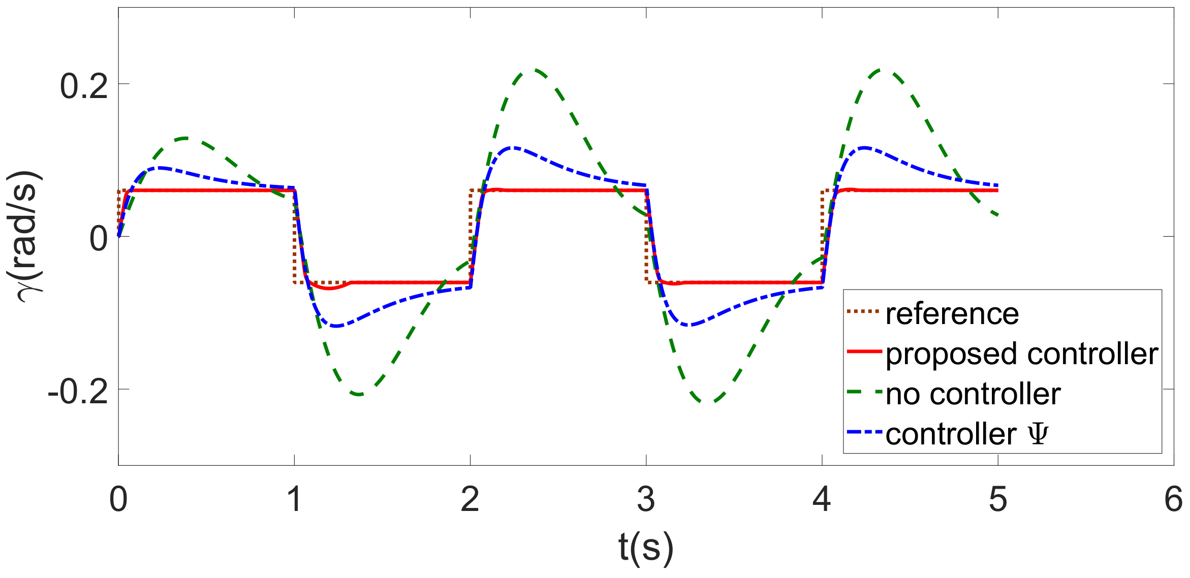
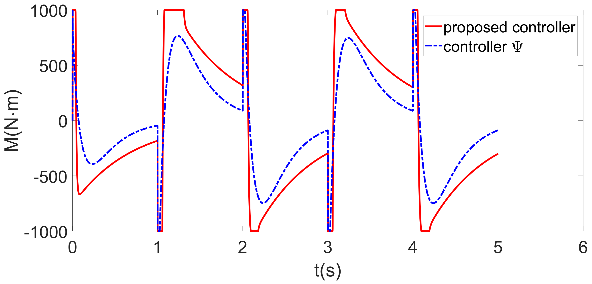
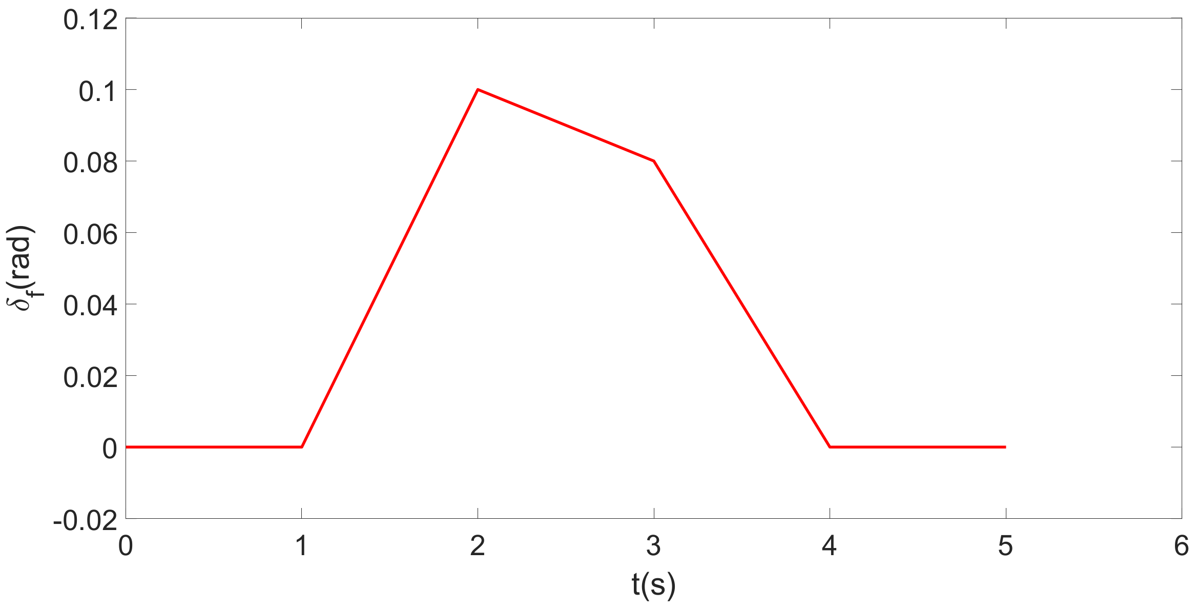
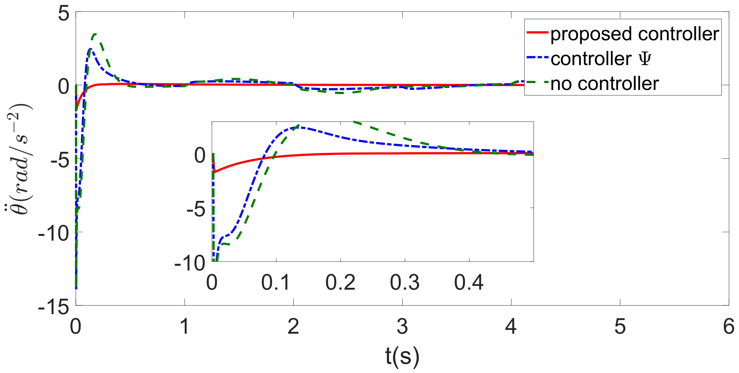
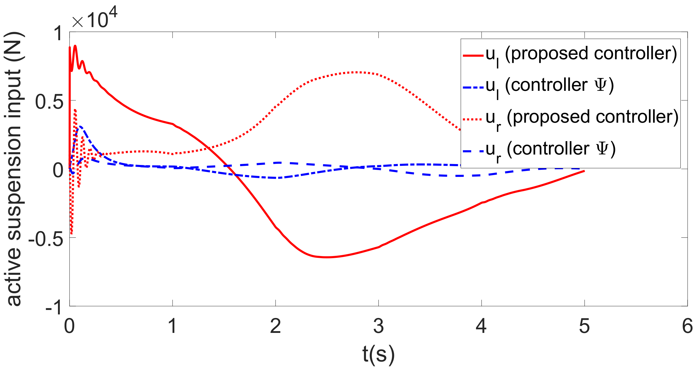
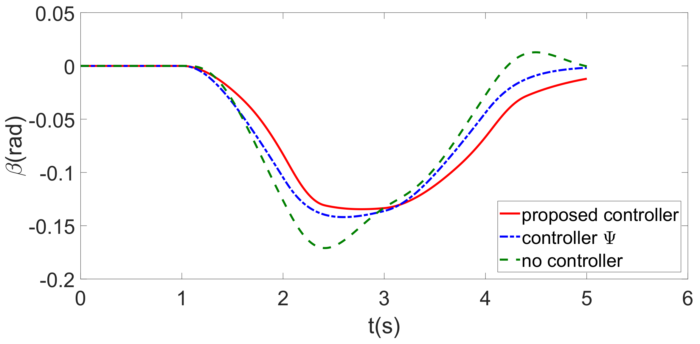
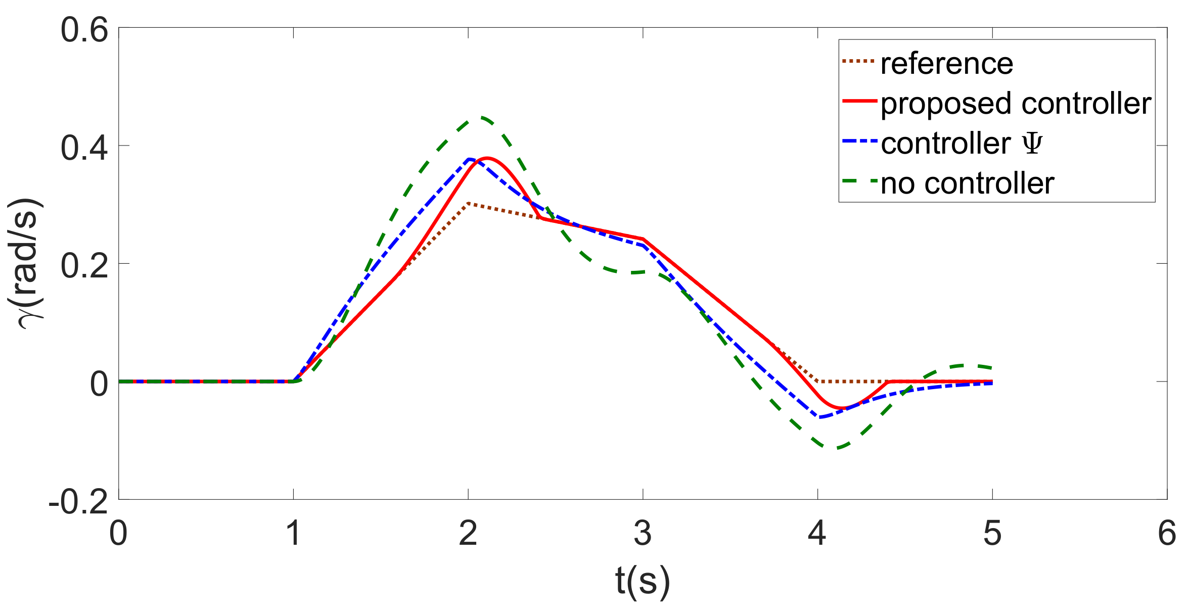
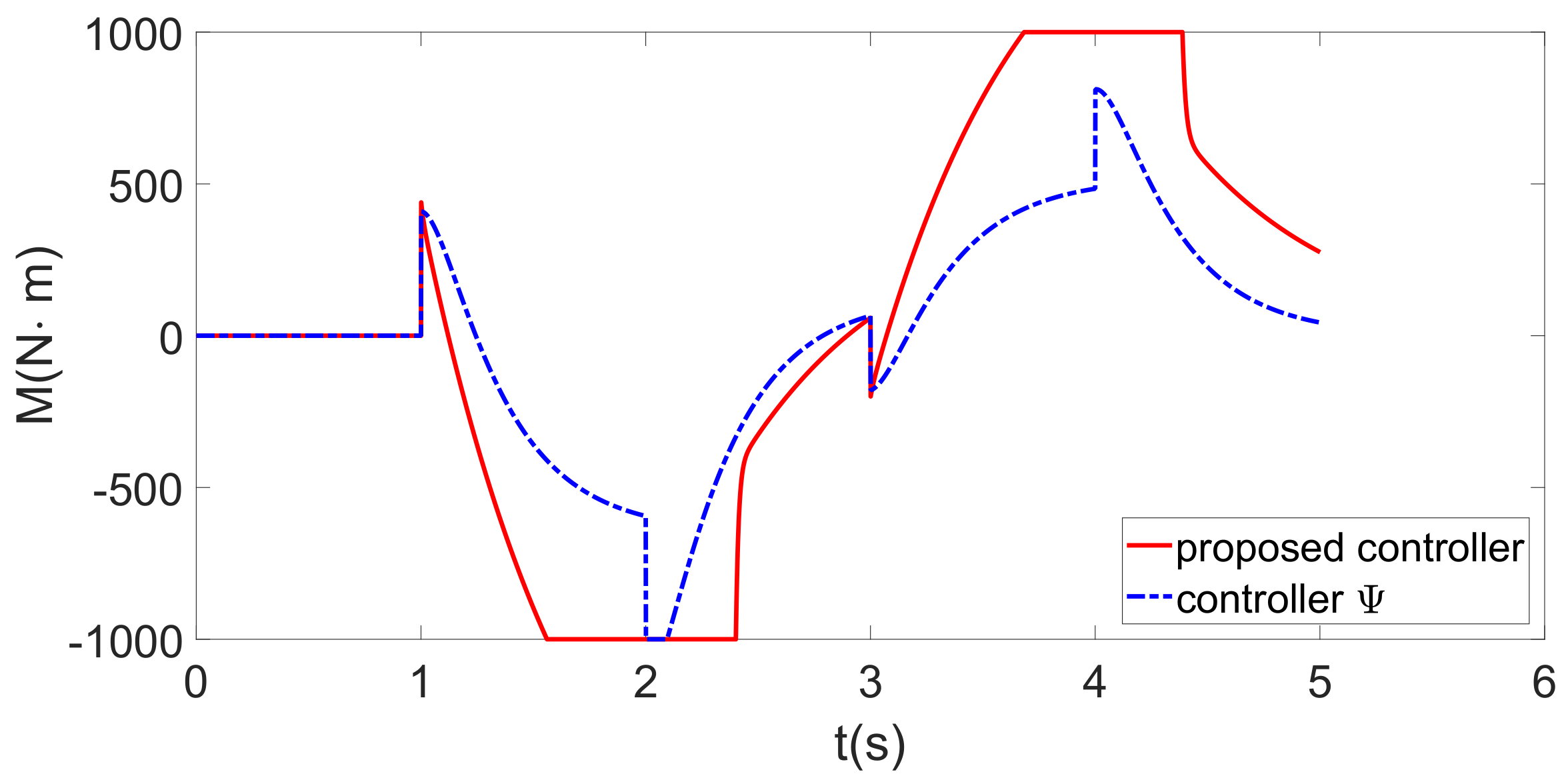
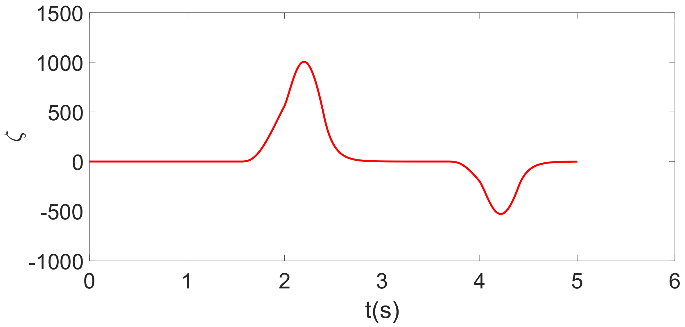
4.1. Scenario 1: Square-Wave Front Wheel Input with Flat Road Surface

In this scenario, the vehicle runs on a flat road under a square-wave front road wheel input with 0.5 Hz frequency and 0.01 rad amplitude. The simulation results are exhibited in Figure 3, Figure 4, Figure 5, Figure 6, Figure 7, Figure 8, Figure 9 and Figure 10.
The vehicle body vertical displacement and acceleration are illustrated in Figure 3 and Figure 4, respectively, from which it can be seen that the proposed controller can render the heave motion of the sprung mass as zero, asymptotically stable, and decrease the vertical acceleration dramatically, hence, improving vehicle ride comfort. Although the vertical displacement under the proposed controller converges slower than under the comparative controller Ψ , the vertical acceleration converges much faster, effectively improving ride comfort, as the vertical acceleration, rather than the displacement, is the main comfort index.
Figure 5 and Figure 6 exhibit the vehicle roll angle and roll angular acceleration. From Figure 5 and Figure 6, it can be seen that the roll motion can be stabilized using the proposed integrated controller, while controller Ψ can hardly realize it. The roll and heave control input, that is, the active suspension input force, is presented in Figure 7.
The vehicle sideslip angle and yaw rate are illustrated in Figure 8 and Figure 9, supposing that the maximum yaw control effort satisfies u m a x = 1000 N. Figure 9 indicates that lower performance degradation can be guaranteed with the proposed controller when saturation of the yaw control actuator occurs. In addition, Figure 8 shows that the vehicle under the proposed controller possesses a lower sideslip angle compared with respect to the compared controller, making for more stable lateral motion with the proposed controller.
The yaw motion control input is illustrated in Figure 10, and the corresponding state of the anti-windup compensator ζ is illustrated in Figure 11. From these two figures, it can be seen that when the control input reaches the actuator limitation u m a x , the state of the anti-windup compensator ζ accordingly increases its value such that the control input decreases by feeding ζ back into the control input u y , consequently reducing the impact of actuator saturation on control performance.

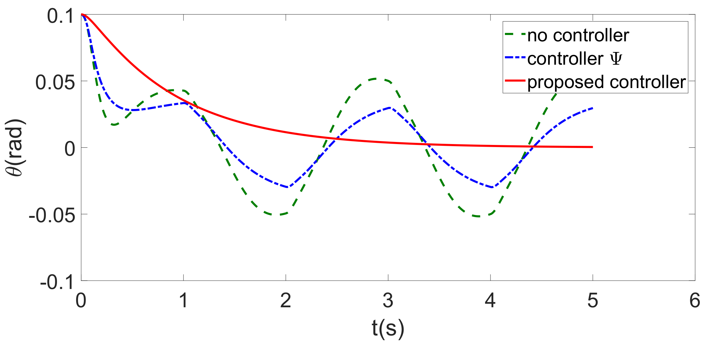
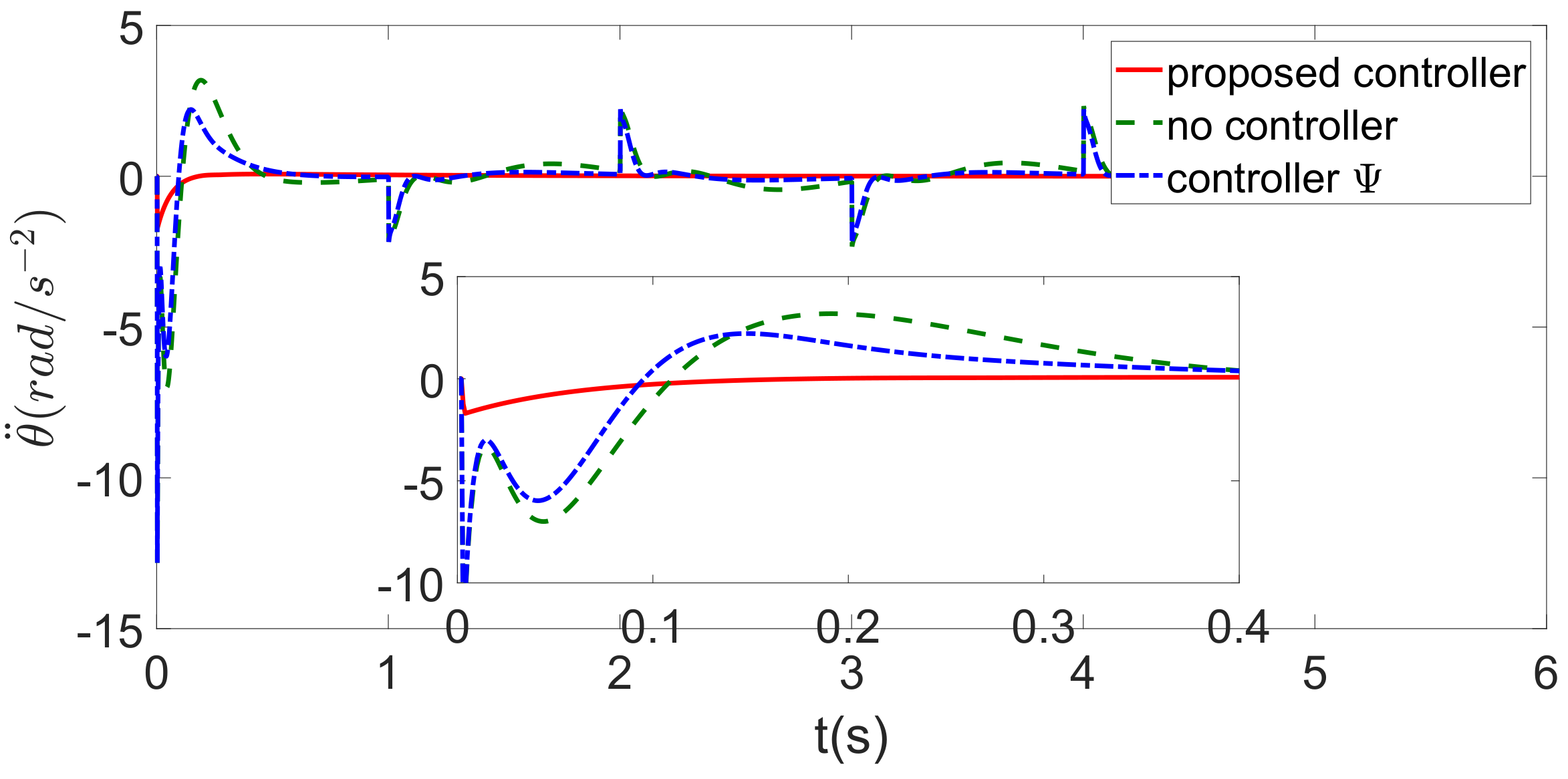
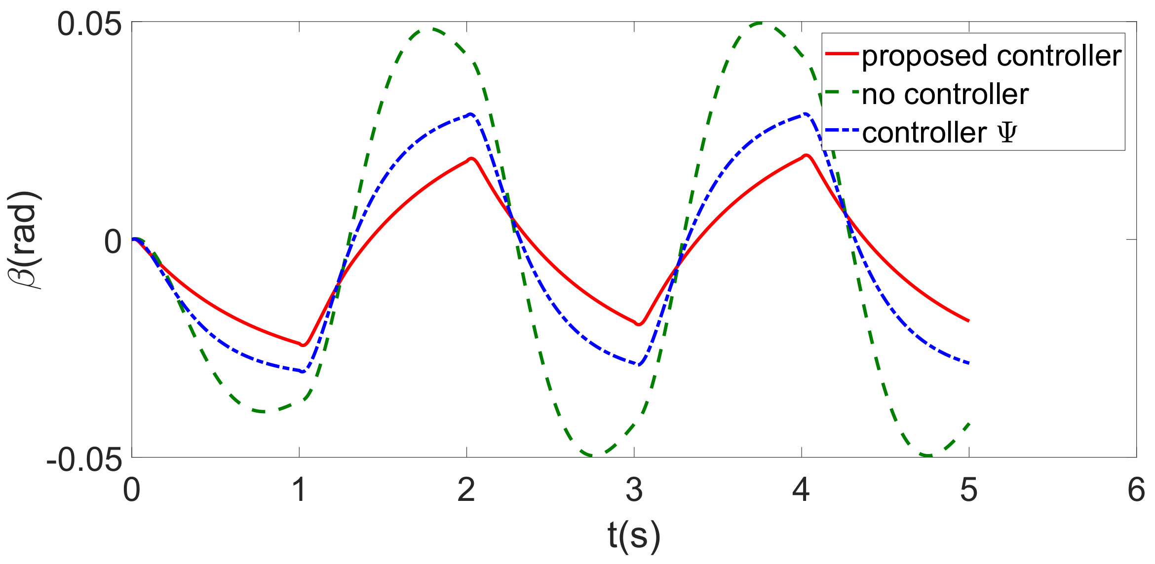
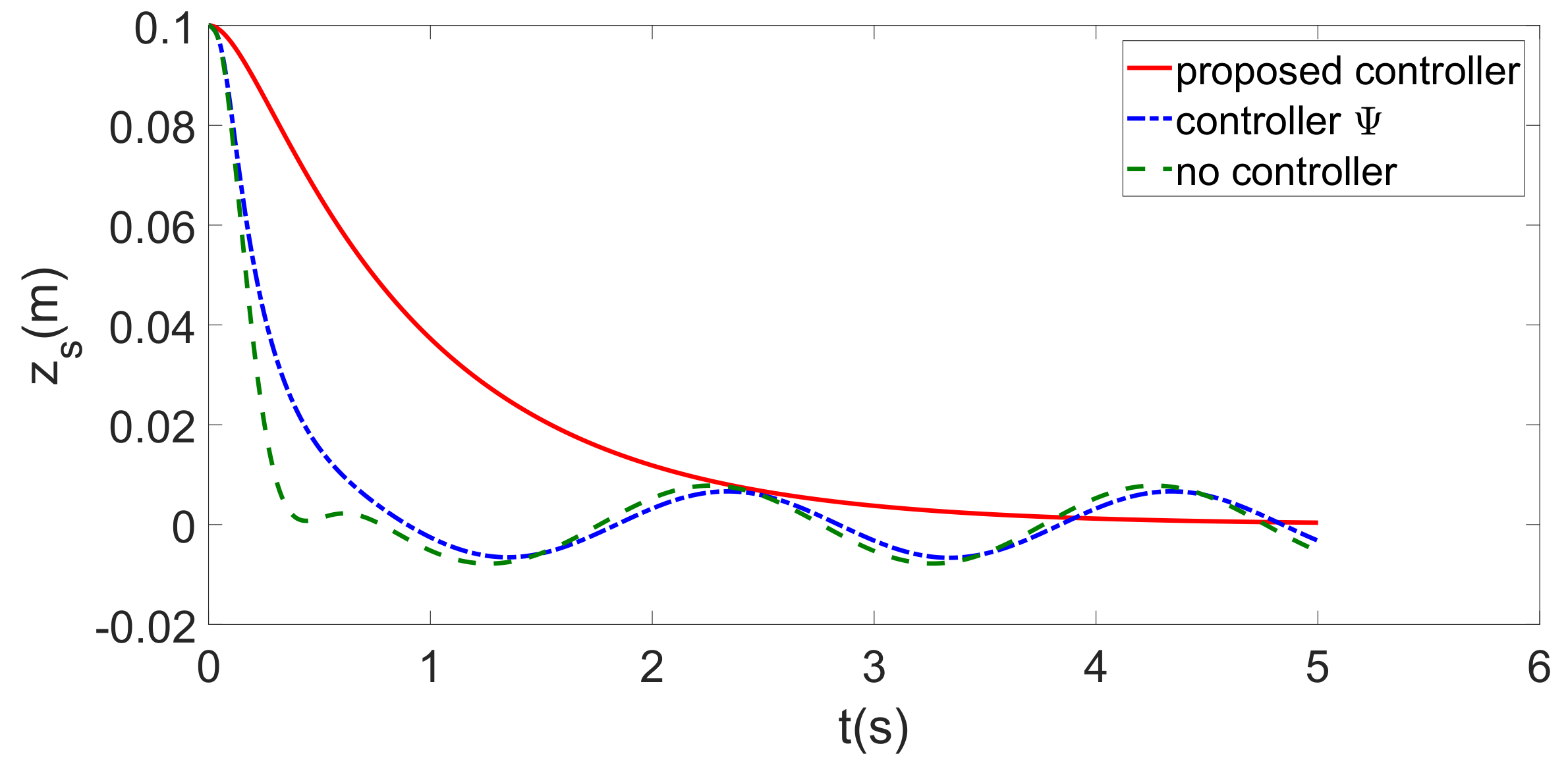
4.2. Scenario 2: J-Turn Front Wheel Input with Sinusoidal Vertical Road Surface

To further demonstrate the effectiveness of the proposed controller on steering stability under more severe circumstances, another scenario involving J-turn front wheel input and a sinusoidal vertical road surface was used as an additional simulation environment. The J-turn manoeuvre represents a type of sharp turning operation; the corresponding front wheel steering angle input is provided in Figure 12. The sinusoidal vertical road input is set as z r l = 0.01 s i n ( π t ) for the left wheel and z r r = 0.01 c o s ( π t ) for the right wheel. The controller parameters are kept identical to those in Section 4.1.
The simulation results are shown in Figure 13, Figure 14, Figure 15, Figure 16, Figure 17, Figure 18, Figure 19, Figure 20 and Figure 21. Figure 13, Figure 14, Figure 15, Figure 16 and Figure 17 show the sprung mass dynamics and the corresponding active suspension control inputs, while Figure 18 and Figure 19 show the the later motion dynamics. A detailed elaboration is not provided here due to the similarity between this scenario and the first scenario described in Section 4.1.
The yaw motion control input M together with the state of the anti-windup compensator ζ are shown in Figure 20 and Figure 21. Similarly, it can be seen that by feeding back ζ the controller saturation can be alleviated, thereby reducing the control impact from actuator saturation.
In short, the proposed controller can provide lower vehicle body vertical and roll angle acceleration, thus improving vehicle ride comfort, and simultaneously guaranteeing alleviation of yaw rate tracking performance degradation caused by actuator saturation.
It should be noted that the yaw rate is taken as the controlled state and the sideslip angle is not considered in the proposed controller. On the one hand, the zero dynamics of the sideslip angle is proven to be stable by Equation (18); on the other hand, from [38], we know that a small lateral velocity and sideslip angle can be maintained under the condition that yaw rate is controlled to track its reference value. Furthermore, the road condition is not considered in this paper; for pracitical implementation, the refence yaw rate can be replaced by
γ r = v v L L 1 + K v 2 δ f i f v v L L 1 + K v 2 δ f < μ g μ g v sgn ( v v L L 1 + K v 2 δ f ) o t h e r w i s e .

5. Conclusions

In this paper, an integrated vehicle dynamics under steering manoeuvre is established, initially considering the steering influence on the vehicle body roll motion; a corresponding integrated controller is then proposed. Our simulation results indicate that the proposed integrated controller can stabilize vehicle roll motion caused by steering and simultaneously alleviate vehicle yaw rate tracking performance degradation caused by yaw control actuator saturation. The implementation of the proposed controller will be the focus of our future research.

Author Contributions

Conceptualization, J.Z.; Data curation, J.Z.; Formal analysis, J.Z.; Funding acquisition, J.Z.; Investigation, M.W.; Methodology, M.W.; Project administration, M.W.; Resources, M.W. All authors have read and agreed to the published version of the manuscript.

Funding

This research was funded by the Guangzhou Science and Technology Plan Project (202201020173, 202201010475).

Institutional Review Board Statement

Not applicable.

Informed Consent Statement

Not applicable.

Data Availability Statement

Not applicable.

Conflicts of Interest

The authors declare no conflict of interest.

References

  1. Hu, J.; Wang, Y.; Fujimoto, H.; Hori, Y. Robust yaw stability control for in-wheel motor electric vehicles. IEEE/ASME Trans. Mechatron. 2017, 22, 1360–1370. [Google Scholar] [CrossRef]
  2. Sun, W.; Tang, S.; Gao, H.; Zhao, J. Two time-scale tracking control of nonholonomic wheeled mobile robots. IEEE Trans. Control Syst. Technol. 2016, 24, 2059–2069. [Google Scholar] [CrossRef]
  3. Choi, M.; Choi, S.B. Model predictive control for vehicle yaw stability with practical concerns. IEEE Trans. Veh. Technol. 2014, 63, 3539–3548. [Google Scholar] [CrossRef]
  4. Zhang, J.; Sun, W.; Du, H. Integrated motion control scheme for four-wheel-independent vehicles considering critical conditions. IEEE Trans. Veh. Technol. 2019, 68, 7488–7497. [Google Scholar] [CrossRef]
  5. Li, B.; Du, H.; Li, W.; Zhang, Y. Side-slip angle estimation based lateral dynamics control for omni-directional vehicles with optimal steering angle and traction/brake torque distribution. Mechatronics 2015, 30, 348–362. [Google Scholar] [CrossRef]
  6. Zhao, H.; Gao, B.; Ren, B.; Chen, H. Integrated control of in-wheelmotor electric vehicles using a triple-step nonlinear method. J. Frankl. Inst. 2015, 352, 519–540. [Google Scholar] [CrossRef]
  7. Pugi, L.; Favilli, T.; Berzi, L.; Cappa, M.; Pierini, M. An Optimal Torque and Steering Allocation Strategy for Stability Control of Road Vehicles. In Proceedings of the 21st IEEE International Conference on Environment and Electrical Engineering and 2021 5th IEEE Industrial and Commercial Power System Europe, EEEIC/I and CPS Europe 2021—Proceedings, Bari, Italy, 7–10 September 2021. [Google Scholar]
  8. Allotta, B.; Pugi, L.; Bartolini, F.; Cangioli, F.; Colla, V. Comparison of different control approaches aiming at enhancing the comfort of a railway vehicle. In Proceedings of the IEEE/ASME International Conference on Advanced Intelligent Mechatronics, Montreal, QC, Canada, 6–9 July 2010; pp. 676–681. [Google Scholar]
  9. Cairano, S.D.; Tseng, H.E.; Bernardini, D.; Bemporad, A. Vehicle yaw stability control by coordinated active front steering and differential braking in the tire sideslip angles domain. IEEE Trans. Control Syst. Technol. 2017, 21, 1236–1248. [Google Scholar] [CrossRef]
  10. Sun, W.; Pan, H.; Gao, H. Filter-based adaptive vibration control for active vehicle suspensions with electro-hydraulic actuators. IEEE Trans. Veh. Technol. 2016, 65, 4619–4626. [Google Scholar] [CrossRef]
  11. Zhang, J.; Sun, W.; Liu, Z.; Zeng, M. Comfort braking control for brake-by-wire vehicles. Mech. Syst. Signal Process. 2019, 133, 106255. [Google Scholar] [CrossRef]
  12. Zhang, J.; Sun, W.; Jing, H. Nonlinear Robust Control of Antilock Braking Systems Assisted by Active Suspensions for Automobile. IEEE Trans. Control Syst. Technol. 2019, 27, 1352–1359. [Google Scholar] [CrossRef]
  13. Sun, W.; Pan, H.; Zhang, Y.; Gao, H. Multi-objective control for uncertain nonlinear active suspension systems. Mechtronics 2014, 24, 318–327. [Google Scholar] [CrossRef]
  14. Sun, W.; Gao, H.; Yao, B. Adaptive robust vibration control of full-car active suspensions with electrohydraulic actuators. IEEE Trans. Control Syst. Technol. 2013, 21, 2417–2422. [Google Scholar] [CrossRef]
  15. Riofrio, A.; Sanz, S.; Boada, M.J.L.; Boada, B.L. A lqr-based controller with estimation of road bank for improving vehicle lateral and rollover stability via active suspension. Sensors 2017, 17, 2318. [Google Scholar] [CrossRef]
  16. Her, H.; Suh, J.; Yi, K. Integrated control of the differential braking, the suspension damping force and the active roll moment for improvement in the agility and the stability. Proc. Inst. Mech. Eng. Part D J. Automob. Eng. 2015, 229, 1145–1157. [Google Scholar] [CrossRef]
  17. Chou, H.; D’andréa-Novel, B. Global vehicle control using differential braking torques and active suspension forces. Veh. Syst. Dyn. 2005, 43, 261–284. [Google Scholar] [CrossRef]
  18. Cao, J.; Jing, L.; Guo, K.; Yu, F. Study on integrated control of vehicle yaw and rollover stability using nonlinear prediction model. Math. Probl. Eng. 2013, 2013, 643548. [Google Scholar] [CrossRef]
  19. Hsin, G.; Kyongil, K.; Wang, B. Comprehensive path and attitude control of articulated vehicles for varying vehicle conditions. Int. J. Heavy Veh. Syst. 2017, 24, 65–95. [Google Scholar]
  20. Saeedi, M.A. A new robust combined control system for improving manoeuvrability, lateral stability and rollover prevention of a vehicle. Proc. Inst. Mech. Eng. Part K J. Multi-Body Dyn. 2020, 1, 198–213. [Google Scholar] [CrossRef]
  21. Williams, D.E.; Haddad, W.M. Nonlinear control of roll moment distribution to influence vehicle yaw characteristics. IEEE Trans. Control Syst. Technol. 1995, 3, 110–116. [Google Scholar] [CrossRef]
  22. Sun, W.; Zhao, Z.; Gao, H. Saturated adaptive robust control for active suspension systems. IEEE Trans. Ind. Electron. 2013, 60, 3889–3896. [Google Scholar] [CrossRef]
  23. Hong, Y.; Yao, B. A globally stable high-performance adaptive robust control algorithm with input saturation for precision motion control of linear motor drive systems. IEEE/ASME Trans. Mechatron. 2007, 12, 198–207. [Google Scholar] [CrossRef]
  24. Tarbouriech, S.; Turner, M. Anti-windup design: An overview of some recent advances and open problems. IET Control Theory Appl. 2009, 3, 1–19. [Google Scholar] [CrossRef]
  25. Wen, C.; Zhou, J.; Liu, Z.; Su, H. Robust adaptive control of uncertain nonlinear systems in the presence of input saturation and external disturbance. IEEE Trans. Autom. Control 2011, 56, 1672–1678. [Google Scholar] [CrossRef]
  26. Sun, L.; Zheng, Z. Disturbance-observer-based robust backstepping attitude stabilization of spacecraft under input saturation and measurement uncertainty. IEEE Trans. Ind. Electron. 2017, 64, 7994–8002. [Google Scholar] [CrossRef]
  27. Wang, F.; Zou, Q.; Zong, Q. Robust adaptive backstepping control for an uncertain nonlinear system with input constraint based on lyapunov redesign. Int. J. Control Autom. Syst. 2017, 15, 212–225. [Google Scholar] [CrossRef]
  28. Zhang, J.; Sun, W.; Feng, Z. Vehicle yaw stability control via H gain scheduling. Mech. Syst. Signal Process. 2018, 106, 62–75. [Google Scholar] [CrossRef]
  29. Yao, J.; Deng, W.; Jiao, Z. Adaptive control of hydraulic actuators with LuGre model based friction compensation. IEEE Trans. Ind. Electron. 2015, 62, 6469–6477. [Google Scholar] [CrossRef]
  30. Sun, W.; Zhang, Y.; Huang, Y.; Gao, H.; Kaynak, O. Transient-performance-guaranteed robust adaptive control and its application to precision motion control systems. IEEE Trans. Ind. Electron. 2016, 63, 6510–6518. [Google Scholar] [CrossRef]
  31. Chen, Z.; Yao, B.; Wang, Q. μ-synthesis based adaptive robust control of linear motor driven stages with high-frequency dynamics: A case study with comparative experiments. IEEE/ASME Trans. Mechatron. 2015, 20, 1482–1490. [Google Scholar] [CrossRef]
  32. Zhang, H.; Huang, X.; Wang, J.; Karimi, H.R. Robust energy-to-peak sideslip angle estimation with applications to ground vehicles. Mechatronics 2015, 30, 338–347. [Google Scholar] [CrossRef]
  33. Yi, J. A piezo-sensor-based “smart tire” system for mobile robots and vehicles. IEEE/ASME Trans. Mechatron. 2008, 13, 95–103. [Google Scholar] [CrossRef]
  34. Cheli, F.; Leo, E.; Melzi, S.; Sabbioni, E. On the impact of ‘smart tyres’ on existing ABS/EBD control systems. Veh. Syst. Dyn. 2010, 48, 255–270. [Google Scholar] [CrossRef]
  35. Wang, R.; Wang, J. Actuator-redundancy-based fault diagnosis for four-wheel independently actuated electric vehicles. IEEE Trans. Intell. Transp. Syst. 2014, 15, 239–249. [Google Scholar] [CrossRef]
  36. Wei, X.; Wu, Z.; Karimi, H.R. Disturbance observer-based disturbance attenuation control for a class of stochastic systems. Automatica 2016, 63, 21–25. [Google Scholar] [CrossRef]
  37. Wang, R.; Wang, J. Fault-tolerant control for electric ground vehicles with independently-actuated in-wheel motors. J. Dyn. Syst. Meas. Control 2012, 134, 021014. [Google Scholar] [CrossRef]
  38. Zhou, H.; Liu, Z. Vehicle yaw stability-control system design based on sliding mode and backstepping control approach. IEEE Trans. Veh. Technol. 2010, 59, 3674–3678. [Google Scholar] [CrossRef]
Figure 1. Vehicle model.
Applsci 12 08502 g001
Figure 2. Control scheme flowchart.
Applsci 12 08502 g002
Figure 3. Vehicle body vertical displacement.
Applsci 12 08502 g003
Figure 4. Vehicle body vertical acceleration.
Applsci 12 08502 g004
Figure 5. Vehicle roll angle.
Applsci 12 08502 g005
Figure 6. Vehicle roll angular acceleration.
Applsci 12 08502 g006
Figure 7. Active suspension input.
Applsci 12 08502 g007
Figure 8. Vehicle sideslip angle.
Applsci 12 08502 g008
Figure 9. Vehicle yaw rate.
Applsci 12 08502 g009
Figure 10. Yaw motion control input.
Applsci 12 08502 g010
Figure 11. State of the anti-windup compensator.
Applsci 12 08502 g011
Figure 12. Front wheel input for J-turn simulation.
Applsci 12 08502 g012
Figure 13. Vehicle body vertical displacement.
Applsci 12 08502 g013
Figure 14. Vehicle body vertical acceleration.
Applsci 12 08502 g014
Figure 15. Vehicle roll angle.
Applsci 12 08502 g015
Figure 16. Vehicle roll angular acceleration.
Applsci 12 08502 g016
Figure 17. Active suspension input.
Applsci 12 08502 g017
Figure 18. Vehicle sideslip angle.
Applsci 12 08502 g018
Figure 19. Vehicle yaw rate.
Applsci 12 08502 g019
Figure 20. Yaw moment control input.
Applsci 12 08502 g020
Figure 21. State of the anti-windup compensator.
Applsci 12 08502 g021
Table 1. Parameters of the vehicle model.
ParameterValueParameterValue
m s 1110 kg m w 2 × 30 kg
I x 440.6 kg·m 2 I z 1343.1 kg·m 2
c s 2 × 4000 Ns/m k s 2 × 28,000 N/m
c w 2 × 1000 Ns/m k w 2 × 232,000 N/m
c f 22,010 N/rad c r 22,010 N/rad
h g 0.54 md 0.74 m
a 1.04 mb 1.56 m
θ I m a x 1 / 400 kg 1 ·m 2 θ I m i n 1 / 600 kg 1 ·m 2
Table 2. Parameters of the proposed controller and the compared controller.
ParameterValueParameterValueParameterValue
k 1 1 k 2 10,000 k 3 10
k 4 1 k 10 100 k ζ 10
r 0 10 σ 0.01 r 1 5000
r 2 0.001 k 11 0.1 k γ , k θ , k z 10
Publisher’s Note: MDPI stays neutral with regard to jurisdictional claims in published maps and institutional affiliations.

