Experimental Study on Interface Model of Asphalt Pavement under Vertical Load

Abstract

Layered asphalt pavement makes the interlayer contact more complicated. In order to further understand the characteristics of interlayer interface of asphalt pavement under vehicle load, this paper analyzes the change rule of interlayer interface of asphalt pavement under a vertical load condition, based on the Goodman model. According to the characteristics of asphalt pavement, the experiment temperature, gradation, amount of viscosity-level oil, type of viscosity-level oil, and vertical compressive stress are taken as parameters, and the universal testing machine (UTM) and self-modified test fixture are used to carry out the direct interlayer shear test. Experimental results show that the vertical load has a significant effect on the characteristics of the interlayer interface. With an increase in the vertical load, the maximum bonding coefficient changes greatly. Additionally, when the vertical load is constant, the temperature and spreading amount of viscosity-level oil have a strong influence on the interlayer bonding state. With an increase in temperature, the maximum bonding coefficient decreases. The adhesion coefficient increases first and then decreases with increasing spreading amount. The best spreading amounts of oil between the upper and middle layers, the middle and lower layers, and the lower layer and cement-stabilized base layer under different vertical load conditions are recommended. This study offers important guidance for designing pavement structure.

1. Introduction

It is known that the existing structural design theory of asphalt pavement is mainly based on the multilayer elastic system theory, and the interlayer interface is assumed to be completely continuous or completely smooth [1,2]. Certainly, each country has its own design criteria and specifications for road design. In China, based on Specifications for Design of Highway Asphalt Pavement [3], the pavement structure is also considered as a layered elastic continuous system to solve the interlayer contact problem of asphalt pavement. Additionally, a further regulation on the construction between layers is proposed in Technical Specification for construction of Highway Asphalt Pavement [4] to make the actual working state of the asphalt pavement conform to the ideal state as much as possible. The asphalt mixture layer, semirigid base layer, and structural layer of each asphalt mixture are closely combined into a whole. However, asphalt pavement is layered and rolled in layers, which leads to the fact that the contact between layers cannot be completely continuous [5]. In addition, owing to the structural depth of the surface, the surface texture of aggregate and the adhesion between asphalt films, the interlayer contact cannot be completely smooth [6]. Therefore, it is not accurate to simply regard each structural layer of asphalt pavement as completely continuous or completely smooth.

To improve the understanding of the interlayer interface model, avoid the early interlayer slip failure, and establish a set of standards for evaluating the bond ability of asphalt pavement, some researchers have done much work through software modeling calculation and laboratory experiments. In 1962, the research results of Livneh and Shklarsky [7] showed that the interlayer interface would cause crescent-shaped or semicrescent-shaped slip cracks, which had a serious impact on pavement performance. Immediately, extensive research on the problem of interlayer bonding was performed, and many interlayer interface models were also put forward to analyze the reasons for interlayer diseases. Among them, the Goodman model is the most widely used.

In 1968, the famous Goodman model was put forward by Goodman and Brekke [8] to solve the contact problem of jointed rock. They found that the interlayer shear stress is proportional to interlayer relative displacement. With continuous optimization of the Goodman model, it has become the first choice for researchers to study interlayer interface problems. Based on the Goodman model and by numerical simulation and direct shear test, Uzan et al. [9] analyzed and calculated the stress and strain of pavement structure with the change in the interlayer bond coefficient. The results showed that the interlayer shear strength decreases with the decrease in vertical compressive stress or the increase in temperature when the interlayer adhesion coefficient is 10⁸~10¹² N/m³, and the interlayer shear strength reaches a maximum when the amount of adhesive oil is in an optimal range. Romanoschi and Metcalf [10] described the interlayer interface behavior through interlayer reaction modulus, shear strength, and friction coefficient after instability. In addition, Mariana et al. [11] studied the interlayer stiffness of different interlayer bonding materials, and believed that the material of double-layer structure has a greater impact on interlayer bonding strength than that of interlayer bonding material, and the interface bonding between the base and subgrade had the most adverse impact on pavement life. Leng et al. [12] found that the type and temperature of hot mix asphalt mixture has a strong influence on the interlayer bond strength, and there is an optimal oil spread rate of viscosity-level. However, Kruntcheva et al. [13] hold the opposite view that the adhesive material of interlayer interface has more influence than the amount of spread and interface conditions (roughness, etc.). Hu and Walubita [14] showed that the failure of pavement is directly related to the quality of interlayer bonding. The interlayer bonding has obvious influence on the stress, strain, and displacement of pavement structure. If interlayer separation occurs, obviously, the transverse and longitudinal tensile strains of asphalt pavement layer will increase.

To summarize, research concerning the simulation of pavement and interlayer contact is insufficient. Extensive research on interlayer stress and theoretical models has been performed, but some issues remain unsolved. For example, the study of interlayer interface based on numerical simulation only considers the friction between layers, and the intercalation between aggregates, which inevitably affects the mechanical response of the pavement structure, has not been considered. Additionally, the effect of vertical load on the stress state of the interlayer interface is rarely considered when interlayer shear molds are developed. Even if considered, the vertical load is a constant simulation value, which is far from the actual value. The interfacial characteristics of asphalt layers under different vertical load conditions, different spraying amounts, and different temperatures are also rarely studied. Therefore, it is necessary to perform research on different types of interlayer contact under vertical load.

In view of the above, this paper describes an investigation of varying the interlayer interface of asphalt pavement under the condition of a vertical load, based on Goodman’s model. The experiment temperature, gradation, amount of viscosity-level oil, type of viscosity-level oil, and vertical compressive stress are chosen as the main test parameters, and interlayer direct shear tests are conducted using a universal testing machine (UTM) and self-modified test fixture. Based on the experimental and theoretical analysis, the basic variation rules of the interlayer characteristics of the mixture under different conditions are obtained. Additionally, the optimal spraying amounts of the interlayer viscous oil between the upper and middle layers, the middle and lower layers, the lower layer and the cement-stabilized base layer are recommended.

2. Test Equipment and Material Properties

2.1. Introduction of the Equipment

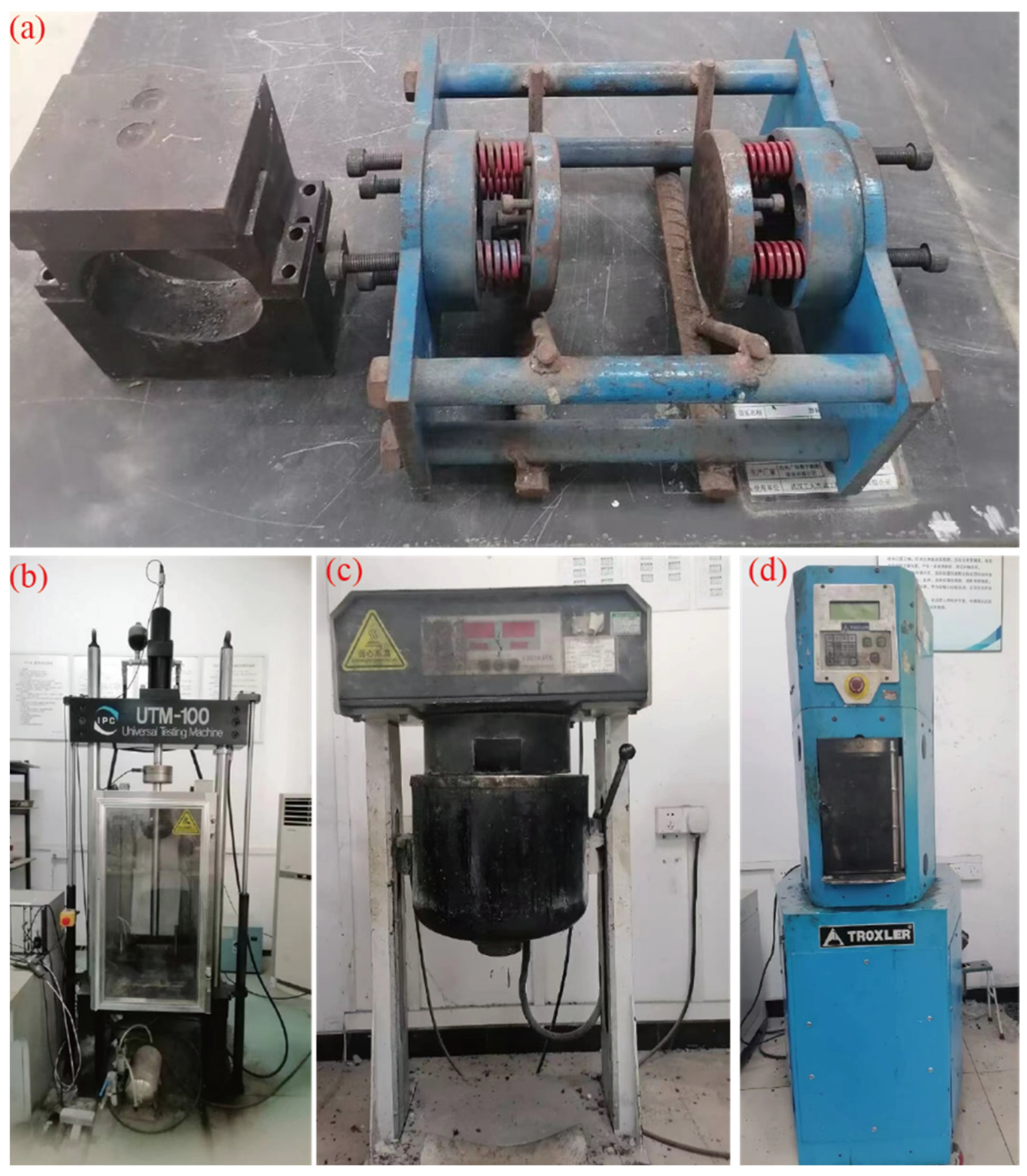
The main instruments used in this experiment include: the self-modified test fixture that can be used to apply vertical force, the hydraulic servo multifunctional material testing machine UTM-100, the asphalt mixture mixer, and SGC (Superpave Gyratory Compactor), as shown in Figure 1.

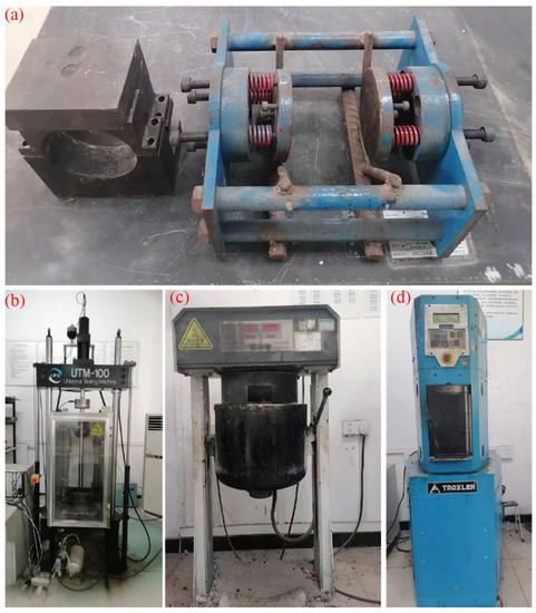
Figure 1. Experimental equipment: (a) a shear test fixture for applying vertical force; (b) multifunction testing machine UTM-100; (c) asphalt mixture mixer; (d) SGC (Superpave Gyratory Compactor).

In this study, UTM-100 is mainly used to apply shear force to specimens. During the test, some of the specimens are in an environment chamber where the temperature and load can be precisely controlled. The main technical parameters of UTM-100 are shown in Table 1.

Table 1. The main technical parameters of UTM-100.

Technical Indicators	Unit	Value or Range
Test temperature range	°C	−20~80
Maximum vertical load	kN	100
Pressure sensor accuracy	kN	0.01
Displacement sensitivity	mm	0.001
Loading rate	Adjustable
Data acquisition	Automatic

2.2. Test Parameters

The contact state of the interlayer interface is related to the type and gradation of upper- and lower-layer materials, the type and number of adhesive materials, test temperature, specimen size, shear rate, and other factors. The test parameters were selected as follows.

Test temperature: According to the climatic characteristics, −10, 0, 25, and 50 °C were selected as the test temperatures which reflect the asphalt mixture temperature of pavement under the conditions of low temperature, 0 degrees, room temperature, and high temperature.

Mixture type: According to the characteristics of mixture types commonly used for asphalt pavement and cement-stabilized base, three kinds of asphalt mixture (AC-13, AC-20, and AC-25) and one kind of cement-stabilized base mixture were adopted.

Specimen size: Referring to relevant data, the stability of the shear test data has a certain relationship with the size of the specimen. The data obtained from specimens with larger size indicate more stability than smaller size specimens. According to existing research results [15], a specimen diameter of 100 mm is relatively stable. Therefore, the 100 mm diameter was taken as the basic size of the specimen used in this study, and the thickness of the asphalt mixture specimen was 50 mm.

The amount of viscosity-level oil spread: According to the amount and type of viscosity-level oil used in asphalt pavement construction, two different viscosity-level oil types were considered in this study, namely, PC-3 fast-cracking cationic emulsified asphalt and high viscosity fast-cracking cationic emulsified asphalt. Three different densities of emulsified asphalt were selected, namely, 0.5, 1.0, 1.5 kg/m².

Vertical compressive stress: Combined with mechanical calculation, 0.7 MPa was selected as the vertical compressive stress between the AC-13 and AC-20 layers; 0.16 MPa was selected as the vertical compressive stress between the AC-20 and AC-25 layers; and 0.07 MPa was selected as the vertical compressive stress between AC-25 and the cement-stabilized base layer, striving to be closer to the actual stress of each structural layer on the road surface.

Shear rate: Based on existing research results [16], a shear rate of 5 mm/min was selected for the test.

2.3. Test of Material Performance

(1)

Performance of asphalt binder material

The base asphalt used was SK70# road petroleum asphalt, which conforms to the Technical Specification for Construction of Highway Asphalt Pavement JTG F40-2004 [4]. The technical specifications are shown in Table 2. The technical indexes of the two cationic emulsified asphalts are shown in Table 3 and Table 4.

Table 2. Test results of asphalt raw materials.

Test Items	Measured Data AH-70	Technical Requirements AH-70	Test Method
Penetration (25 °C, 100 g, 5 s, 0.1 mm)	79.4	60~80	T0604
Softening point (°C)	46.76	≥46	T0606
Ductility (10 °C) (cm)	147.5	≥20	T0605
Ductility (15 °C) (cm)	>200	≥100
60 °C Dynamic viscosity (Pa.s)	297	≥180	T0620
Asphalt flash point (°C)	284	≥46	T0611
Residual needle penetration ratio (25 °C)	82.1	≥61	T0604
Residual ductility (10 °C) (cm)	8.5	≥6	T0605
Residual ductility (15 °C) (cm)	33	≥15	T0605

Table 3. Test results of emulsified asphalt A raw material.

Technical Indicators		Unit	Inspection Results	Test Method
Demulsification velocity		-	Quick to crack	T0658
Particle charge		-	Cationic (+)	T0653
On-screen residue (1.18 mm)		%	0.08	T0652
Viscosity	Engler viscometer	-	3	T0622
	Road standard viscometer	s	12	T0621
Evaporation residue	Evaporation residue content	%	59.4	T0651
	Penetration (25 °C)	0.1 mm	138.19	T0604
	Ductility (15 °C)	cm	126.67	T0605
	Solubility	%	99.4	T0607
Adhesion with coarse aggregate, adhesion area		-	≥2/3	T0654
Storage stability at room temperature	1 d	%	0.4	T0655
	5 d	%	1.8

Table 4. Test results of emulsified asphalt B raw material.

Technical Indicators		Unit	Inspection Results	Test Method
Demulsification velocity		-	Slow to crack	T0658
Particle charge		-	Cationic (+)	T0653
On-screen residue (1.18 mm)		%	0.07	T0652
Viscosity	Engler viscometer	-	3	T0622
	Road standard viscometer	s	14	T0621
Evaporation residue	Evaporation residue content	%	64.1	T0651
	Penetration (25 °C)	0.1 mm	57.0	T0604
	Ductility (15 °C)	cm	82.8	T0605
	Solubility	%	99.6	T0607
Adhesion with coarse aggregate, adhesion area		-	≥2/3	T 0654
Storage stability at room temperature	1 d	%	0.6	T0655
	5 d	%	2.0

(2)

Performance of the aggregate

According to the corresponding technical specifications, the aggregate selected should be clean, dry, exhibit a rough surface, and consist of hard quality stone. The test results of the main mechanical indexes are shown in Table 5 and Table 6.

Table 5. Coarse aggregate for asphalt mixture.

Index	Unit	Measured Value	Technical Requirement	Test Method
Crushing value of stone	%	20.4	≤26	T0316
Los Angeles attrition loss	%	25.33	≤28	T0317
Apparent relative density	%	2.855	≥2.60	T0304
Bibulous rate	%	0.68	≤2.0	T0304
Needle-like particle content	%	-	≤15	T0317
Water washing method <0.075 mm Particle concentration	%	0.93	≤1	T0310

Table 6. Fine aggregate for asphalt mixture.

Index		Unit	Measured Value	Technical Requirement	Test Method
Apparent relative density		t/m	2.625	≥2.5	T0328
Silt content		%	2.8	≤3.0	T0340
Sand equivalent		%	68.8	≥60	T0333
Angularity	AC-13 AC-20	s	45	≥30	T0345
		s	38

2.4. Set of Mixture

In this experiment, three asphalt mixture surface materials and a cement-stabilized gravel base material were used in the upper, middle, lower layers and cement-stabilized base of pavement structure, respectively. The selection of asphalt concrete at all levels is shown in Table 7, and the asphalt–stone ratios were 4.7%, 4.1%, and 3.8%, respectively. The sample of the cement-stabilized gravel layer was ground to the required height after drilling and retrieving a core sample from the construction site. It is worth noting that the horizontal interlayer shear action under vertical load was applied mainly to the specimen. This is a simplification of the actual engineering, and not exactly identical.

Table 7. Gradation of the selected asphalt mixture.

Mass Percentage through the Square Hole Screen
Specifications	26.5	19	16	13.2	9.5	4.75	2.36	1.18	0.6	0.3	0.15	0.075
AC-13	100	100	99.7	95.1	76.8	38.4	29.1	23.0	17.3	12.2	10.4	7.9
AC-20	100	99.1	91.1	73.3	54.9	30.3	23.6	18.7	14.2	10.0	8.6	6.6
AC-25	99.1	79.0	73.0	65.7	52.7	36.7	32.0	23.7	15.0	10.2	8.2	6.8

3.1. Interlayer Interface Model

(1)

Theoretical model

Under vehicle load, there is not only friction resistance but also relative horizontal displacement on the interlayer contact surface. The Goodman model is used in classical pavement mechanics to measure the mechanical state of interlayer bonding, as shown in Figure 2. When the relative horizontal displacement of the upper and lower layers of the interlayer interface is $\Delta u$, the shear stress can be expressed as Equation (1):

$$\tau =K\Delta u$$

(1)

where $K$ is the interlayer bonding coefficient (N/cm³), $\tau$ is the shear stress at the interlayer interface (N/cm²), and $\Delta u$ is the relative displacement at the interlayer interface (cm).

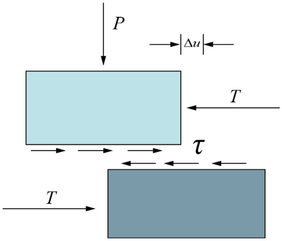
Figure 2. Goodman mechanical model.

After introducing the Goodman model, the contact conditions between arbitrary i-layers of multilayer elastomers are shown in Equation (2):

$${\tau }_{Zri}={\tau }_{Zri+1}=K_i(u_{i+1}-u_i)$$

(2)

where ${\tau }_{Zri}$, ${\tau }_{Zri+1}$ are the shear stresses (N/cm²) between the upper and lower layers of the i-th interlayer interface; $u_i$, $u_{i+1}$ are the displacement values of the upper and lower layers at the same point (cm); and $K_i$ is the i-layer bonding coefficient (N/cm³).

According to Equation (1), the value of the shear stress at the interface is the value of the interlayer bonding coefficient when unit-relative displacement occurs. The larger the value of the interlayer bonding coefficient, the better the adhesion between layers, and the more it tends to be completely continuous. Therefore, it is reasonable and feasible to evaluate the interlayer bonding state of the pavement by using the interlayer adhesion coefficient according to the Goodman model. By determining the average shear stress at the interlayer interface and the relative horizontal displacement at this stress value, the value of the interlayer bonding coefficient can be measured and the interlayer bonding state of the pavement can be evaluated.

(2)

Experimental model

The curve of the relationship between shear load and relative horizontal displacement at the interlayer interface of specimens is shown in Figure 3. The relationship curve between the interlayer bond coefficient K and the relative horizontal displacement is shown in Figure 4.

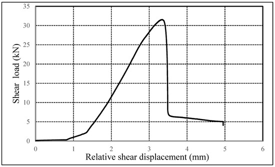
Figure 3. The relationship between interlayer shear load and relative shear displacement.

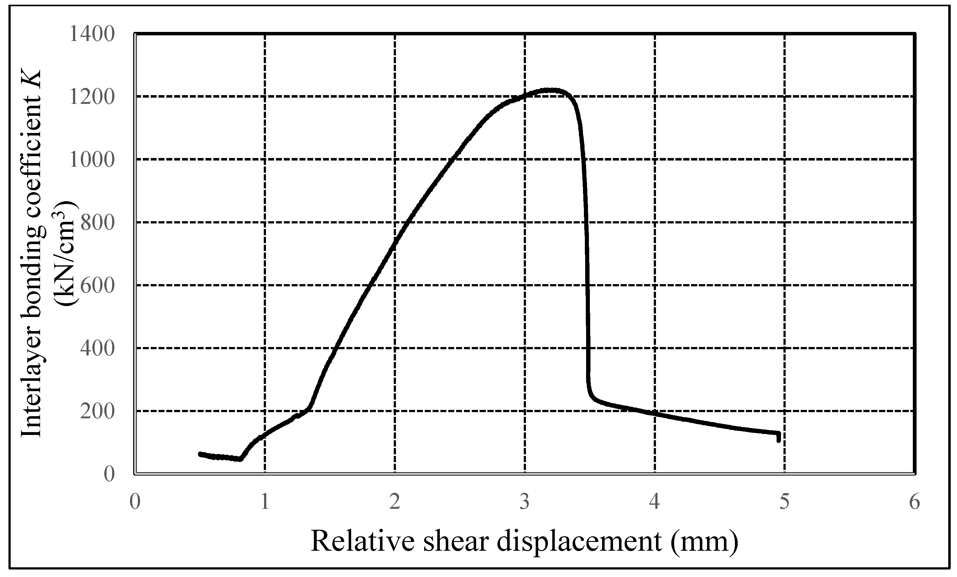
Figure 4. The relationship between interlayer bonding coefficient and relative shear displacement.

It can be seen from Figure 3 that with the increase in relative shear displacement, the shear load on the interlayer interface increases at first, and then decreases gradually to a stable state. According to this phenomenon, we can know that when the interlaminar shear load increases to the ultimate shear strength of the specimen, the interlayer structure is damaged. However, residual shear strength still exists between the layers after interlayer failure. Figure 4 shows that the interlayer bonding coefficient increases to a limit value at first, and then decreases and tends to be stable. Currently, most researchers assume that the stress–strain curve of the pavement interlayer specimen before failure rises in a straight line at the initial stage. The slope of the straight line is defined as the initial interlayer bonding coefficient $K_0$. With the rise of the curve, the specimen reaches the ultimate shear strength. The interlayer bonding coefficient at that point is considered to be $K_{\min }$. When the value of $K$ changes from $K_0$ to $K_{\min }$, it is the stage that the pavement interlayer interface changes from the initial viscous state to viscous failure. Therefore, the average value of $K_0$ and $K_{\min }$ is often used to describe the bonding state of the pavement interlayer structure. However, a large number of repeated experiments applying the vertical load are carried out in this study, and there are obvious differences between $K_0$ and $K_{\min }$. Therefore, we use the ultimate bonding coefficient $K_{\max }$ to describe the bonding state of the pavement interlayer structure. It may be more accurate and conforms to the conclusion from Goodman’s model. If the value of $K_{\max }$ is larger, it indicates that the bonding performance of the interlayer interface is superior and tends to be completely continuous; if the value of $K_{\max }$ is smaller, it indicates that the bonding performance of the interlayer interface is worse and tends to slide.

3.2. Shear Test Fixture

We can know from the Goodman model that interlayer bonding coefficient $K$ is related to the shear stress $\tau$ and relative shear displacement $\Delta u$. Therefore, $\tau$ and $\Delta u$ should be obtained to determine $K$, which can be measured by the force sensors and displacement sensors in UTM testing machines. According to the stress characteristics of asphalt concrete pavement and the above analysis, these parameters, including the type and amount of adhesive oil, vertical compressive stress, test temperature, loading rate, and equipment, affect $\tau$ and $\Delta u$. Additionally, the interface model from the experiments is less inclusive due to some influencing factors; therefore, it is difficult to establish normative technical standards and general test equipment. In view of these problems, we independently developed and modified the fixture of the interlayer interface shear test based on the original UTM, which can be used to apply vertical load.

(1)

Principle of fixture design

Different raw materials that are mixed at different levels result in different structural depths, diverse aggregate surface textures, and variable cohesion of asphalt. Additionally, the impact of different types of viscosity-level oil and the spreading amount result in significant differences in the size of friction resistance and cohesive forces between layers. In the experimental process, different shear loads need to be applied to resist frictional resistance and adhesion of the interlayer interface until the specimens separate. The applied principles of the shear load $T$ and vertical load $P$ are shown in Figure 5.

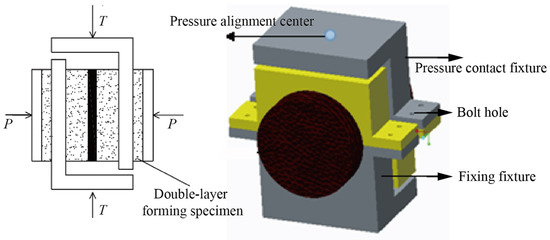
Figure 5. Diagram of the horizontal shear fixture.

4. Experimental Investigations

4.1. Specimen Design

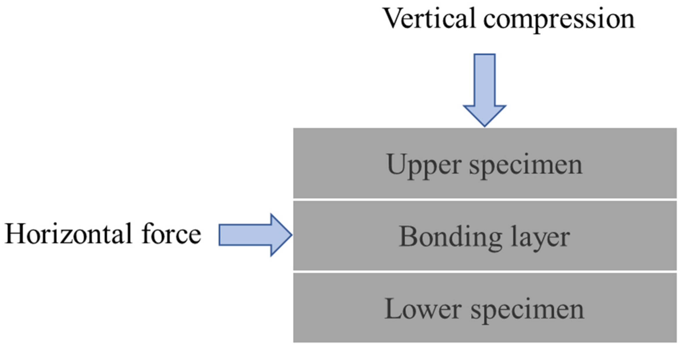
In order to simulate the working state of the middle layer in the actual engineering, the specimen adopts the structure “upper specimen + bonding layer + lower specimen”, as shown in Figure 6.

Figure 6. Schematic diagram of the specimen (actual thickness of bond layer is very thin, which can be considered as no thickness).

The two-layer specimen of asphalt mixture used in the test was obtained by SGC integral molding. The specific steps follow: (1) The specimen was formed with a lower layer of 50 mm, and cooled for 24 h; then, the surface of the specimen was spread with different specifications of adhesive oils, as shown in Figure 7a. (2) The processed specimen was placed into the SGC test mold as the base. (3) Another specimen with an upper layer of 50 mm was formed based on the previous specimen, as shown in Figure 7b. (4) The prepared SGC specimen was drilled with a diameter of 100 mm core sample, as shown in Figure 7c. The extracted core sample should be as smooth as possible, as shown in Figure 7d.

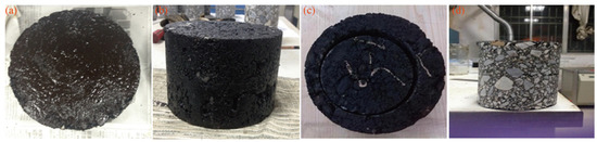
Figure 7. Images of the specimen: (a) specimen coated with adhesive oil; (b) composite specimen; (c) specimen core; (d) core sample.

The asphalt mixture and cement-stabilized mixture samples were obtained by in situ drilling for core sampling and SGC molding. The specific steps are as follows: (1) A road surface detection coring machine with a diameter of 150 mm is used to core the cement-stabilized base after 28 days of health maintenance, and the height of each core sample was recorded with a vernier caliper. (2) The cement stable-base core sample was placed into the test mold, and then the upper asphalt mixture was poured into the test mold quickly, and the top surface covered with a filter paper. (3) The molding height of the compacting instrument was set as core sample height (50 mm), and then the steps of forming the asphalt mixture double-layer specimen and core sample drilling were repeated.

4.2. Test Steps

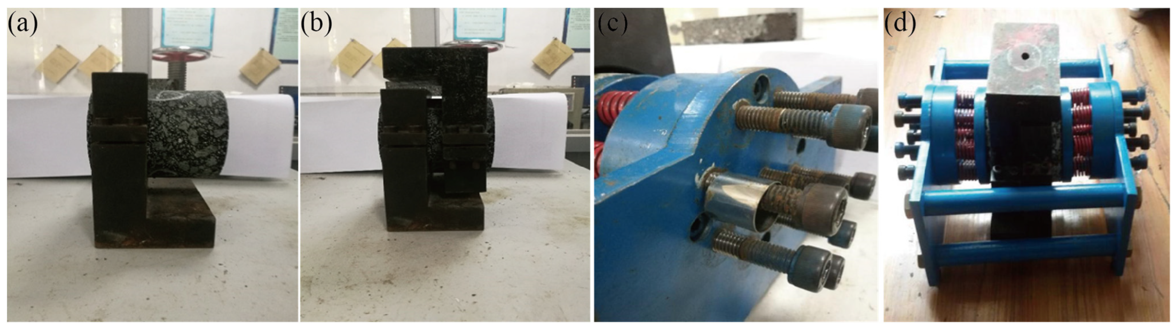
The installation steps of the specimen follow: (1) The specimen was installed on the fixture, the interlayer interface was kept 5 mm from the right end of the fixture, and the bolts were tightened to fix the specimen, as shown in Figure 8a. (2) The clamping device was fastened with the head and the interface between layers at the left end of the clamping device, and kept about 5 mm apart. The bolts were tightened to fix the specimen, as shown in Figure 8b. (3) The frame splint part and the springs on both sides of which the vertical force is applied were taken out, and calibrated with a press. (4) The frame was placed at both ends of the specimen, and the screws were inserted with a stainless steel sleeve to fix the amount of spring compression. The screws were turned with an inner hexagon wrench until they just contacted the sleeve, as shown in Figure 8c. (5) The whole specimen was placed on the UTM, and the pressure bar was aligned with the center of the pressure-head contact fixture, as shown in Figure 8d.

Figure 8. The process of test device installation: (a) mounting fixture; (b) installing the head contact clamp; (c) prefabricated stainless steel sleeve controls the spring compression; (d) image showing the completed fixture installation.

5. Analysis of Test Results

According to the experimental scheme, four kinds of experimental temperatures, four kinds of oil distributions, and two kinds of vertical pressures were selected as variables to study. AC-13 and AC-20 were the interlayer interfaces most sensitive to the wheel load. Therefore, these interlayer interfaces were selected as the research object, and the vertical compressive stress was set at 0.7 MPa. The specific experimental parameters are shown in Table 8.

Table 8. Experimental parameters of interlayer interface model.

Experimental Variable	Experiment with the Selected Variables
Upper layer	AC-13
Following layer	AC-20
Viscosity-level	Viscosity-level oil A and B
Experimental temperature	−10, 0, 25, 50 °C
Amount of viscosity-level oil spread	0, 0.5, 1.0, 1.5 kg/m2
Vertical compression stress	0.7 MPa

By controlling these variables, interlayer direct shear tests were carried out on the double-layer specimens that were formed, and the effects of different temperatures and vertical compressive stress on the bonding coefficient were compared under the same spreading amount of oil in the viscosity-level.

5.1. Influence of Temperature

Temperature has a strong influence on the adhesion oil of emulsified asphalt, and then affects the interlayer characteristics. In this section, adhesion coefficient $K_{\max }$ is selected as an evaluation index of interlayer bonding capacity. Experimental data are shown in Figure 9 and Figure 10.

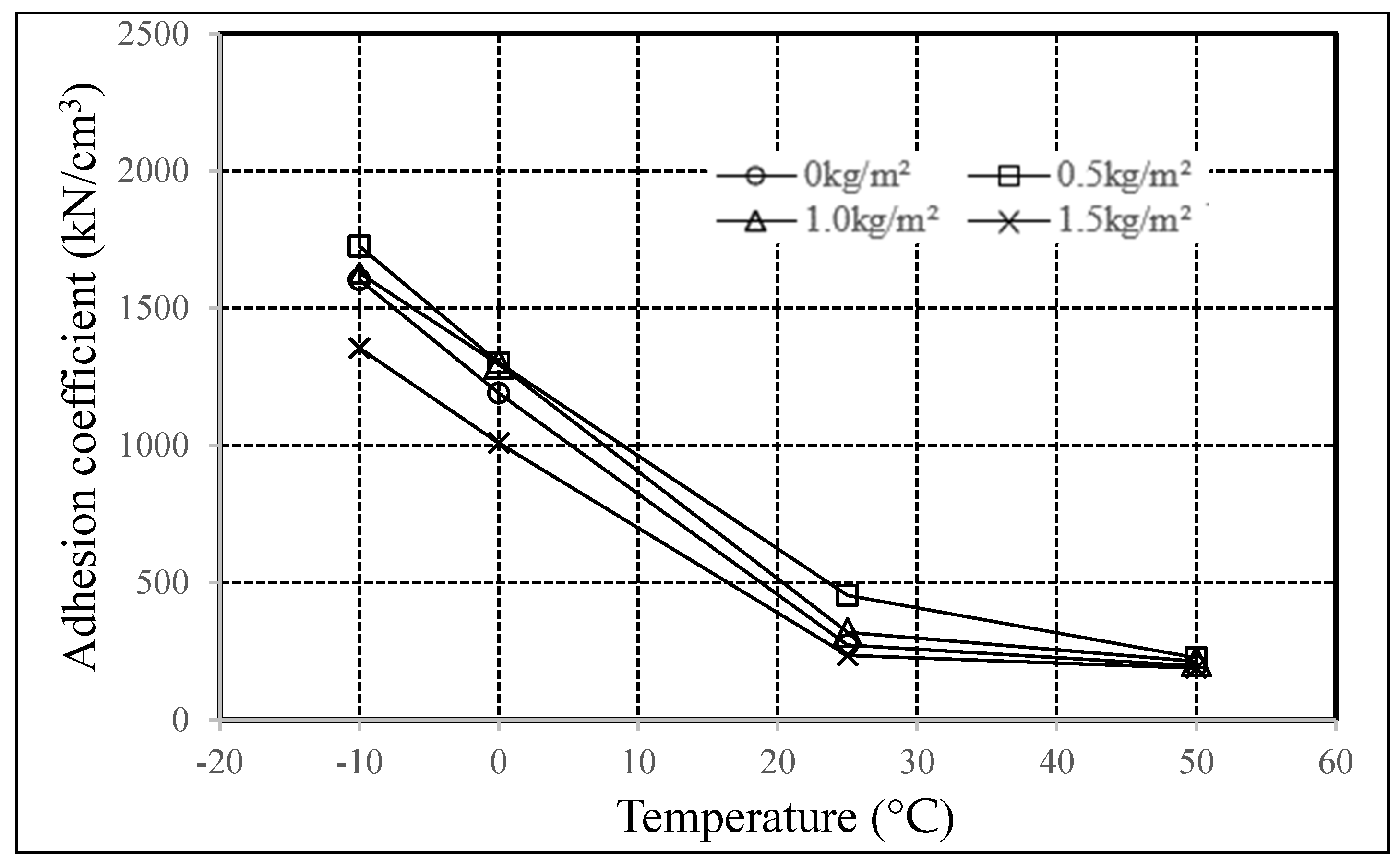
Figure 9. Influence of temperature on the bonding coefficient of oil A bond specimen.

Figure 10. Influence of temperature on the bonding coefficient of oil B bond specimen.

It can be seen from Figure 9 and Figure 10 that the value of adhesion coefficient K gradually decreases with the increase in temperature, indicating that the higher the temperature, the weaker the interlayer bonding ability and the more vulnerable it is to damage.

We know that there are three stages in the variation of the adhesion coefficient with the change in temperature. When the temperature rises from −10 to 0 °C, the average adhesion coefficients of oil A and oil B bond specimens decrease by 27.3% and 23.5%, respectively. When the temperature rises from 0 to 25 °C, the average adhesion coefficients of oil A and oil B bond specimens decrease by 65.7% and 72.0%, respectively. However, when the temperature rises from 25 to 50 °C, the average adhesion coefficients of oil A and oil B bond specimens are almost the same. It can be seen that the type of the viscosity-level oil has a significant influence on interlayer bonding performance at room temperature and below. When the temperature is high, this difference is small.

5.2. Influence of the Spreading Amount of Viscosity-Level Oil

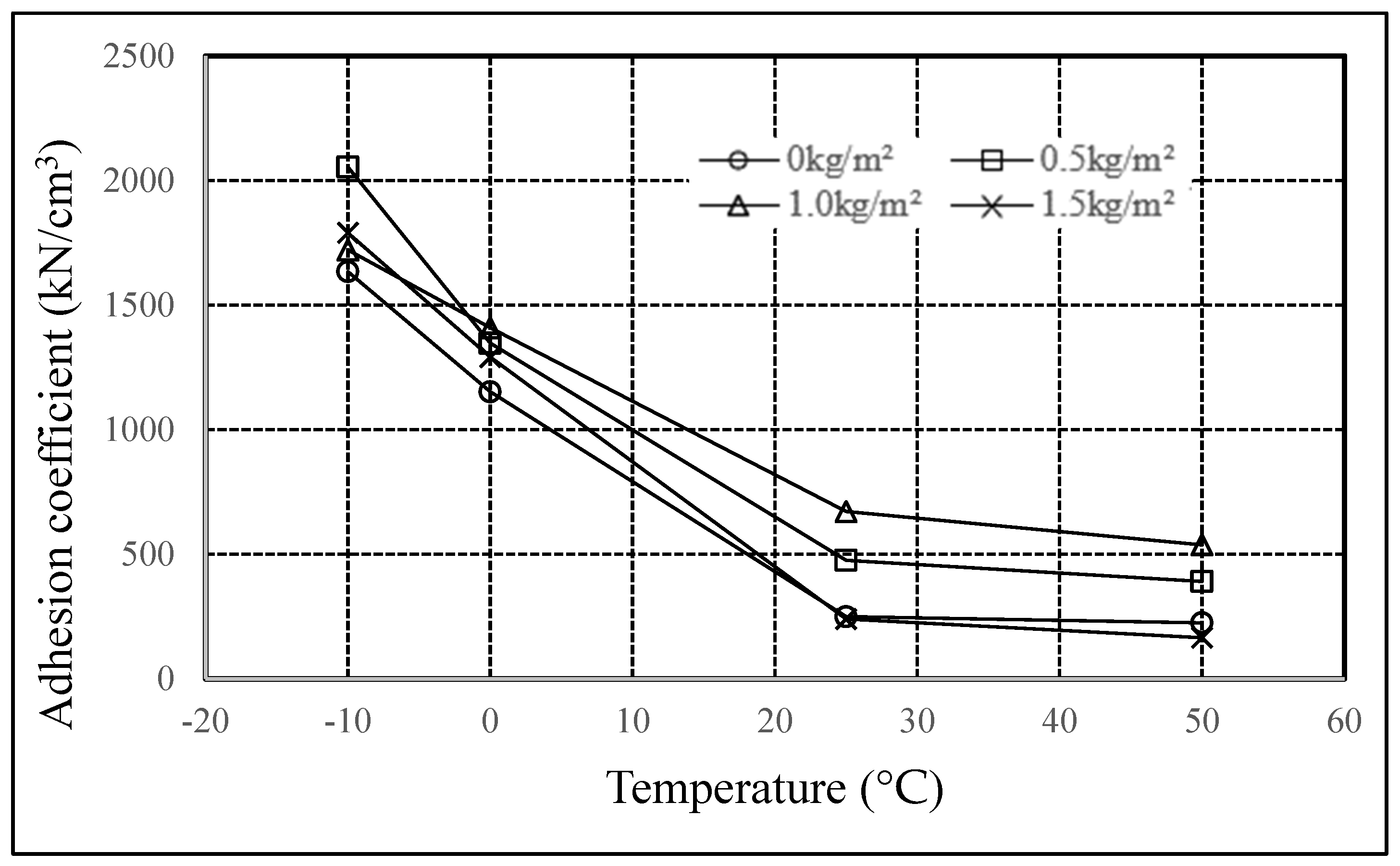
In order to further study the influence of different spreading amount of the viscosity-level oil on interlayer interface characteristics under vertical load, the maximum adhesion coefficient K_max was selected as the evaluation index of interlayer adhesion capacity, and relevant tests are carried out. The experimental data are shown in Figure 11 and Figure 12.

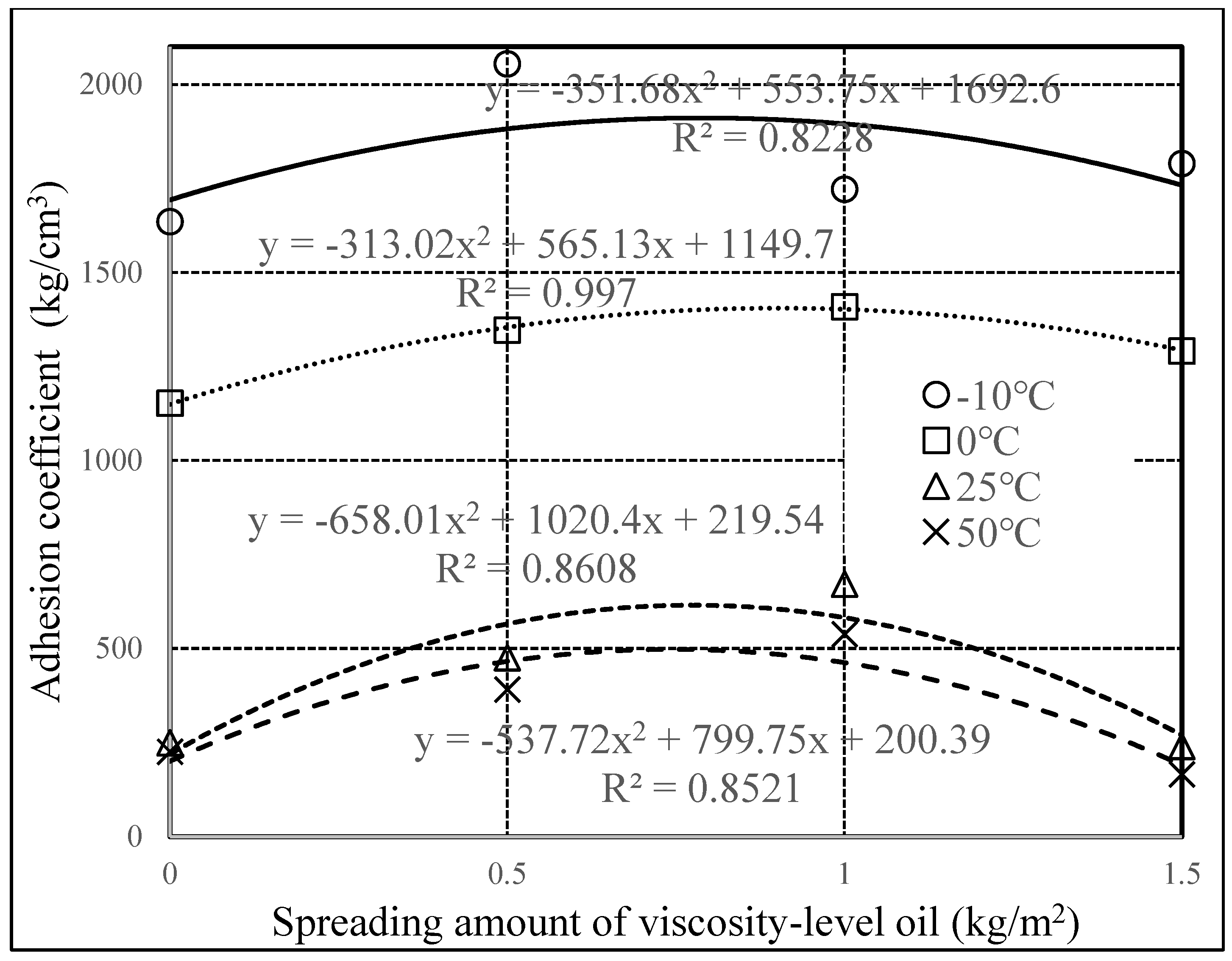
Figure 11. The curves relating spreading amount of viscosity-level oil A and adhesion coefficient.

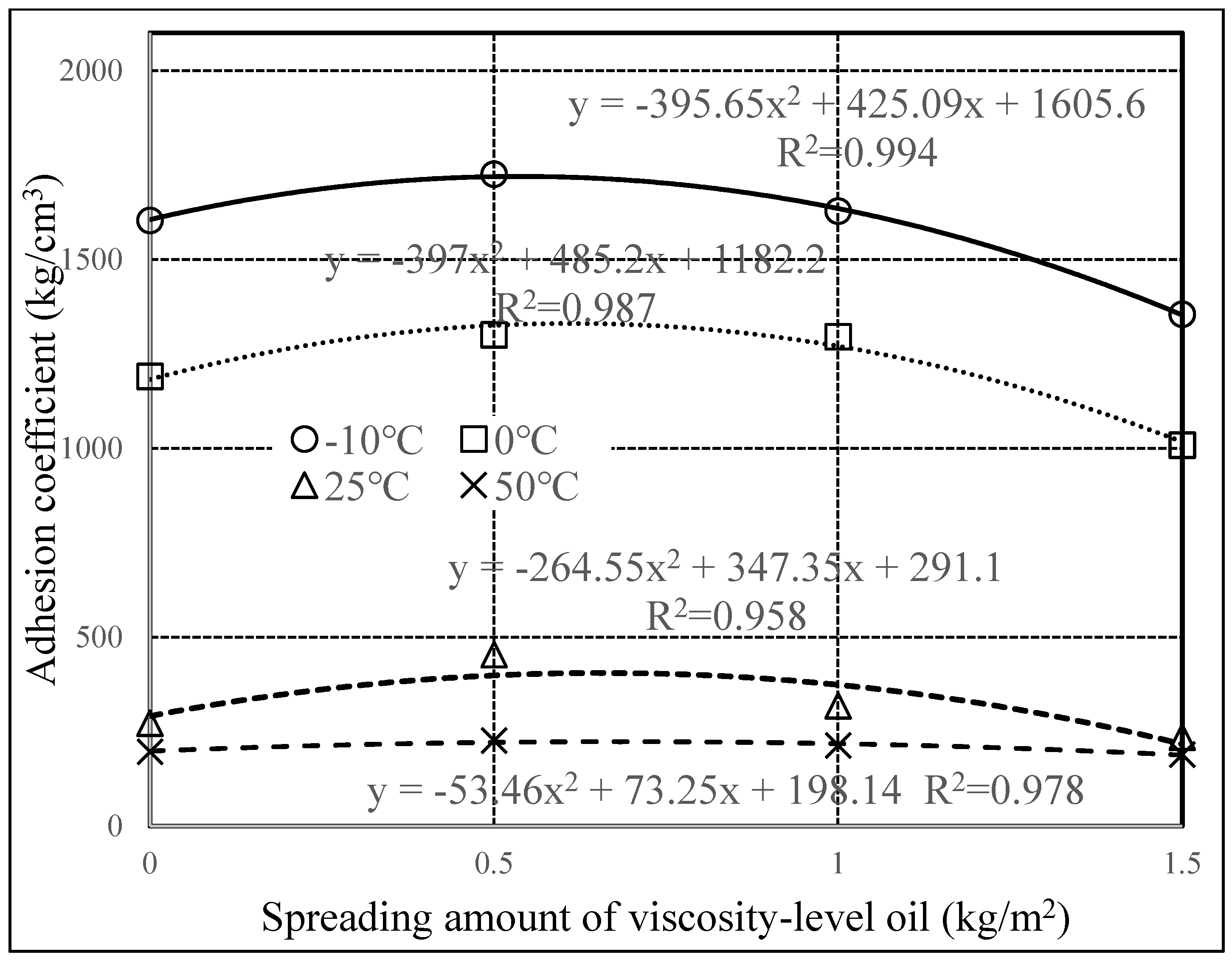
Figure 12. The curves relating spreading amount of viscosity-level oil B and adhesion coefficient.

Figure 11 and Figure 12 show the following features:

(1)

When the ambient temperature is −10 °C, the change in adhesion coefficient of viscosity-level oil A is not obvious. When the spreading amount increases from 0 to 0.5 kg/m², the adhesion coefficient increases by 25.7%. However, when the spreading amount changes from 0.5 to 1.5 kg/m², the change in the adhesion coefficient is small. In contrast, the adhesion coefficient of viscosity-level oil B is more regular, and the adhesion coefficient increases first and then decreases, with an obvious peak value.

(2)

When the ambient temperature is 0 °C, the adhesion coefficient of viscosity-level oil A shows an obvious regularity. The adhesion coefficient increases first and then decreases with the spreading amount increasing from 0 to 1.5 kg/m². Similarly, the regularity of the adhesion coefficient for viscosity-level oil B is consistent with viscosity-level A.

(3)

When the ambient temperature is 25 °C, the adhesion coefficient increases by 90.9% with the spreading amount of viscosity-level oil A increasing from 0 to 0.5 kg/m². When the spreading amount ranges from 0.5 to 1.0 kg/m², the adhesion coefficient increases by 41.3%. When the spreading amount increases from 1.0 to 1.5 kg/m², the adhesion coefficient decreases sharply by 64.4%. However, when the spreading amount of viscosity-level oil B increases from 0 to 0.5 kg/m², the adhesion coefficient increases by 66.5%. When the spreading amount increases from 0.5 to 1.0 kg/m², the adhesion coefficient decreases by 29.8%. When the spreading amount increases from 1.0 to 1.5 kg/m², the adhesion coefficient decreases by 26.1%.

(4)

When the ambient temperature is 50 °C, the adhesion coefficient of viscosity-level oil A is consistent with that at 25 °C. When the spreading amount increases from 0.5 to 1.0 kg/m², the adhesion coefficient increases by 37.7%. When the spreading amount increases from 1.0 to 1.5 kg/m², the adhesion coefficient decreases sharply by 69.3%. The change in adhesion coefficient of viscosity-level oil B is not obvious, but it still shows a trend of first increasing and then decreasing.

In general, the spreading amount of viscosity-level oil has a certain effect on the adhesion coefficient. From 0 to 1.5 kg/m², the adhesion coefficient increases gradually first and then decreases, which basically shows a downward parabola form. Therefore, there is an optimal spreading amount. By fitting the curves of Figure 11 and Figure 12, the polynomials are shown in Table 9, and the optimal amount of viscosity oil can be obtained under different working conditions.

Table 9. The best range of adhesive oil spread.

Temperature	Viscosity-Level Oil A	Kmax Corresponds to the Spreading Amount of Viscosity-Level Oil	Viscosity-Level Oil B	Kmax Corresponds to the Spreading Amount of Viscosity-Level Oil
−10 °C	y = −351.68x2 + 553.75x + 1692.6	0.78 kg/m2	y = −395.65x2 + 425.09x + 1605.6	0.54 kg/m2
0 °C	y = −313.02x2 + 565.13x + 1149.7	0.90 kg/m2	y = −397x2 + 485.2x + 1182.2	0.61 kg/m2
25 °C	y = −658.01x2 + 1020.4x + 219.54	0.78 kg/m2	y = −264.55x2 + 347.35x + 291.1	0.65 kg/m2
50 °C	y = −537.72x2 + 799.75x + 200.39	0.74 kg/m2	y = −53.46x2 + 73.25x + 198.14	0.68 kg/m2

It can be seen from Table 9 that the spreading amounts of the viscosity-level oil A and oil B corresponding to their maximum adhesion coefficients, which are about 0.8 and 0.6 kg/m², respectively, at different temperatures. Therefore, the optimal spreading amount of the viscosity-level oil is suggested to be 0.6~0.8 kg/m².

5.3. Influence of Type of Viscosity Oil

The viscosity-level oil A and B are quick-cracking emulsified asphalt. The main difference is that the content of evaporative residue of oil A is 59.4% and that of oil B is 64.1%. The penetration and elongation of the evaporative residue in oil A are 140% and 53% higher than that in oil B. Specific experimental data are shown in Figure 13, Figure 14, Figure 15 and Figure 16.

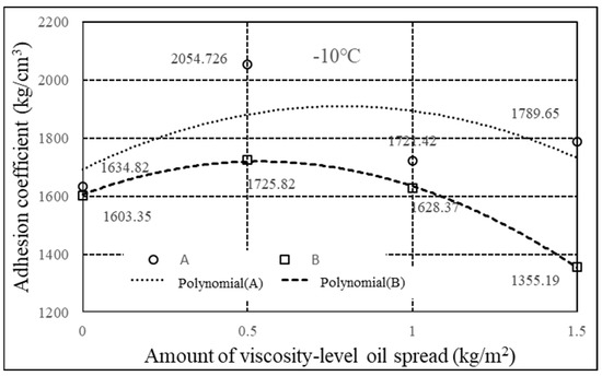
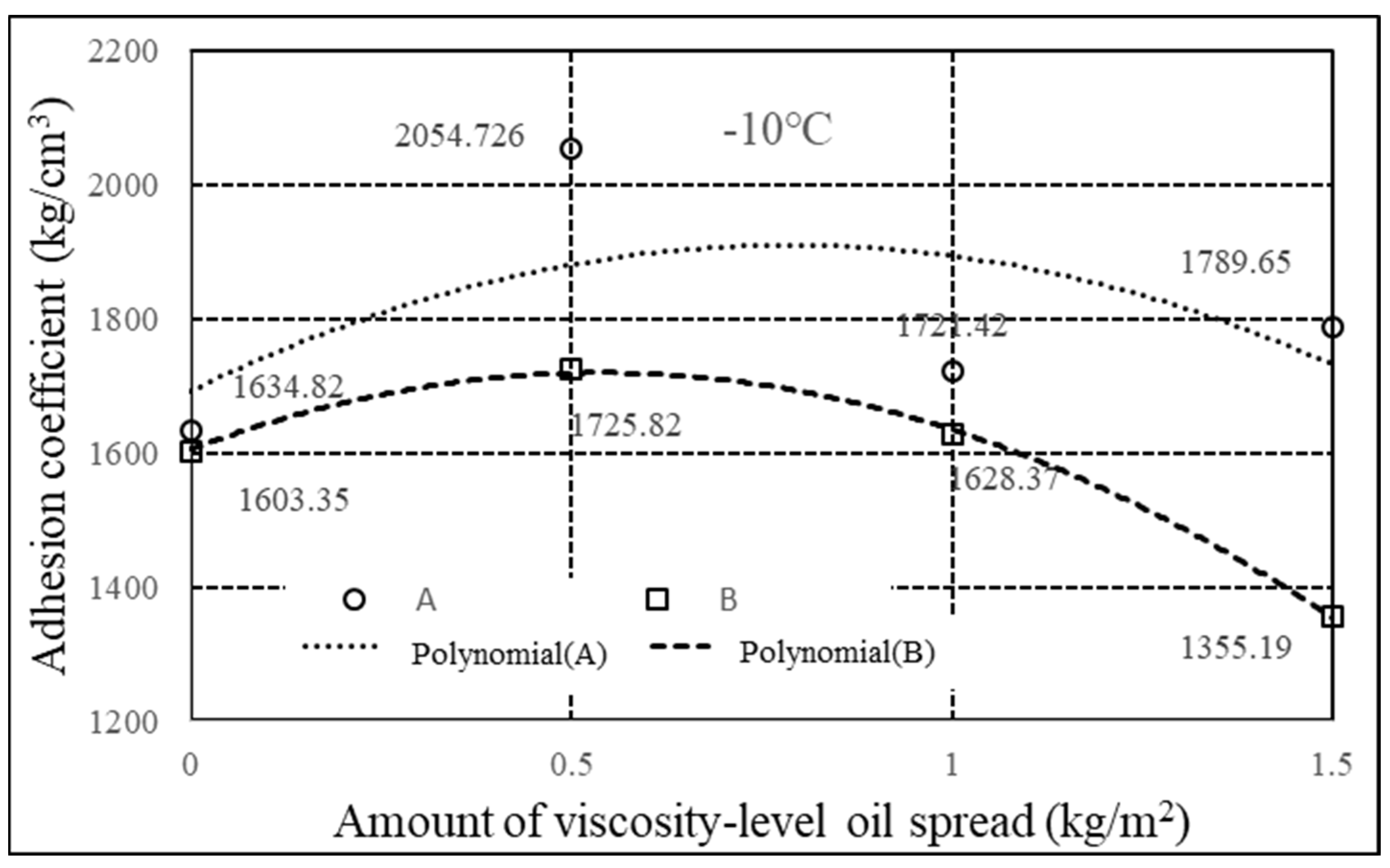
Figure 13. Adhesion coefficient curve of viscosity-level oil A and B specimens at −10 °C.

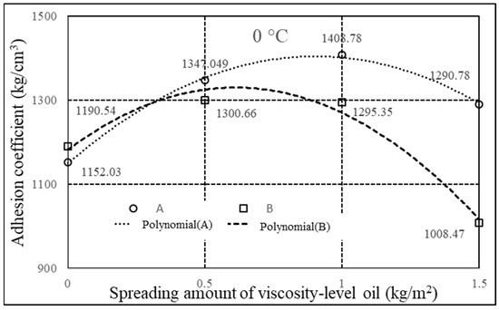
Figure 14. Adhesion coefficient curve of viscosity-level oil A and B specimens at 0 °C.

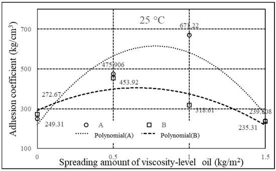
Figure 15. Adhesion coefficient curve of viscosity-level oil A and B specimens at 25 °C.

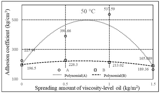
Figure 16. Adhesion coefficient curve of viscosity-level oil A and B specimens at 50 °C.

At the different temperatures, viscosity-level A and B have corresponding adhesion coefficients under different spreading amounts, and the polynomial curve is fitted according to the measured values. Figure 13, Figure 14, Figure 15 and Figure 16 show the following features:

(1)

When the ambient temperature is −10 °C, the adhesion coefficient corresponding to the three spreading amounts of viscosity-level oil A is superior to that for viscosity-level oil B. However, the spreading amounts of viscosity-level oil A are 1.0 and 1.5 kg/m², and their maximum adhesion coefficients $K_{\max }$ are close. Therefore, the trend line of viscosity-level oil A does not have obvious regularity.

(2)

The maximum adhesion coefficients $K_{\max }$ of viscosity-level oil A and B are almost the same when the spreading amount is 0.5 kg/m² and the ambient temperature is 0 °C. With the increase in the spreading amount, the $K_{\max }$ increases first and then decreases, while that of oil B decreases, obviously.

(3)

When the ambient temperature is 25 °C, the $K_{\max }$ of viscosity-level oil A is obviously better than that for oil B only when the spreading amount is 1.0 kg/m².

(4)

The maximum adhesion coefficient $K_{\max }$ of viscosity-level oil A has an obvious trend, while the $K_{\max }$ of oil B remains essentially unchanged at the 50 °C ambient temperature.

According to the above analysis, it can be found that $K_{\max }$ has changes significantly when the ambient temperature is low; however, the trend is not obvious at high ambient temperature. The main reason is that asphalt is a temperature-sensitive material, and the temperature change has a strong impact on it. At high temperature, the softening viscosity drops sharply, which causes the interlayer shear resistance to decrease, and then the interlayer interlocking effect decreases and the bonding state weakens sharply. Note that the difference in effect caused by different types of viscosity-level oil has not been analyzed. Experimental results indicate that it is mainly related to the performance index of its evaporation residue. Overall, the interlayer bonding effect of viscosity-level oil A is superior to that of oil B.

5.4. Influence of Vertical Load and Interlayer Characteristics between the Asphalt Layer and Base Layer

In the preceding sections, the vertical load is applied at 0.7 MPa, which simulates the stress situation between the upper layer and the middle layer of asphalt. Owing to the diffusion of force, the vertical load between the asphalt surface layer and the lower layer, the lower layer and the base, is not 0.7 MPa, but reduced by a certain degree. Therefore, the vertical compressive stress of three asphalt layers is calculated by means of mechanical calculation, and this is used as the basis for the vertical load in the laboratory. Based on the results of experiment and calculation, the best value for the spreading amount is recommended. The vertical compressive stress between AC-20 and AC-25 is calculated by ANSYS software to be 0.16 MPa, and the vertical compressive stress between AC-25 and the cement-stabilized base layer is 0.07 MPa. Specific experimental parameters are shown in Table 10. According to the above description, it can be found that the interlayer bonding behavior of oil A is superior to that of oil B under comprehensive conditions.

Table 10. Experimental parameters to verify the effect of vertical load.

Experimental Variable	Experiment with the Selected Variables
Upper layer	AC-20, AC-25
Following layer	AC-25, Cement-stabilized crushed stone
Viscosity-level	Viscosity-level oil A, Site sampling of transparent layer of oil A
Experimental temperature	−10, 0, 25, 50 °C
Amount of viscosity-level oil spread	0, 0.5, 1.0, 1.5 kg/m2
Vertical compression stress	0.16, 0.07 MPa

The corresponding interlayer shear test was carried out as described in the previous section. The adhesion coefficient $K_{\max }$ between the AC-20 and AC-25 layers is shown in Figure 17.

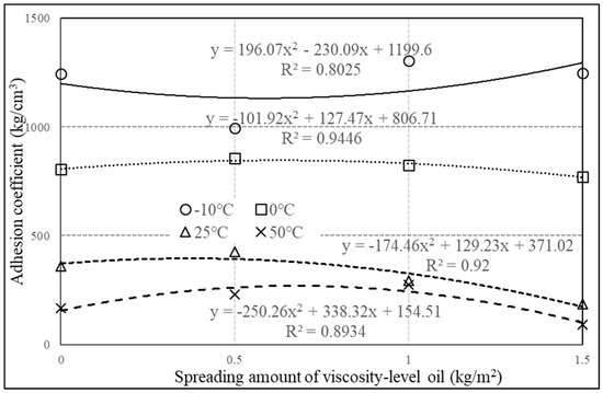
Figure 17. The $K_{\max }$ curves of AC-20/AC-25.

As can be seen from Figure 17, the maximum adhesion coefficient between layers is not regular when the temperature is −10 °C, and the adhesion coefficient is not only affected by the structural depth on the surface of the two specimens, but also has a strong relationship with the adhesion between the asphalt film and the cohesion of the viscosity-level oil. Therefore, the influence of the amount of viscosity oil on the interlayer interface is not obvious under such low temperature conditions. When the ambient temperature is 0, 25, and 50 °C, then $K_{\max }$ increases first and then decreases in the upper and middle layers.

In general, the spreading amount of viscosity oil has a certain effect on the adhesion coefficient between layers in asphalt. From 0 to 1.5 kg/m², $K_{\max }$ gradually increases first and then decreases, basically presenting a parabolic form with downward opening. Therefore, there is an optimal spreading amount. By fitting the curve of Figure 17, the polynomial is obtained, as shown in Table 11; thus, the optimal spreading amount of viscosity oil can be obtained under different working conditions.

Table 11. Optimum amount of viscosity oil spread.

Temperature	Viscosity Oil A	Kmax Corresponds to the Spreading Amount of Viscosity-Level Oil
−10 °C	y = 196.07x2 − 230.09x + 1199.6	/
0 °C	y = −101.92x2 + 127.47x + 806.71	0.63 kg/m2
25 °C	y = −174.46x2 + 129.23x + 371.02	0.37 kg/m2
50 °C	y = −250.26x2 + 338.32x + 154.51	0.67 kg/m2

It can be seen from Table 11 that the interlayer adhesion coefficient reaches its maximum value when the spreading amount is controlled in the range 0.4~0.7 kg/m² at the ambient temperature 0~50 °C.

The characteristics of the interlayer adhesion coefficient between AC-25 and the cement-stabilized macadam base are also tested and analyzed, and the test results are shown in Figure 18.

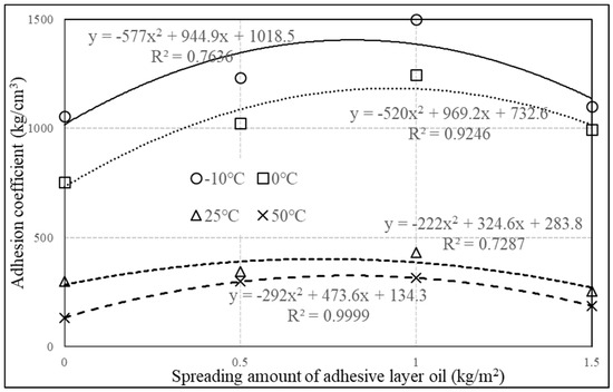
Figure 18. The K_max curves of AC-25/ cement-stabilized base.

Owing to the large void ratio of AC-25 and cement-stabilized macadam base mixture, a large amount of viscosity-level oil is absorbed into the specimen. At low temperature, the interlayer adhesion coefficient $K_{\max }$ increases obviously when the amount of spread increases from 0 to 1.0 kg/m². However, $K_{\max }$ decreases about 25% when the amount of spread increases to 1.5 kg/m².

By fitting the curves of Figure 18, the polynomial can be obtained, as shown in Table 12, and the optimal spreading amount of the transparent layer of oil under different working conditions can be determined.

Table 12. Optimum spreading amount of transparent layer of oil.

Temperature	Transparent Layer of Oil A	Kmax Corresponds to the Spreading Amount of Viscosity-Level Oil
−10 °C	y = −577x2 + 944.9x + 1018.5	0.82 kg/m2
0 °C	y = −520x2 + 969.2x + 732.6	0.93 kg/m2
25 °C	y = −222x2 + 324.6x + 283.8	0.73 kg/m2
50 °C	y = −292x2 + 473.6x + 134.3	0.81 kg/m2

It can be concluded from Table 12 that the interlayer adhesion capacity between the asphalt layer and the water-stable base reaches a maximum when the amount of transparent layer of oil is controlled at 0.7~1.0 kg/m².

6. Conclusions

This paper investigates the characteristics of interlayer interface of asphalt pavement under vehicle load by using a self-modified test fixture. The related parameters, including room temperatures, gradation, amount of spread, viscosity-level oil types, and vertical compressive stress, are considered and the change rule of interlayer interface between asphalt pavement under vertical load based on Goodman model is analyzed. Some broad conclusions are summarized:

(1)

Temperature has a strong influence on the viscosity-level oil of emulsified asphalt, and then affects the interlayer characteristics. When the temperature rises from −10 to 25 °C, the average adhesion coefficient of the specimen decreases by 70~80%. However, when the temperature is above 25 °C, the influence of temperature on the adhesion coefficient gradually decreases.

(2)

In the case of constant vertical load, the spreading amount of viscosity-level oil also has a strong influence on the adhesion state of the interlayer interface. The adhesion coefficient increases first and then decreases with the spreading amount increasing from 0 to 1.5 kg/m². The best adhesion coefficient is obtained for the spreading amount range 0.5~1.5 kg/m².

(3)

By comparing the adhesion properties of viscosity-level oil A and B at different temperatures, it is found that the adhesion properties of viscosity-level oil A are superior to oil B.

(4)

The optimal spreading amounts of viscosity-level oil between layers in the asphalt concrete pavement structure are recommended: 0.6~0.8 kg/m² between AC-13 and AC-20 asphalt structural layers; 0.4~0.7 kg/m² between AC-20 and AC-25 asphalt structural layers, and 0.7~1.0 kg/m² between AC-25 and water stabilized base.

References

- Ning, Z.F. Analysis and Evaluation of Interlayer Combination of Asphalt Pavement; Hunan University: Changsha, China, 2012. [Google Scholar]
- Fang, H.; Luo, H.; Zhu, H. The feasibility of continuous construction of the base and asphalt layers of asphalt pavement to solve the problem of reflective cracks. Constr. Build. Mater. 2016, 119, 80–88. [Google Scholar] [CrossRef]
- JTG D50-2017; Specifications for Design of Highway Asphalt Pavement. People’s Communications Publishing House: Beijing, China, 2017.
- JTG F40-2004; Technical Specification for Construction of Highway Asphalt Pavement. People’s Communications Publishing House: Beijing, China, 2004.
- Liu, H.M.; Song, X.D.; Huo, Y.G.; Zhou, Y. Development and application of shear stress measuring instrument between layers of asphalt pavement. J. Xian Univ. Sci. Technol. 2014, 34, 119–122. [Google Scholar]
- Cho, S.H. Evaluation of Interfacial Stress Distribution and Bond Strength between Asphalt Pavement Layers; North Carolina State University: Raleigh, NC, USA, 2015. [Google Scholar]
- Livneh, M.; Shklarsky, E. The bearing capacity of asphalt concrete surfacing. In Proceedings of the 1st: International Conference on the Structural Design of Asphalt Pavements; University of Michigan: Ann Arbor, MI, USA, 1962; pp. 345–353. [Google Scholar]
- Goodman, R.E.; Brekke, T.L. A model for the mechanics of jointed rock. J. Mech. Found. Div. 1968, 94, 637–659. [Google Scholar] [CrossRef]
- Uzan, J.; Livneh, M.; Eshed, Y. Investigation of adhesion properties between asphalt concrete layers. Asph. Paving Technol. 1978, 4, 495–521. [Google Scholar]
- Romanoschi, S.A.; Metcalf, J.B. The characterization of asphalt concrete layer interfaces. In Proceedings of the Ninth International Conference on Asphalt Pavements, Copenhagen, Denmark, 17–22 August 2002. [Google Scholar]
- Mariana, R.; Kruntchev, A.; Andrew, C. Effect of Bond Condition on Flexible Pavement Performance. J. Transp. Eng. 2005, 130, 880–888. [Google Scholar]
- Leng, Z.; Ozer, H.; Al-Qadi, H.I.; Carpenter, H.S. Interface bonding between hot-mix asphalt and various Portland cement concrete surfaces. Transp. Res. Rec. 2008, 2057, 46–53. [Google Scholar] [CrossRef]
- Kruntcheva, M.R.; Collop, A.C.; Thom, N.H. Properties of Asphalt Concrete Layer Interfaces. Am. Soc. Civ. Eng. 2013, 18, 467–471. [Google Scholar] [CrossRef]
- Hu, X.D.; Walubita Lubinda, F. Effects of Layer Interfacial Bonding Conditions on the Mechanistic Responses in Asphalt Pavements. J. Transp. Eng. 2010, 137, 28–36. [Google Scholar] [CrossRef]
- Wang, S.Y. Study on Test Method of Interlayer Shear Strength of Indoor Asphalt Concrete Pavement. Highway 2010, 2, 144–147. [Google Scholar]
- Liu, F.Q. Influence of Interlaminar Shear Stress among Layers of Asphalt Pavement with Semi-rigid Base on Its Distortion Energy. J. Lanzhou Inst. Technol. 2016, 23, 10–13. [Google Scholar]
Publisher’s Note: MDPI stays neutral with regard to jurisdictional claims in published maps and institutional affiliations. |
© 2022 by the authors. Licensee MDPI, Basel, Switzerland. This article is an open access article distributed under the terms and conditions of the Creative Commons Attribution (CC BY) license (https://creativecommons.org/licenses/by/4.0/).