Abstract
In bit-patterned media recording (BPMR) systems, the readback signal is affected by neighboring islands that are characterized by intersymbol interference (ISI) and intertrack interference (ITI). Since increasing the areal density encourages the influence of ISI and ITI, it is more difficult to detect the data. Modulation coding can prevent the occurrence of specific data patterns that can cause severe ISI and ITI. In this study, we propose a modulation decoding method based on the K-means algorithm for a BPMR system to improve decoding capabilities. As the K-means algorithm helps understand data patterns and characteristics, the K-means decoder shows the best performance.
1. Introduction
The rapid growth of the Internet and communication systems has generated an enormous amount of data. Data storage systems have therefore been growing rapidly to accommodate increasing capacity. However, the magnetic storage industry faces the problem of superparamagnetic effects, which restricts increase in areal density to around one terabit per square inch (Tb/in2) [1]. To overcome this problem and increase the areal density of magnetic materials, bit-patterned media recording (BPMR) systems are considered as promising technologies for next-generation magnetic storage [2]. In BPMR, a nanoscale magnetic island can store one bit, and each island is surrounded by a nonmagnetic material. The use of the BPMR system can reduce transition noise, track edge noise and nonlinear bit shift, and simplify tracking [3]. However, conventional magnetic storage systems suffer from one-dimensional (1D) interference, and using BPMR poses a new risk called two-dimensional (2D) interference that consists of intersymbol interference (ISI) and intertrack interference (ITI) [4]. As the readback signal in recording systems is subject to 2D interference and noise that limits the reliability of the system, ISI and ITI are major obstacles that degrade system performance. Moreover, 2D interference can become more severe because the spacing between islands is reduced to achieve a higher areal density.
Unlike typical communication systems with retransmission processing, data storage systems have difficulty in retransmitting data. In addition, a low probability of decoding failure is strictly required for data storage systems, and the goal in data storage systems is to achieve bit error rate (BER) of 10−12 or better [5]. In data storage systems, signal detection, error-correcting coding (ECC), and modulation coding are employed to recover data corrupted by interference and noise. Signal detection is applied to data storage systems to combat interference, and a partial-response maximum-likelihood (PRML) detector is used to perform signal detection in data storage systems [6,7]. ECC techniques transform data sequences into better sequences by using redundant bits for the detection and correction of errors. Low-density parity check codes providing near-capacity performance on storage channels are currently used in data storage systems [5,8]. Modulation coding helps increase the detection capabilities of a data storage system by imposing constraints [9,10]. As data storage systems are susceptible to errors in specific data patterns, modulation coding is used to restrict troublesome patterns.
Recently, several signal processing schemes with machine learning for communication and data storage system channels have been studied to improve decoding capabilities and system performance. In [11], the equalizer technique based on a multilayer perceptron (MLP) was discussed. The MLP equalizer outperforms the conventional equalizer because the MLP equalizer can solve the linear and nonlinear phenomena of the channels. In [12], the neural-network-based modulation decoding of constrained sequence codes like run-length-limited code and DC-free code was introduced and evaluated in wireless channels. The iterative detection technique with MLP was proposed to decrease the effect of ITI and improve the performance [13]. In [14], a bit-flipping scheme using the K-means algorithm was proposed to flip a sign of data that is predicted to be an error. However, these works using machine learning algorithms were applied to signal detection without modulation decoding.
Modulation codes are generally used to mitigate ISI which occurs in the data storage systems by imposing constraints. To improve the capability of the modulation decoder, the machine learning algorithm was applied as the decoding algorithm. In [15], the modulation decoding technique using MLP was proposed. However, the MLP, which is a supervised learning technique, requires labeled data and a training process, making it very costly and time-consuming.
In this paper, we propose a modulation decoding method based on the K-means algorithm for a BPMR system to improve decoding capabilities. The K-means algorithm is an unsupervised learning algorithm which does not require labeled data and training processes and automatically groups data into clusters [16]. To utilize these advantages, we apply the K-means algorithm for the decoding algorithm. The proposed modulation decoding method based on the K-means algorithm can consider the geometrical distance between received codewords used depending on the characteristics or patterns of the received data sequences.
The rest of this paper is organized as follows. In Section (2), we introduce the BPMR channel model and PRML detector. Section (3) explains the proposed modulation decoding scheme using MLP, and Section (4) contains the simulation and results. Finally, Section (5) concludes the paper.
2. Channel Model and Detector
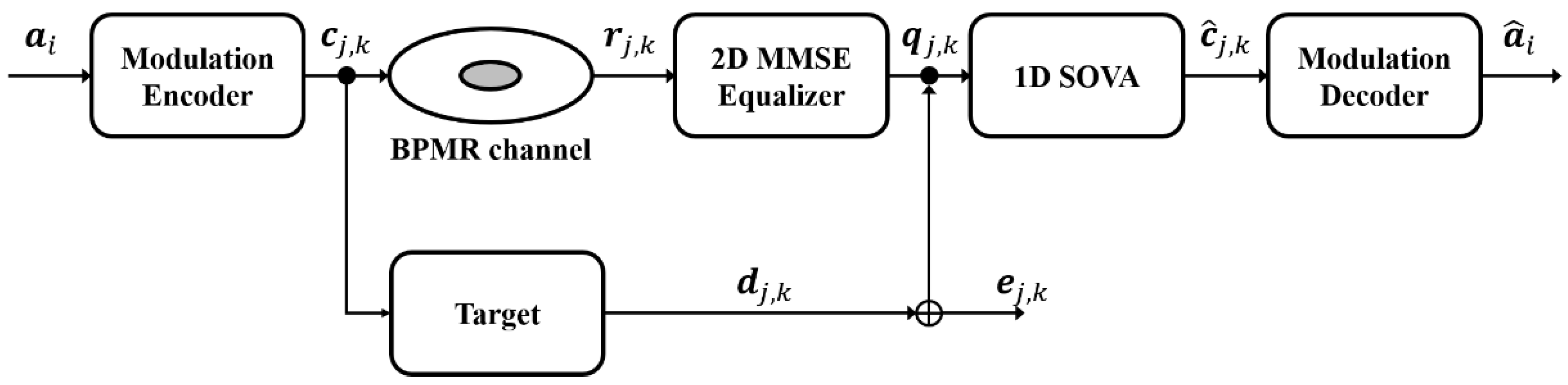
In Figure 1, we show the block diagram of a BPMR system. Before passing through the BPMR channel, the user data ak ∈ {0, 1} is encoded to the 2D array element cj,k ∈ {−1, +1} using a modulation encoder. For BPMR channel modeling, a numerical 2D Gaussian pulse response H(z, x) can be written as [17,18]:
where A = 1 is the peak amplitude of the pulse response, c = 1/2.3548 is the constant that represents the relationship between PW50 and the standard deviation of a Gaussian function, z and x are the time indices in cross- and down-track directions, respectively, PWz = 24.8 nm and PWx = 19.4 nm are the PW50 of the cross- and down-track pulses, and ∆TMR is the value of head offset or track-misregistration (TMR), which degrades the system performance due to the misalignment of the read-head from the main track. ∆TMR is defined as
where TMRz is the percentage of TMR. The 2D discrete channel obtained by sampling the 2D Gaussian pulse response is given by
where m and n are the indices of bit islands in the cross- and down-track directions, respectively, the track pitch Tz is the spacing of the islands in the cross-track direction, and the bit period Tx is the spacing of the islands in the down-track direction. The readback signal corrupted by electronic noise is given by
where M and N are the lengths of the interference from neighboring islands in the cross- and down-track directions, respectively, and nj,k is the electronic noise modeled as additive white Gaussian noise with zero mean and variance σ2. In this channel, we set M and N to 1.
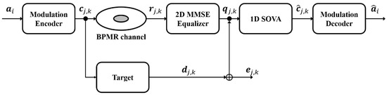
Figure 1.
Block diagram of the BPMR system model.
To address the effects of ISI and ITI, a PRML detector composed of a 2D equalizer and 1D detector was used. The 2D equalizer is determined using the minimum mean square error (MMSE) criterion [19,20]. The equalizer output qj,k and desired output dj,k are defined as
where is the equalizer coefficient, is the readback signal used as the equalizer input, is the target coefficient, and is the user data sequence. We set Mw = 1 and Nw = 5 as the equalizer, and Ng = 1 for the partial-response (PR) target. Thus, the mean square error can be expressed as
where is the auto-correlation matrix of size (2Mw + 1)(2Nw + 1) by (2Mw + 1)(2Nw + 1), is the cross-correlation matrix of size (2Mw + 1)(2Nw + 1) by (2Ng + 1), is the auto-correlation matrix of size (2Ng + 1) by (2Ng + 1), λ is the Lagrange multiplier, and J is a vector of length (2Ng + 1), such that the second element is 1 and the remaining elements are 0. By taking the derivatives of (7) with respect to λ, g, and w, we obtain the optimized target and equalizer coefficients as follows
After the readback signal rj,k is processed by the 2D MMSE equalizer, the equalizer output qj,k is decoded by the maximum-likelihood (ML) detector based on a Viterbi algorithm (VA) which outputs the hard value or a soft-output Viterbi algorithm (SOVA) which calculates the log-likelihood ratio value [21]. The equalizer output qj,k is input to the ML detector, which outputs a sequence based on the corresponding PR target. The branch metric of the detector is calculated as follows
where ti is a state; c(ti) is the decision at the state.
3. Proposed Modulation Decoding Scheme
The supervised learning that is used for classification and prediction requires a time-consuming and expensive training process and labeling data models. Additionally, models based on supervised learning should be redesigned or retrained when features of the data are changed. However, unsupervised learning exploits similarities between inputs and finds clusters of similar inputs [22]. Clustering is an unsupervised learning process in which similar data can be identified and assigned to a cluster [23,24,25]. It is widely exploited for customer segmentation, anomaly detection, and pattern recognition. Thus, we do not need to feed labeled data into models based on unsupervised learning. The K-means algorithm is capable of clustering unlabeled data in just a few iterations, which allocates n input data sequences into k categories. In this study, we use the K-means algorithm for modulation decoding to improve decoding capabilities.
3.1. Conventional Modulation Encoding and Decoding Scheme
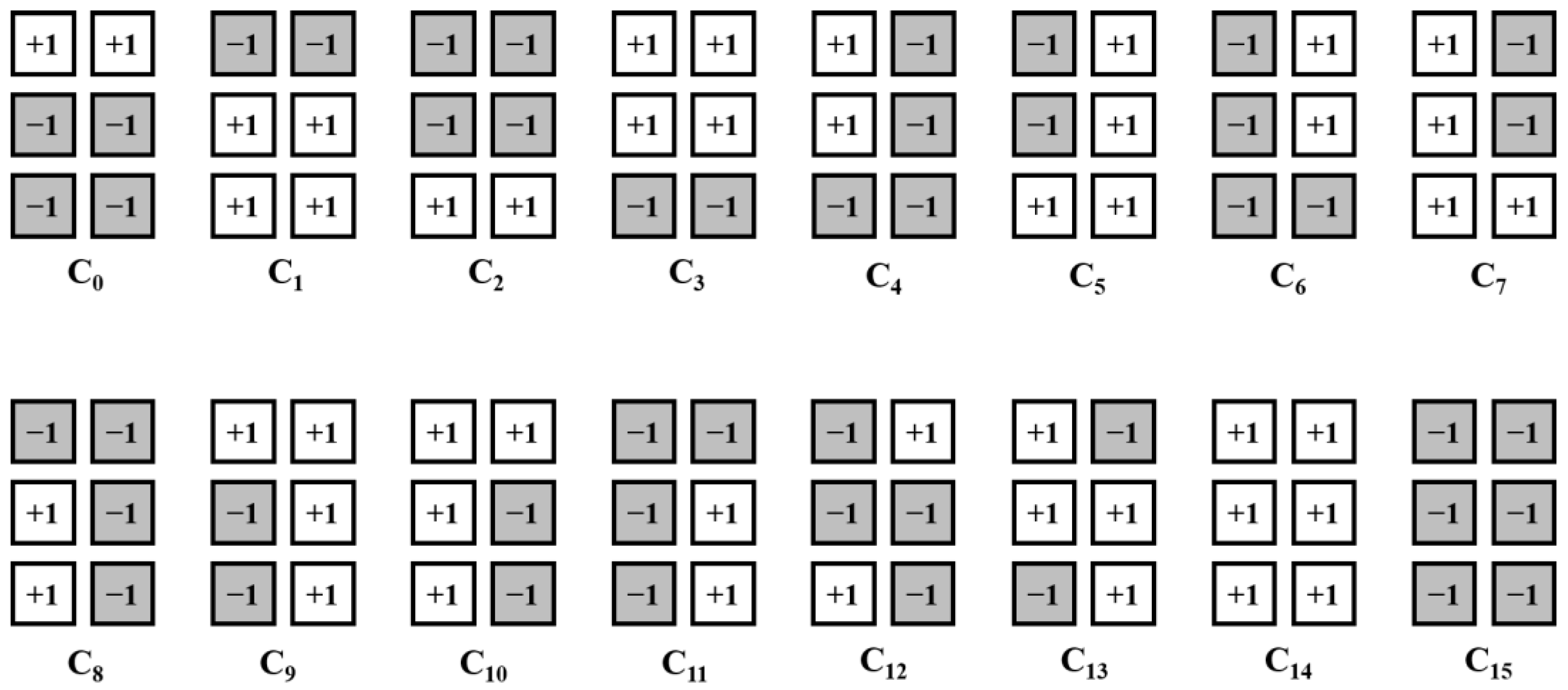
Imposing constraints in modulation coding schemes helps improve performance and eliminate patterns that cause interference. In the BPMR system, the effect of ITI has greater impact on the error performance than that of ISI, as the patterns of [−1, +1, −1]T and [+1, −1, +1]T have greater impact. To prevent patterns that degrade the performance, we used 4/6 modulation codes, and Figure 2 illustrates the codeword list of the modulation codes [15]. The codewords can prevent the occurrence of [−1, +1, −1]T and [+1, −1, +1]T in each codeword. To encode four bits a = [ai, ai+1, ai+2, ai+3] of user data to a 3 × 2 (= 6 bits) array of codewords (coded data sequences) cl = [, , , , , ] for l = 0, 1, …, 15, one-to-one mapping and a look-up table of the codeword list are used. In the decoding process, a soft decision overcomes the decoding loss of a hard decision and is mainly used to enhance the decoding process; Euclidean distance, which enables the soft decision for modulation decoding, is used. The Euclidean distance dl between the received sequence = [,, , , , ] after the VA or SOVA detector and codeword cl is calculated by

Figure 2.
Codeword list of the 4/6 modulation code.
The soft-decision decoder determines the decoded data sequence corresponding to the minimum Euclidean distance and implements one-to-one demapping.
3.2. Modulation Decoding Schemes Based on K-Means Algorithm
For modulation decoding, the received sequence must be decoded to a codeword among all codewords by the decoding algorithm. Since this process is similar to the clustering of the K-means algorithm which assigns similar instances to the corresponding clusters, we exploit the K-means algorithm for modulation decoding.
In the proposed modulation scheme, conventional modulation encoding is used in the same way, but the proposed modulation decoding is based on the K-means algorithm instead of Euclidean distance. Algorithm 1 shows the K-means algorithm. The received sequence is used as the input sequence for the algorithm. Before the algorithm is exploited, setting initialization for the number of clusters and centroids helps converge to the right solution. Since we use the 4/6 modulation code, we can set the number of clusters to 16 (the number of codewords) and centroids to [+1, +1, −1, −1, −1, −1], [−1, −1, +1, +1, +1, +1], …, [+1, +1, +1, +1, +1, +1], [−1, −1, −1, −1, −1, −1] (the codewords). After the algorithms allocate the received sequence to the closest cluster, the decoder determines the decoded data sequence corresponding to the cluster and implements one-to-one demapping.
For example, when the user data sequence a is [1, 1, 0, 1], the modulation encoder encodes the user data sequence to the coded data sequence c13 = [+1, −1, +1, +1, −1, +1] by using a look-up table and one-to-one mapping. After passing through the BPMR channel, the readback signal is equalized and detected. When the received sequence is [+3.68, −2.22, +3.01, +2.74, −2.46, +3.61] from the SOVA detector and it is used as the input sequence for the modulation decoder based on the K-means algorithm, the decoder assigns the received sequence to the index 13 in decimal. Then, since the index 13 represents c13, it is converted to = [1, 1, 0, 1] by the one-to-one demapping.
| Algorithm 1 K-Means Algorithm |
| Input (received sequence): = (n is the number of received sequences) The number of clusters: k Centroid: While (true) For (i = 1 to n) Assign each received sequence to the nearest cluster For (j = 1 to k) Recalculate centroids for observations assigned to each cluster |
4. Simulation and Results
In this simulation, we use a BPMR channel with read-head and pulse response parameters, as presented in Table 1 [15,16]. For a fair comparison, we should consider the same user density, which equals areal density × code rate. When the user density is 2 Tb/in2, modulation coding with the PRML detector (coded system) should be simulated at an areal density of 3 Tb/in2 because the code rate of the modulation code is 4/6. However, the PRML detector (uncoded system) should be simulated at an areal density of 2 Tb/in2 to the code rate of 1. Areal densities can be achieved by adjusting the bit period Tx and the track pitch Tz. Thus, we set Tz and Tx to 18 nm for achieving AD of 2.0 Tb/in2, and 14.5 nm for achieving AD of 3.0 Tb/in2, respectively. The channel signal-to-noise ratio (SNR) is defined as 10log10(1/σ2), where σ2 is additive white Gaussian noise. The performance of the modulation decoder is compared between hard and soft decisions by using the VA and SOVA, respectively. To utilize the K-means algorithm for the simulation, we use scikit-learn which is a machine learning library written in Python and which provides clustering algorithms as presented in Table 2 [26,27].

Table 1.
Read-head and pulse response parameters.
Table 2.
K-means algorithm in scikit-learn.
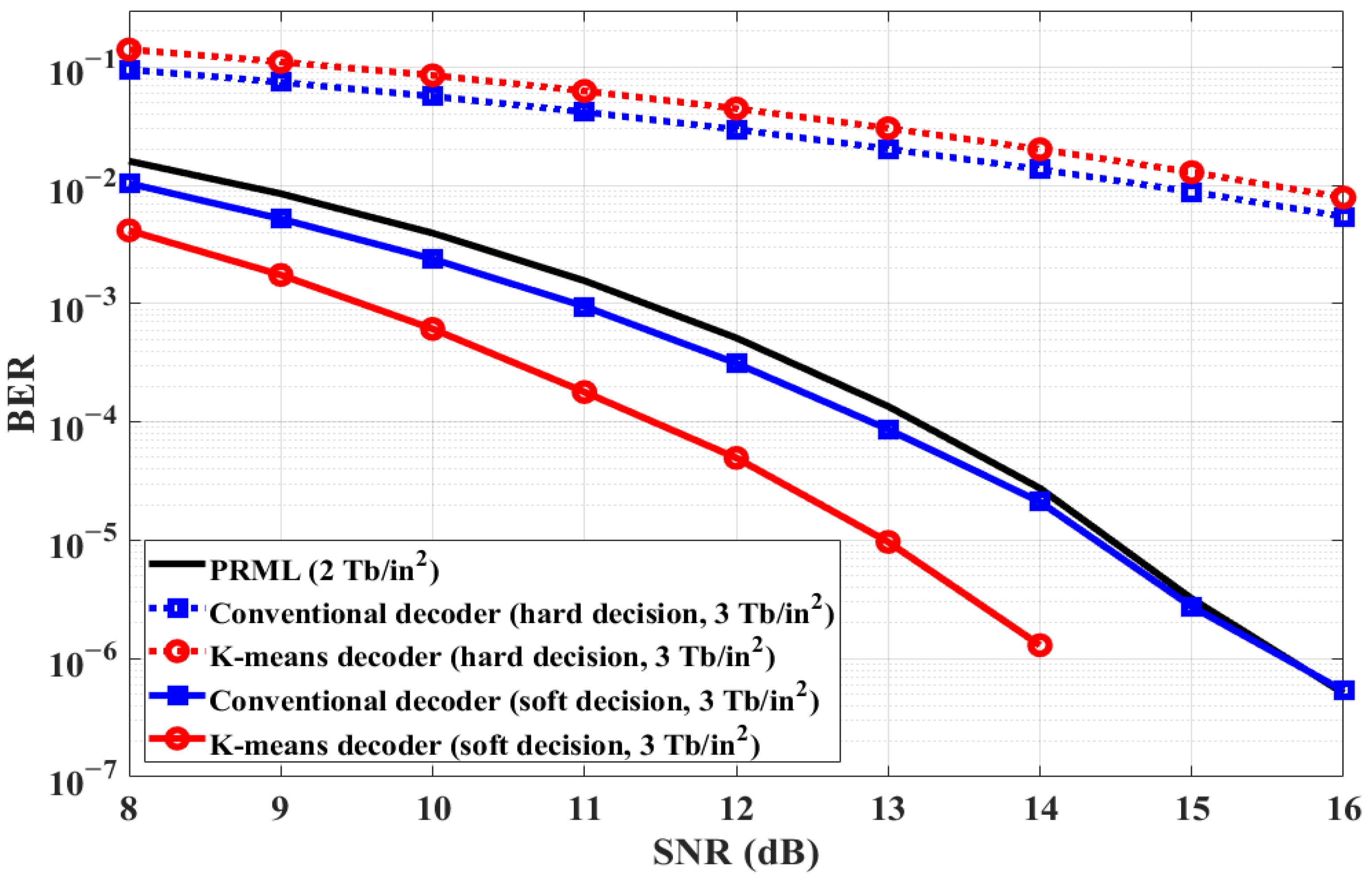
Figure 3 illustrates the BER performance of the decoding schemes according to SNR. The performance of the decoders using hard decisions is worse than that of the PRML detector. Since the hard decision detector determines a discrete or hard value (−1 or 1), where there are only two possible states, decoding loss occurs. Moreover, it is difficult to obtain the BER performance gain of the K-means decoder with hard decisions. However, the performances of the conventional and K-means decoder with soft decisions are 0.2 and 1.8 dB better than that of PRML at BER of 10−4, and the K-means decoder provides the best results.
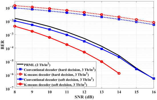
Figure 3.
BER performance of the decoding schemes according to SNR.
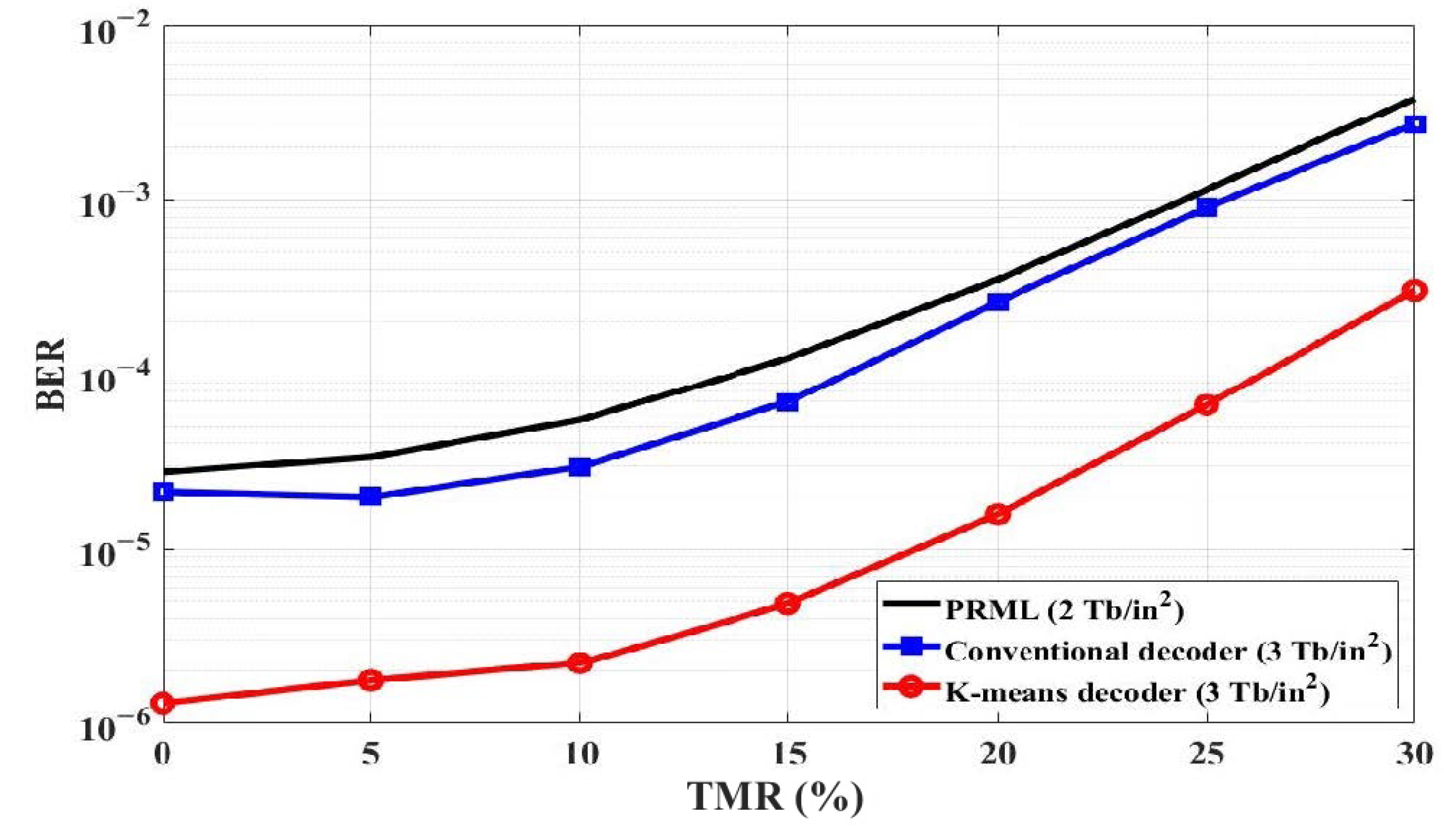
Figure 4 illustrates the BER performance of the decoding schemes in accordance with TMR at SNR of 14 dB. When the TMR is varied from 0% to 30%, the K-means decoder indicates better BER performance than the PRML detector and the conventional decoder.

Figure 4.
BER performance of the decoding schemes in accordance with TMR at SNR of 14 dB.
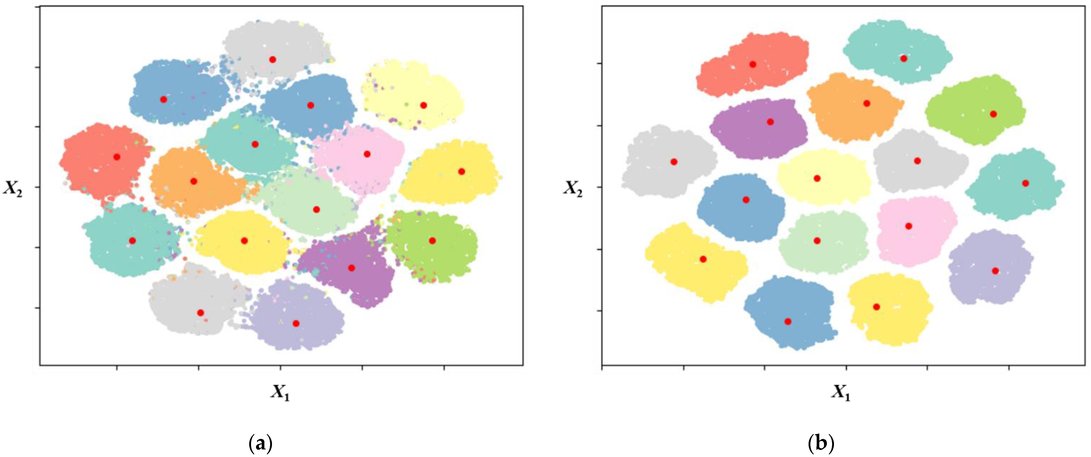
To verify why the performance of the K-means decoder is better than that of the conventional decoder, we explain the characteristics of the centroid using a scatter plot. Figure 5 displays the scatter plot of the received sequences from SOVA and the centroids at a SNR of 6 and 14 dB. Since it is difficult to visualize a dataset in a high-dimensional space, a dimensionality-reduction technique is needed to understand how the data are organized. Thus, to represent data visualization for the modulation code, we should reduce the dimensionality of the codeword from six to two dimensions. For dimensionality reduction, we use t-distributed stochastic neighbor embedding (t-SNE) [28]. t-SNE is a dimensionality-reduction technique that visualizes clusters of datasets in a high-dimensional space. It is useful to make similar datasets closer and dissimilar datasets further apart from each other. In Figure 5, there are 16 red points representing the centroids found by K-means and 16 clusters displayed as a collection of points because the number of codewords is 16. In Figure 5a, the points for each cluster are scattered due to noise or low SNR. However, as the SNR increases, as illustrated in Figure 5b, the points for each cluster are gathered. Further, the K-means algorithm can derive centroids from the received sequences and allocate them to an appropriate cluster.

Figure 5.
Scatter plot of the received sequences and centroids: (a) SNR = 6 dB; (b) SNR = 14 dB.
Table 3 lists the centroids of the K-means decoder based on hard and soft decisions at SNR = 14 dB. For the initialization of K-means, a codeword is used as the initial centroid. When using the hard decision, since the received sequence from the Viterbi detector is a hard-decision value and information loss occurs by the hard decision, the finalized centroid with a hard decision is also similar to the codeword. It is then difficult to achieve performance gain, as shown in Figure 3. However, when using the soft decision, since the received sequence from the SOVA detector is a soft-decision value, the K-means algorithm helps to understand data patterns and characteristics.
Table 3.
Centroids of K-means decoder according to hard and soft decision at SNR = 14 dB.
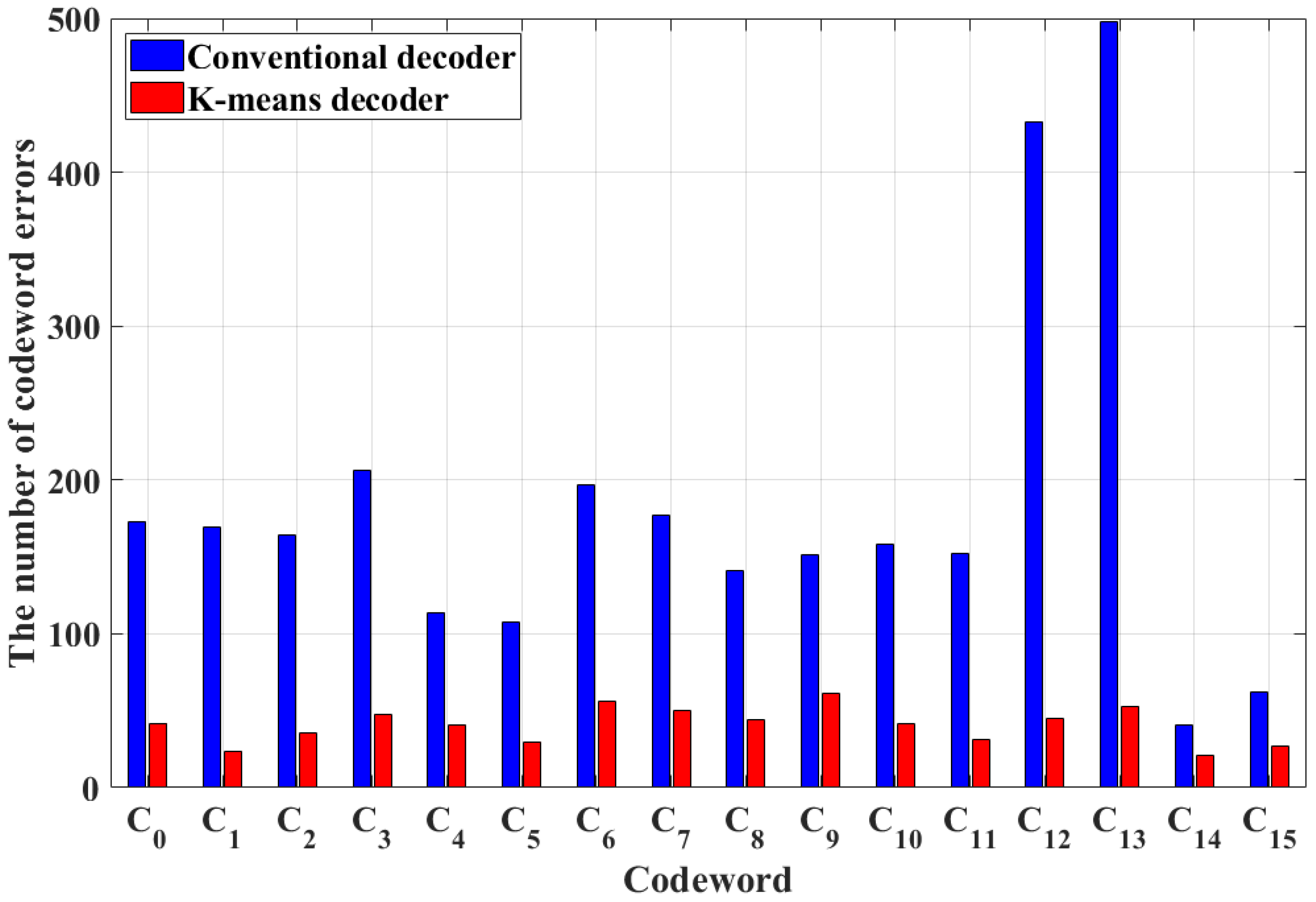
Figure 6 shows the number of codeword errors depending on the modulation decoding schemes when the SNR is 10 dB; in other words, when cl is transmitted by the encoder but the decoder determines ck (l ≠ k), the number of codeword errors for cl is counted. The total number of codeword errors in the conventional and K-means decoders is 2944 and 651, respectively. Additionally, when the conventional decoder is used, many codeword errors occur in C12 and C13 because the isolated patterns such as [−1, +1, −1]T and [+1, −1, +1]T can be generated by the adjacent neighboring codewords. However, when the K-means decoder is used, the number of errors in each codeword is similar because the K-means algorithm only considers data patterns and characteristics.
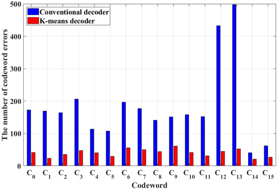
Figure 6.
The number of codeword errors depending on modulation decoding schemes when the SNR is 10 dB.
Consequently, it is difficult to obtain better BER performance using the conventional decoder and the K-means decoder with a hard decision. Thus, a soft decision is required to improve performance using modulation codes. The conventional decoder and the K-means decoder with soft decision performed better than the PRML detector at the same user density. The complexity of the K-means algorithm generally depends on the number of clusters and dimension. Therefore, when the number of codewords and the length of received sequence are increased, the complexity of the decoder based on the K-means algorithm is also increased, and this complexity is higher than that of the conventional decoder based on the Euclidean distance. However, since the original codewords are used to calculate Euclidean distance and the characteristics of data sequences are not fully considered in the conventional decoder, they show worse BER performance than the K-means decoder. Therefore, the K-means decoder with soft decision shows the best performance.
5. Conclusions
In this paper, we proposed a modulation decoding method based on the K-means algorithm for BPMR to improve decoding capabilities. In the conventional modulation decoder, the codeword is selected by a decoding algorithm using Euclidean distance. However, the elements of the original codewords consist only of −1 or +1, and the received sequences from SOVA are real-valued data. It is therefore difficult to consider the characteristics of the data sequences. To overcome the mismatch between the received sequence and codeword, we use the K-means algorithm for decoding, which helps to understand data patterns and characteristics. Further, to identify the data patterns and characteristics of the centroid, we show a scatter plot using the t-SNE technique, which is a dimensionality reduction technique. We verify that the K-means algorithm allocates the received sequences into an appropriate cluster and that the K-means decoder exhibits the best performance. Additionally, the K-means decoder is useful for improving the BER performance of the system when TMR occurs. Unlike signal processing schemes with long lists of rules by look-up table, signal processing schemes with machine learning would provide better solutions for complex problems which do not have a good solution using a traditional approach. Therefore, the modulation decoding scheme based on the K-means algorithm could be a good alternative. We will apply this scheme to other storage systems, such as holographic data storage systems, and study the detection and decoding schemes concatenated with the K-means or machine learning algorithm.
Author Contributions
S.J. contributed to this work in experiment planning, experiment measurements, data analysis and manuscript preparation; J.L. contributed to experiment planning, data analysis, and manuscript preparation. All authors have read and agreed to the published version of the manuscript.
Funding
This research was supported by the MSIT (Ministry of Science and ICT), Korea, under the ITRC (Information Technology Research Center) support program (IITP-2022-2020-0-01602) supervised by the IITP (Institute for Information & Communications Technology Planning & Evaluation).
Institutional Review Board Statement
Not applicable.
Informed Consent Statement
Not applicable.
Data Availability Statement
Not applicable.
Conflicts of Interest
The authors declare no conflict of interest.
References
- White, R.L.; New, R.M.H.; Pease, R.F.W. Patterned media: A viable route to 50 Gbit/in2 and up for magnetic recording. IEEE Trans. Magn. 1997, 33, 990–995. [Google Scholar]
- Richter, H.J.; Dobin, A.Y.; Heinonen, O.; Gao, K.Z.; Veerdonk, R.J.M.V.D.; Lynch, R.T.; Xue, J.; Weller, D.; Asselin, P.; Erden, M.F.; et al. Recording on bit-patterned media at densities of 1 Tb/in2 and beyond. IEEE Trans. Magn. 2006, 42, 2255–2260. [Google Scholar]
- Zhu, J.; Lin, Z.; Guan, L.; Messner, W. Recording, noise, and servo characteristics of patterned thin film media. IEEE Trans. Magn. 2000, 36, 23–29. [Google Scholar]
- Chang, W.; Cruz, J.R. Inter-track interference mitigation for bit-patterned magnetic recording. IEEE Trans. Magn. 2010, 46, 3899–3908. [Google Scholar]
- Yang, S.; Han, Y.; Wu, X.; Wood, R.; Galbraith, R. A soft decodable concatenated LDPC code. IEEE Trans. Magn. 2015, 51, 9401704. [Google Scholar]
- Keskinoz, M. Two-dimensional equalization/detection for patterned media storage. IEEE Trans. Magn. 2008, 44, 533–539. [Google Scholar]
- Nguyen, T.A.; Lee, J. Modified Viterbi algorithm with feedback using a two-dimensional 3-way generalized partial response target for bit-patterned media recording systems. Appl. Sci. 2021, 11, 728. [Google Scholar] [CrossRef]
- Jeong, S.; Lee, J. Iterative LDPC–LDPC product code for bit patterned media. IEEE Trans. Magn. 2017, 53, 3100704. [Google Scholar] [CrossRef]
- Jeong, S.; Lee, J. Modulation code for reducing intertrack interference on staggered bit-patterned media recording. Appl. Sci. 2020, 10, 5295. [Google Scholar] [CrossRef]
- Nguyen, T.A.; Lee, J. Error-correcting 5/6 modulation code for staggered bit-patterned media recording systems. IEEE Magn. Lett. 2019, 10, 6510005. [Google Scholar]
- Burse, K.; Yadav, R.; Shrivastava, S. Channel equalization using neural networks: A review. IEEE Trans. Syst. Man Cybern. Part C-Appl. Rev. 2010, 40, 352–357. [Google Scholar] [CrossRef]
- Cao, C.; Li, D.; Fair, I. Deep learning-based decoding of constrained sequence codes. IEEE J. Sel. Areas Commun. 2019, 37, 2532–2543. [Google Scholar] [CrossRef]
- Jeong, S.; Lee, J. Iterative signal detection scheme using multilayer perceptron for a bit-patterned media recording system. Appl. Sci. 2020, 10, 8819. [Google Scholar] [CrossRef]
- Jeong, S.; Lee, J. Bit-flipping scheme using k-means algorithm for bit-patterned media recording. IEEE Trans. Magn. 2022, 58, 3101704. [Google Scholar] [CrossRef]
- Jeong, S.; Lee, J. Modulation code and multilayer perceptron decoding for bit-patterned media recording. IEEE Magn. Lett. 2020, 11, 6502705. [Google Scholar] [CrossRef]
- Lloyd, S. Least squares quantization in PCM. IEEE Trans. Inf. Theory 1982, 28, 129–137. [Google Scholar] [CrossRef]
- Nabavi, S.; Kumar, B.V.K.V.; Bain, J.A. Two-dimensional pulse response and media noise modeling for bit-patterned media. IEEE Trans. Magn. 2008, 44, 3789–3792. [Google Scholar] [CrossRef]
- Nabavi, S.; Kumar, B.V.K.V.; Bain, J.A.; Hogg, C.; Majetich, S.A. Application of image processing to characterize patterning noise in self-assembled nano-masks for bit-patterned media. IEEE Trans. Magn. 2009, 45, 3523–3526. [Google Scholar] [CrossRef]
- Moon, J.; Zeng, W. Equalization for maximum likelihood detectors. IEEE Trans. Magn. 1995, 31, 1083–1088. [Google Scholar] [CrossRef]
- Ng, Y.; Cai, K.; Kumar, B.V.K.V.; Chong, T.C.; Zhang, S.; Chen, B.J. Channel modeling and equalizer design for staggered islands bit-patterned media recording. IEEE Trans. Magn. 2012, 48, 1976–1983. [Google Scholar] [CrossRef]
- Hagenauer, J.; Hoeher, P. A Viterbi algorithm with soft-decision outputs and its applications. In Proceedings of the 1989 IEEE Global Telecommunications Conference and Exhibition ‘Communications Technology for the 1990s and Beyond’, Dallas, TX, USA, 27–30 November 1989; pp. 1680–1686. [Google Scholar]
- Figueiredo, M.A.T.; Jain, A.K. Unsupervised learning of finite mixture models. IEEE Trans. Pattern Anal. Mach. Intell. 2002, 24, 381–396. [Google Scholar] [CrossRef]
- Krishna, K.; Narasimha Murty, M. Genetic K-means algorithm. IEEE Trans. Syst. Man Cybern. Part B-Cybern. 1999, 29, 433–439. [Google Scholar] [CrossRef] [PubMed]
- Sinaga, K.P.; Yang, M. Unsupervised K-Means Clustering Algorithm. IEEE Access 2020, 8, 80716–80727. [Google Scholar] [CrossRef]
- Na, S.; Xumin, L.; Yong, G. Research on K-means clustering algorithm: An improved K-means clustering algorithm. In Proceedings of the 2010 Third International Symposium on Intelligent Information Technology and Security Informatics, Ji’an, China, 2–4 April 2010; pp. 63–67. [Google Scholar]
- Scikit-Learn: Machine Learning in Phtyon. Available online: https://scikit-learn.org/stable/modules/clustering.html#k-means (accessed on 24 August 2022).
- Scikit-Learn: Machine Learning in Phtyon. Available online: https://scikit-learn.org/stable/modules/generated/sklearn.cluster.KMeans.html# (accessed on 24 August 2022).
- Maaten, L.v.d.; Hinton, G. Visualizing data using t-sne. J. Mach. Learn. Res. 2008, 9, 2579–2605. [Google Scholar]
Publisher’s Note: MDPI stays neutral with regard to jurisdictional claims in published maps and institutional affiliations. |
© 2022 by the authors. Licensee MDPI, Basel, Switzerland. This article is an open access article distributed under the terms and conditions of the Creative Commons Attribution (CC BY) license (https://creativecommons.org/licenses/by/4.0/).