Abstract
The propagation of infrasound in the atmosphere is influenced by atmospheric environmental parameters, which affect the precise localization of the infrasound source. Therefore, it has become crucial to quantify the influence of atmospheric environmental parameters on infrasound propagation. First, in this paper, the tau-p model is chosen as the physical model of infrasound propagation in a non-uniform moving medium. The atmospheric environmental parameters affecting infrasound propagation are determined. Secondly, the atmospheric environmental parameter distribution data are generated using the Sobol sampling method. Third, the generated atmospheric data are incorporated into the physical model of infrasound propagation to solve the output. Finally, Sobol sensitivity analysis is performed for each parameter, and the atmospheric parameter with the largest Sobol index is identified as the one with the most significant influence on infrasound propagation.
1. Introduction
Infrasound, or sound waves with frequencies below 20 Hz, is generated by human activities, including nuclear weapons tests and rocket launches as well as natural events such as earthquakes [1,2,3,4,5], volcanic eruptions [6,7,8,9], thunderstorms [10], and other geological disasters [11]. Infrasound is commonly used to monitor the occurrence of natural disasters such as volcanic eruptions, earthquakes, and mudslides. Infrasound is also used to precisely identify infrasound events through array signal processing algorithms. The use of infrasound is of great, practical importance for the monitoring and localization of infrasound events, especially natural disasters.
The propagation of infrasound in the atmosphere is easily disturbed by the propagation medium. The monitoring and location of infrasound events are affected by the changing atmospheric propagation medium. Therefore, it has become crucial to quantify the influence of atmospheric parameters on infrasound propagation. There are many uncertainties in infrasound propagation in the atmosphere, such as changes in temperature, atmospheric wind speed, and atmospheric density at different moments of the same location. The propagation trajectory of infrasound in a large-scale atmospheric environment are affected by these uncertainty factors because the atmospheric medium is a non-uniform medium with a non-uniform flow. The uncertain mechanism of infrasound propagation in complex atmospheric environments is analyzed to determine the parameters that have a greater influence on infrasound propagation. Quantifying the uncertainty of infrasound propagation can lay the foundation for the further realization of fast and accurate real-time localization of infrasound sources [12,13].
The most commonly used methods in uncertainty quantification are the Sobol sensitivity analysis [14,15,16,17,18] and Monte Carlo [19] and Latin hypercube sampling (LHS) [20]. The effect of input parameters on model output parameters can be quantified by the Sobol sensitivity analysis [21,22]. The method is applied to the uncertainty quantification of transient wave propagation in pressure pipelines [23] and to the uncertainty quantification analysis of sound source inversion methods [24]. The Sobol index method is based on the idea that the total variance and partial variance are used to express the effect of all variables on the output and the effect of univariate or multivariate analysis on the output, respectively. In the Sobol index method, the first-order Sobol index and the total Sobol index are usually used as sensitivity indicators for the input variables. The first indicator is the first-order Sobol index, which reflects the degree of contribution of a single input variable to the total variance of the model output and takes on values in the range of [0, 1]. The sensitivity of the input variables to the physical model can usually be ranked according to the value of the first-order Sobol index. A larger first-order Sobol index indicates that a change in that variable has a greater effect on the final output. The second indicator is the total Sobol index, which reflects the degree of influence of the main effects of the variables and the cross-effects of the variables with other variables on the model output variance. It takes on values in the range of [0, 1]. The total Sobol index contains the cross-effects of each variable. Supposing the value of the full-effects index of an input variable is small; this indicates that the change in the variable has a small impact on the change in the output, and the cross-effects between the variable and other variables also have a small impact on the output, i.e., the interaction effect between the two is also small. In the actual calculation, a certain number of variables can be reduced to simplify the computational model, but the variables must be those with a small total Sobol index.
The Sobol sensitivity analysis method is used to quantify the uncertainty of the parameters affecting infrasound propagation, to determine the parameters that have a decisive influence on infrasound propagation, and to reveal the mechanism generating infrasound propagation uncertainty. There are many kinds of uncertainty parameters in the atmosphere. The tau-p model [25,26,27,28,29], also known as the ray-tracing model [25], is used as a numerical simulation of infrasound propagation in a related paper. The atmospheric environmental parameters in this model can affect infrasound propagation. The sensitivity analysis of the atmospheric environmental parameters in the tau-p model is carried out using Sobol sensitivity analysis in order to rank the importance of the environmental parameters.
Therefore, the objective of this paper is to quantify the uncertain atmospheric environmental parameters that affect infrasound propagation in the atmosphere. The Sobol sensitivity-based approach is proposed to be able to rank the importance of uncertain atmospheric environmental parameters affecting infrasound propagation. First, the atmospheric parameters affecting infrasound propagation are identified in this paper. Secondly, the model of infrasound propagation in the atmosphere is determined. Finally, the importance ranking of the atmospheric parameters affecting infrasound propagation is performed using Sobol sensitivity analysis.
This paper is organized as follows. The infrasound propagation model is introduced in Section 2. The principles of Sobol sensitivity analysis and Sobol sequence are introduced in Section 3. The sensitivity analysis of the infrasound propagation model using data from the horizontal wind model (HWM93) and the mass spectrometer incoming scatter radar model (MSISE00) is presented in Section 4. Finally, conclusions are drawn in Section 5.
2. Physical Model of Infrasound Propagation
In the real atmospheric environment, the propagation speed of infrasound is affected by the wind speed . The type of wind affecting infrasound propagation can be classified into meridional wind and zonal wind . The effective sound velocity can be obtained by superimposing the wind velocity onto the sound speed c [30] at the receiving point. The effective sound velocity under the influence of wind speed is shown in Figure 1, and the effective sound velocity can be modeled as follows:
where is the specific heat ratio; T is the thermodynamic temperature; m is the atmospheric molar mass; R is the the universal gas constant equal to 8.314 /(); is the azimuth angle; is the unit vector along the direction of the wind speed .
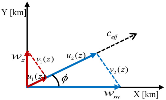
Figure 1.
Schematic diagram of effective sound velocity under wind speed. The X-axis indicates the meridional direction; Y-axis indicates the zonal direction. is the zonal wind; is the meridional wind. , and , are respectively the components of and along the direction of infrasound propagation and the components perpendicular to the direction of infrasound propagation.
In this paper, the tau-p model [28] is used to simulate the propagation process of infrasound in a moving atmospheric environment (effect of wind speed). The infrasound propagation distance, maximum height of infrasound propagation, and infrasound propagation time in a phase loop can be derived from the tau-p model.
The infrasound propagation distance R is the distance propagated from the bottom to the top of the atmospheric waveguide and then down the phase cycle. The specific formula is as follows:
while the corresponding travel time of a phase loop is
where is the surface altitude; is the maximum altitude of infrasound propagation. The transverse offset Q of the infrasound propagation model is calculated using the following equation:
where is the horizontal wind speed in the vertical propagation direction. The diagram of the infrasound propagation model is shown in part (a) of Figure 2. The model of infrasound propagation in the atmospheric environment is derived from the classical (Wentzel–Kramers–Brillouin–Jeffreys) [31] ray theory. When the horizontal phase velocity matches the effective sound velocity , the infrasound propagation ray will turn. Different infrasound propagation ray trajectories can be obtained by changing the elevation angle of the emission, as shown in part (b) of Figure 2.
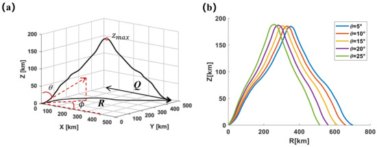
Figure 2.
(a) Propagation trajectory of the tau-p model in a phase loop. R represents the infrasound propagation distance of a phase loop in Equation (2); denotes the azimuth angle in Figure 1, indicates the angle of elevation; z represents the altitude of infrasound propagation; represents the maximum altitude that a phase loop can propagate; Q represents the lateral offset of infrasound propagation in Equation (4). (b) Infrasound propagation trajectories at different elevation angles in a phase loop. z denotes altitude; the angle values are from 5 to 25 at intervals of 5.
Each ray is represented by an invariant ray parameter p. When considering the influence of wind speed, the corresponding ray parameter p is calculated as follows:
where is the speed of sound for an unperturbed fluid at the receiving point, i.e., the sound velocity not influenced by the wind speed; is the horizontal wind speed along the direction of infrasound propagation at an altitude of 0; is the elevation angle of the emission in Figure 2.
is the characteristic function, and it is expressed as follows:
where the root of the characteristic function corresponds to the ray turning point, i.e., the height of the turning point is . The in Equation (2) is the first root above of the characteristic function.
It is evident from the tau-p model that infrasound is susceptible to the influence of atmospheric physical parameters during propagation. Determining the source of uncertainty and quantifying its effect on infrasound propagation is thus an important issue.
3. Sobol Index for Sensitivity Analysis of the Tau-p Model
3.1. Sobol Sequence Mathematical Principle
The Sobol sequence is a sequence using the minimum prime number 2 as the base in order to generate a random sequence . First, an integrable polynomial S with a base of 2 (highest order n) is used to generate the direction numbers of n. The original polynomial is
The direction numbers are
where , , ⋯, . It has the following relationship with the sequence , , :
where ⊕ is the bit-by-bit exclusive-or operator; is an arbitrary positive integer satisfying the odd integer ; and n, , , ⋯, , , , are initially given, i.e., are initially calculated. If the number of desired directions is greater than q, then
Therefore, the random number generated by the Sobol sequence is as follows:
The Sobol sequences in the unit hypercube [0,1] with n ≤ 40 can be generated based on the Sobol sequence mathematical principle, whose two-dimensional schematic is shown in Figure 3.
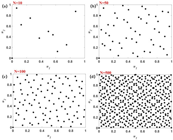
Figure 3.
Graphs (a–d) represent the sampling numbers of 10, 50, 100, 500 two-dimensional Sobol sampling schematics, respectively. , are two parameters in the range [0–1].
3.2. Mathematical Principles of Sobol Sensitivity Analysis
The theory of variance-based Sobol sensitivity indices [15] is introduced in this section. The Sobol sensitivity analysis is achieved based on the quasi-Monte Carlo (QMC) [17]. The first-order Sobol index and the total Sobol index are calculated by this method to estimate the effect of individual variables or groups of variables on the model output. Given samples of , let represent the output computed from the infrasound physical model (tau-p model):
where () denotes the m-th atmospheric environmental parameter. The mean value of the tau-p model output is as follows:
The total variance can be calculated by the following equation:
Similarly, the first-order Sobol index for the m-th uncertain atmospheric environmental parameter is calculated as follows:
where is the partial variance. It can be obtained by the following equation:
where and are two independent Sobol sample sets from . The format of the sample set is a matrix of , where M denotes the number of uncertain atmospheric environmental parameter types. is the m-th column of the first sample set replaced by the mth column of the second sample set . denotes the set of all variables except , and Var denotes the variance symbol. denotes the mathematical expectation symbol. The second-order Sobol index can be obtained by the following equation:
which describes the mutual cross-effects of uncertain atmospheric parameters -th and -th on the tau-p model output , in which
Then, the total Sobol index [16,17] is calculated as follows:
which describes the extent to which the cross-effect of the uncertain atmospheric parameter m-th with other atmospheric parameters affects the output of the tau-p model. With the increase of uncertain parameters M, it is necessary to calculate the Sobol index. To simplify the calculation, the total Sobl index is approximated as follows [17]:
3.3. Pseudocode for Tau-p Model Sensitivity Analysis
First, the atmospheric parameter reference data with altitude z distribution are imported. A polynomial curve is fitted to the atmospheric background reference data. The maximum sampling Sobol number is set, and the polynomial curve fitting coefficients are sampled to generate the atmospheric background data. The atmospheric background data are substituted into the tau-p model to calculate the corresponding output. Finally, the first-order Sobol index and the total Sobol index that correspond to each atmospheric parameter are calculated. For example, the pseudocode for analyzing the influence of the infrasound propagation distance R is shown in Algorithm 1. In this paper, the degree of influence of atmospheric physical parameters on infrasound propagation distance R, maximum propagation height , and travel time t are analyzed separately. The corresponding sensitivity indices of each parameter are determined.
| Algorithm 1: Pseudocode for tau-p model sensitivity analysis. |
| Input: , ; |
| Output: , ; |
| 1: initialize: ; |
| 2: while ; |
| 3: Compute: R using Equation (2) |
| 4: Compute: using Equation (15) |
| 5: Compute: using Equation (20) |
| 6: |
| 7: end |
3.4. Flow Chart of Uncertainty Quantification Technique for the Infrasound Propagation Model
The first step obtains the reference data of atmospheric background parameters with height distribution from the MSISE00 and HWM93 models. In the second step, the distribution curves of the atmospheric background parameters are generated based on the Sobol series sampling of the reference data. The criterion for the generated atmospheric physical parameter distribution curves is to make the atmospheric parameter distribution curves conform to the actual distribution and not deviate from the reference value. In the third step, the sensitivity analysis of atmospheric background parameters is performed using Sobol sensitivity analysis. The first-order sensitivity and total Sobol index corresponding to each atmospheric background parameter are calculated. The technical flowchart of this paper is shown in Figure 4.
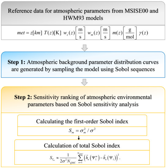
Figure 4.
In the first step, the reference data of the atmospheric background parameters with height distribution are obtained from the MSISE00 and HWM93 models. In the second step, the distribution curves of atmospheric background parameters are generated based on the Sobol series sampling of the reference data. In the third step, the sensitivity analysis of atmospheric background parameters is performed using Sobol sensitivity analysis, and the first-order sensitivity index and total Sobol index corresponding to each atmospheric background parameter are calculated.
4. Quantitative Results Presentation and Analysis Based on the Actual Atmospheric Data
4.1. Sobol Sampling to Generate Atmospheric Profile Curves
The Sobol index method is used to analyze the atmospheric physical parameters affecting infrasound propagation. After observing the infrasound propagation model, thermodynamic temperature, zonal wind, meridional wind, mean atmospheric molar mass, and specific heat ratio are identified as the physical parameters that may affect the atmospheric propagation. The atmospheric physical parameters are in the altitude range of 1–200 km, and 1000 points can be acquired at an altitude interval of = 0.2 km. The baseline parameter curves for the above physical parameters are selected, i.e., the curves of the atmospheric physical parameter values with height (source of baseline parameter data: MSISE00 and HWM93 models). The format of the atmospheric background data is as follows:
where T is the temperature; is the zonal wind speed; is the meridional wind speed; m is the average molar mass of the atmosphere; is the specific heat ratio. The magnitudes of T, , , m are (K), (m/s), (m/s), (g/mol), respectively. The baseline parameter curves are fitted using polynomial curve fitting in order to obtain the fitted coefficient values of the baseline curves. The sampling interval of the fitting coefficient is obtained by adjusting the sampling range of the fitting coefficient so that the distribution curve generated after sampling will conform to the actual atmospheric environment. The range of values of the curve fitting coefficients are uniformly distributed. The polynomial expansion of the five atmospheric parameters is shown in Equation (22).

Table 1.
The range of values of the polynomial curve fitting coefficients for the five atmospheric parameters.
The number of samples for the curve fitting coefficients is set to 1200. The sampled atmospheric parameter distribution curves are plotted in a graph, as shown in Figure 5. The black line represents the reference atmospheric parameter distribution curve, and the red line represents the generated atmospheric parameter distribution curve after sampling.
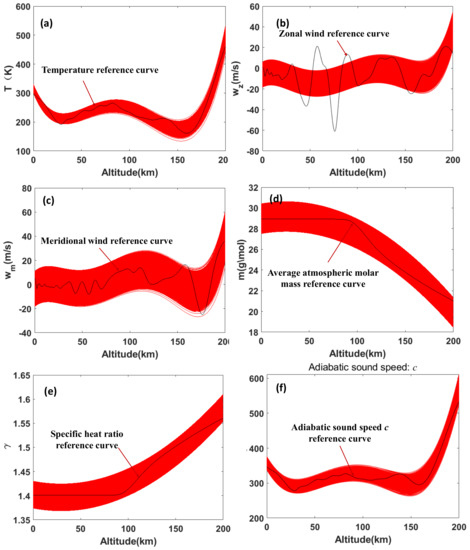
Figure 5.
Distribution curves of each atmospheric parameter generated after Sobol sampling (the number of sampling is 1200). The black line represents the reference atmospheric parameter distribution curve, and the red line represents the atmospheric parameter distribution curve generated after sampling. Graphs (a–f) illustrate temperature T, zonal wind speed , meridional wind speed , average atmospheric molar mass m, specific heat ratio , and adiabatic sound speed c, respectively (Data from: https://kauai.ccmc.gsfc.nasa.gov/instantrun/msis, accessed on 15 May 2021).
From Figure 5, it can be seen that the fitted parameter curves are well-distributed at a reasonable interval without exceeding the real atmospheric environment. Therefore, the fitted atmospheric parameter distribution data can be imported as input data into the tau-p model in order to solve for the output.
4.2. Uncertainty Quantification Analysis for the Infrasound Propagation Distance
The sampled parameter profiles are imported into the tau-p model as atmospheric background parameters to calculate the corresponding outputs. In this paper, the infrasound propagation distance R is selected as the output of the infrasound propagation physical model. The source position of the tau-p model is set to the ground at an altitude of 0; the elevation angle of the emission angle is set to a fixed value of 30°; the azimuth angle is 45°. The first-order sensitivity index and the total Sobol index of each parameter are solved by the Sobol index method. These two indices can reflect the degree of influence of the atmospheric parameters on the physical model of infrasound propagation. The first-order Sobol index convergence curves and the total Sobol index convergence curves for the five atmospheric parameters are shown in (a) and (b) of Figure 6, respectively. The range of Sobol sampling times N is from 500 to 3000.
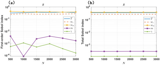
Figure 6.
(a) Five atmospheric parameters’ first-order Sobol index convergence lines for the infrasound propagation distance R; (b) Five atmospheric parameters’ total Sobol index convergence lines for the infrasound propagation distance R (the blue, dark red, yellow, purple, and light green curves indicate temperature T, zonal wind , meridional wind , mean atmospheric molar mass m, and specific heat ratio , respectively).
It can be seen from Figure 6 that with the increase of sampling times, the first-order Sobol index and total Sobol index of each atmospheric parameter converge. The first-order Sobol index and the total Sobol index when the number of Sobol samples is 2000 are shown in Figure 7. The specific values of the two indices are shown in Table 2.
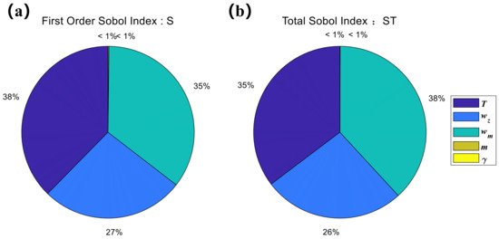
Figure 7.
(a) First-order Sobol index pie charts and (b) total Sobol index pie charts of the five parameters for the infrasound propagation distance R. The five uncertain atmospheric environmental parameters are independently and uniformly distributed. The number of Sobol samples N is 2000.
Table 2.
First Sobol index S and Total Sobol index ST of each atmospheric parameter for the infrasound propagation distance R.
It can be seen in Table 2 that the parameters that have a great impact on infrasound propagation distance have been sorted as follows:
(1) The first-order impact indices in descending order are meridional wind, thermodynamic temperature, zonal wind, mean atmospheric molar mass, and specific heat ratio;
(2) The order of the total impact indices from the largest to the smallest is as follows: meridional wind, thermodynamic temperature, zonal wind, mean atmospheric molar mass, and specific heat ratio. It can be seen that the atmospheric environmental parameter with the greatest influence on the infrasound propagation distance is the meridional wind from these two sensitivity indices.
In the non-uniform atmospheric environment, the infrasound propagation distance R is mainly related to the infrasound propagation velocity, i.e., the effective sound velocity. From the effective sound velocity model in Equation (1), it can be seen that the zonal wind and the meridional wind are the main parameters affecting the effective sound velocity. The atmospheric temperature is weakened by taking the root sign, which leads to the effect on the effective sound velocity. The wind speed in the latitudinal direction after sampling is (−27.64 m/s, 53.81 m/s), i.e., the interval length is 81.45 m/s. The wind speed in the meridional direction after sampling is (−26.80 m/s, 60.05 m/s), i.e., the interval length is 86.85 m/s. Therefore, it can be inferred that the influence of the meridional wind on the infrasound propagation distance R is greater than that of the zonal wind. This conclusion needs to combine the data of zonal and meridional winds in a specific area and time, and it is not generalizable.
4.3. Uncertainty Quantification Analysis for the Maximum Height of Infrasound Propagation
The sensitivity analysis of the atmospheric physical parameters affecting the maximum propagation height of infrasound is performed using the Sobol sensitivity analysis method. The maximum propagation distance is chosen as the output of the tau-p model. The source position of the tau-p model is set to the ground at an altitude of 0; the ray emission angle is set to a fixed value of 30°; the azimuth angle is 20°. The first-order Sobol index convergence curves and the total Sobol index convergence curves for each atmospheric parameter are shown in (a) and (b) of Figure 8, respectively. The range of Sobol sampling times N is from 500 to 5000.
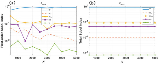
Figure 8.
(a) Five atmospheric parameters’ first-order Sobol index convergence lines for the maximum height of infrasound propagation ; (b) Five atmospheric parameters’ total Sobol index convergence lines for the maximum height of infrasound propagation (the blue, dark red, yellow, purple, and light green curves indicate temperature T, zonal wind , meridional wind , mean atmospheric molar mass m, and specific heat ratio , respectively).
It can be seen from the above figures that the two indices tend to converge as the sampling times increase. The results of the first-order Sobol index and the total Sobol (5000 Sobol samples) for each atmospheric physical parameter are plotted in Figure 9. The sensitivity index values corresponding to the degree of influence of each atmospheric physical parameter on the maximum height of infrasound propagation are shown in Table 3.
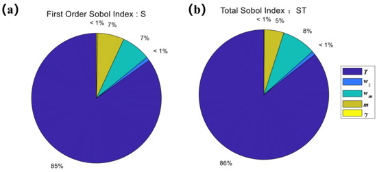
Figure 9.
(a) First-order Sobol index pie charts and (b) total Sobol index pie charts of the five parameters for the infrasound propagation maximum height. The five uncertain atmospheric environmental parameters are independently and uniformly distributed. The number of Sobol samples N is 5000.
Table 3.
First Sobol index S and Total Sobol index ST of each atmospheric parameter for the infrasound propagation maximum height.
In Table 3, it can be seen that the parameters that have a large influence on the maximum height of infrasound propagation have been ranked as follows:
(1) The first-order influence indices in descending order are the thermodynamic temperature, meridional wind, mean atmospheric molar mass, zonal wind, and specific heat ratio;
(2) The total impact indices in descending order are the thermodynamic temperature, meridional wind, mean atmospheric molar mass, zonal wind, and specific heat ratio. From these two sensitivity indices, it can be seen that the atmospheric environmental parameter with the greatest influence on the infrasound propagation distance is the thermodynamic temperature.
The maximum height of infrasound propagation is mainly influenced by the infrasound propagation velocity in the direction perpendicular to the ground. It can be seen in Figure 2 that the component of infrasound propagation velocity perpendicular to the ground is , where . Through Equation (1), it can be seen that temperature can affect the velocity of infrasound propagation in the vertical ground direction, ultimately affecting the maximum height of infrasound propagation. The zonal and meridional winds in this paper are horizontal winds, which mainly affect the propagation distance of infrasound in the horizontal direction. It has little effect on the maximum height of infrasound propagation.
4.4. Uncertainty Quantification Analysis for the Travel Time of Infrasound Propagation on a Phase Loop
The Sobol sensitivity analysis is used to quantify and analyze the main atmospheric physical parameters that affect the travel time on a phase loop. In this paper, atmospheric temperature, meridional wind, zonal wind, mean atmospheric molar mass, and specific heat ratio are selected as the atmospheric physical parameters to be quantified. The travel time of the tau-p model is chosen as the output. The source position of the tau-p model is set to the ground at an altitude of 0; the elevation angle of emission is set to a fixed value of 30°; the azimuth angle is 20°. The convergence curves of the first-order Sobol sensitivity index S and the total Sobol index are plotted in (a) and (b) of Figure 10, respectively. The range of Sobol sampling times N is from 200 to 2400.
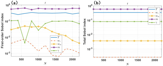
Figure 10.
(a) Five atmospheric parameters’ first-order Sobol index convergence lines for the infrasound propagation travel time t in a phase loop; (b) Five atmospheric parameters’ total Sobol index convergence lines for the infrasound propagation travel time t in a phase loop (the blue, dark red, yellow, purple, and light green curves indicate temperature T, zonal wind , meridional wind , mean atmospheric molar mass m, and specific heat ratio , respectively).
It can be seen that the two indices converge as the number of Sobol samples increases. The results with a sampling number of 2400 were chosen, and pie charts of the first-order Sobol index and the total Sobol index were drawn separately, as shown in Figure 11. The sensitivity index values corresponding to the degree of influence of each atmospheric physical parameter on the infrasound propagation travel time in a phase loop are shown in Table 4.
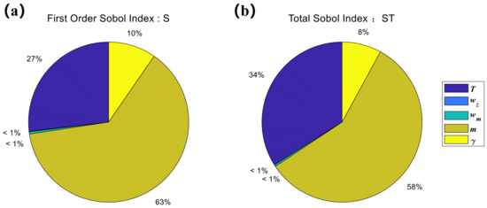
Figure 11.
(a) First-order Sobol index pie charts and (b) total Sobol index pie charts representing the five parameters for travel time t. The five uncertain atmospheric environmental parameters are independently and uniformly distributed. The number of Sobol samples N is 2400.
Table 4.
First-order Sobol index S and total Sobol index of each atmospheric parameter for infrasound propagation travel time in a phase loop.
In Table 4, it can be seen that the parameters that have a large influence on the travel time of infrasound propagation have been ranked as follows:
(1) The first-order influence indices in descending order are the mean atmospheric molar mass, specific heat ratio, thermodynamic temperature, meridional wind, and zonal wind;
(2) The total impact indices in descending order are the mean atmospheric molar mass, specific heat ratio, thermodynamic temperature, meridional wind, and zonal wind.
From these two sensitivity indices, it can be seen that the atmospheric environmental parameter with the greatest influence on the infrasound propagation travel time is the mean atmospheric molar mass. From the term of Equation (3), it can be seen that the atmospheric molar mass, as the numerator term, ranges from 18.45 g/mol to 30.62 g/mol after sampling. The atmospheric temperature and specific heat ratio as the denominator term parameters after sampling fall within the ranges of (134.06 K, 532.73 K) and (1.37, 1.61), respectively. The change as the numerator term has a more significant effect on the infrasound propagation time t than the change in the denominator term. Therefore, it can be inferred from Equation (3) that the main atmospheric parameter affecting the infrasound propagation time is the average atmospheric molar mass. As shown in Figure 5 (d), the average atmospheric molar mass m is almost constant below 100 km. This conclusion applies especially to rays propagating beyond an altitude of 100 km.
The conclusions in this paper are drawn under the MSISE00 model and the HWM93 model, i.e., the three conclusions above are based on region-specific atmospheric data. Therefore, the above conclusions are not generalizable. This paper provides a method of quantifying the uncertainty of infrasound propagation for a specific region. For a specific region, the uncertainty quantification of infrasound propagation needs to be performed based on the acquisition of region-specific atmospheric data. The results of the above study can further understand the propagation law of infrasound, reveal the mechanism of infrasound propagation, and lay the foundation for further localization of infrasound sources in uncertain atmospheric environments. The uncertainty information of infrasound propagation can be incorporated into the Bayesian framework as a priori knowledge [32,33]. In addition, infrasound source localization algorithms in a Bayesian framework have been developed [34]. Therefore, by combining the above two points, the uncertainty information of the infrasound propagation environment can be incorporated into the infrasound source localization algorithm to achieve enhanced localization results in the future. The nonlinear effect of the infrasound propagation process is not considered by the tau-p model. Considering the nonlinear effects of the infrasound propagation process can better reflect the real infrasound propagation process in the atmosphere [35,36]. Future work on the quantification of infrasound propagation uncertainty should aim to consider the nonlinear effects of the infrasound propagation process.
5. Conclusions
The uncertainty quantification method of the infrasound propagation model was implemented. Uncertain parameters (thermodynamic temperature, meridional wind, zonal wind, mean atmospheric molar mass, specific heat ratio) that affect infrasound propagation in complex atmospheric environments were considered. The sensitivity of the uncertain parameters to infrasound propagation was studied. The results show that the parameter that has a decisive influence on the propagation distance of infrasound is the meridional wind. The thermodynamic temperature is the parameter that has a decisive influence on the maximum height of infrasound propagation. The parameter that has a decisive influence on the infrasound travel time is the mean atmospheric molar mass. The above three conclusions are based on the MSISE00 model and the HWM93 model. The above uncertainty quantification analysis results are useful for the further understanding of the mechanisms of infrasound propagation in the atmosphere. They can also serve as data reference for infrasound source localization under an uncertain atmospheric environment. This paper analyzed the effects of five atmospheric parameters on infrasound propagation. In the future, the uncertainty quantification results can be modeled into the infrasound source localization algorithm as a priori information in order to enhance the localization effect.
Author Contributions
Conceptualization, R.W. and L.Y.; methodology, R.W., L.Y., X.Y. and C.Z.; formal analysis, X.Y.; data curation, X.Y.; software, X.Y. and C.Z.; writing— original draft, X.Y., R.W., L.Y., C.Z., T.W. and X.Z.; writing—review and editing, R.W., L.Y., C.Z., T.W. and X.Z.; supervision, R.W. and L.Y.; funding acquisition, R.W. and L.Y. All authors have read and agreed to the published version of the manuscript.
Funding
This work was supported by the Open Fund of State Key Laboratory of Mechanical Transmissions of Chongqing University, China (SKLMT-MSKFKT202015), the National Natural Science Foundation of China (Grant Nos. 12074254 and 51505277), the Natural Science Foundation of Shanghai (Grant No. 21ZR1434100), and the Open Fund of the Key Laboratory of Aerodynamic Noise Control (ANCL20210301). This work was also sponsored by the Oceanic Interdisciplinary Program of Shanghai Jiao Tong University (Project No. SL2021MS009).
Institutional Review Board Statement
Not applicable.
Informed Consent Statement
Not applicable.
Data Availability Statement
Measured wind data from Los Alamos National Laboratory (https://www.lanl.gov/org/ddste/aldcels/earth-environmental-sciences/geophysics/software/seismoacoustics/inframonitor.php, accessed on 15 May 2021). Average atmospheric molar mass, specific heat ratio, and temperature data were obtained from the MSISE00 model (https://kauai.ccmc.gsfc.nasa.gov/instantrun/msis, accessed on 15 May 2021).
Acknowledgments
The authors would like to thank Xun Wang (Beihang University) for his support and full discussion. We thank Los Alamos National Laboratory for providing the wind data. We thank the Community Coordinated Modeling Center (CCMC) for providing the data for atmospheric temperature, atmospheric molar mass, and specific heat ratio.
Conflicts of Interest
The authors declare no conflict of interest.
Abbreviations
The following abbreviations are used in this manuscript:
| c | static sound speed at the receiving point |
| unit vector along the direction of wind speed | |
| wind speed along the direction of infrasound propagation | |
| meridional wind | |
| zonal wind | |
| specific heat ratio | |
| T | thermodynamic temperature |
| m | atmospheric molar mass |
| R | universal gas constant |
| azimuth angle | |
| elevation angle of emission | |
| z | altitude |
| surface altitude | |
| maximum altitude of infrasound propagation | |
| characteristic function | |
| p | ray parameter |
| output computed from the infrasound physical model (tau-p model) | |
| vector of uncertain parameters | |
| () | m-th atmospheric environmental parameter |
| partial variance | |
| independent Sobol sample sets from | |
| first-order Sobol index for the m-th uncertain atmospheric environmental | |
| parameter | |
| Var | variance symbol |
| mathematical expectation symbol | |
| second-order Sobol index | |
| set of all variables except | |
| total Sobol index |
References
- Raspet, R.; Hickey, C.J.; Koirala, B. Corrected Tilt Calculation for Atmospheric Pressure-Induced Seismic Noise. Appl. Sci. 2022, 12, 1247. [Google Scholar] [CrossRef]
- Lu, J.; Wang, Y.; Chen, J. Noise Attenuation Based on Wave Vector Characteristics. Appl. Sci. 2018, 8, 672. [Google Scholar] [CrossRef]
- Gonzalez, A.; Calderon, J. An Overview of the Seismic Elastic Response Spectra and Their Application According to Mexican, U.S., and International Building Codes. Appl. Sci. 2022, 12, 3472. [Google Scholar] [CrossRef]
- Li, J.; He, M.; Cui, G.; Wang, X.; Wang, W.; Wang, J. A Novel Method of Seismic Signal Detection Using Waveform Features. Appl. Sci. 2020, 10, 2919. [Google Scholar] [CrossRef]
- Mutschlecner, P.J.; Whitaker, R.W. Infrasound from earthquakes. J. Geophys. Res. Atmos. 2005, 110, D01108. [Google Scholar] [CrossRef]
- Freret-Lorgeril, V.; Bonadonna, C.; Corradini, S.; Donnadieu, F.; Guerrieri, L.; Lacanna, G.; Marzano, F.S.; Mereu, L.; Merucci, L.; Ripepe, M.; et al. Examples of Multi-Sensor Determination of Eruptive Source Parameters of Explosive Events at Mount Etna. Remote Sens. 2021, 13, 2097. [Google Scholar] [CrossRef]
- Cigna, F.; Tapete, D.; Lu, Z. Remote Sensing of Volcanic Processes and Risk. Remote Sens. 2020, 12, 2567. [Google Scholar] [CrossRef]
- Batubara, M.; Yamamoto, M.y. Infrasound Observations of Atmospheric Disturbances Due to a Sequence of Explosive Eruptions at Mt. Shinmoedake in Japan on March 2018. Remote Sens. 2020, 12, 728. [Google Scholar] [CrossRef]
- De Angelis, S.; Diaz-Moreno, A.; Zuccarello, L. Recent Developments and Applications of Acoustic Infrasound to Monitor Volcanic Emissions. Remote Sens. 2019, 11, 1302. [Google Scholar] [CrossRef]
- Le Pichon, A.; Blanc, E.; Hauchecorne, A. Infrasound Monitoring for Atmospheric Studies; Springer Science & Business Media: Berlin/Heidelbeg, Germany, 2010. [Google Scholar]
- Schimmel, A.; Hübl, J. Automatic detection of debris flows and debris floods based on a combination of infrasound and seismic signals. Landslides 2016, 13, 1181–1196. [Google Scholar] [CrossRef]
- Modrak, R.T.; Arrowsmith, S.J.; Anderson, D.N. A Bayesian framework for infrasound location. Geophys. J. Int. 2010, 181, 399–405. [Google Scholar] [CrossRef]
- Blom, P.S.; Marcillo, O.; Arrowsmith, S.J. Improved Bayesian Infrasonic Source Localization for regional infrasound. Geophys. J. Int. 2015, 203, 1682–1693. [Google Scholar] [CrossRef]
- Sobol, I.M. On the distribution of points in a cube and the approximate evaluation of integrals. Zhurnal Vychislitel’noi Matematiki i Matematicheskoi Fiziki 1967, 7, 784–802. [Google Scholar] [CrossRef]
- Sobol, I.M. Sensitivity estimates for nonlinear mathematical models. Math. Model. Comput. Exp. 1993, 1, 407–414. [Google Scholar]
- Sobol, I.M. On sensitivity estimation for nonlinear mathematical models. Mat. Model. 1990, 2, 112–118. [Google Scholar]
- Sobol, I. Global sensitivity indices for nonlinear mathematical models and their Monte Carlo estimates. Math. Comput. Simul. 2001, 55, 271–280. [Google Scholar] [CrossRef]
- Zhuang, Y.; Luo, S.; Easa, S.M.; Zhang, M.; Wang, C. Mechanical Performance of Curved Link-Slab of Simply Supported Bridge Beam. Appl. Sci. 2022, 12, 3344. [Google Scholar] [CrossRef]
- Evans, M.; Swartz, T. Approximating Integrals via Monte Carlo and Deterministic Methods; OUP Oxford: Oxford, UK, 2000; Volume 20. [Google Scholar]
- Wilson, D.K.; Pettit, C.L.; Ostashev, V.E.; Vecherin, S.N. Description and quantification of uncertainty in outdoor sound propagation calculations. J. Acoust. Soc. Am. 2014, 136, 1013–1028. [Google Scholar] [CrossRef]
- Prikaziuk, E.; van der Tol, C. Global Sensitivity Analysis of the SCOPE Model in Sentinel-3 Bands: Thermal Domain Focus. Remote Sens. 2019, 11, 2424. [Google Scholar] [CrossRef]
- Morcillo-Pallarés, P.; Rivera-Caicedo, J.P.; Belda, S.; De Grave, C.; Burriel, H.; Moreno, J.; Verrelst, J. Quantifying the Robustness of Vegetation Indices through Global Sensitivity Analysis of Homogeneous and Forest Leaf-Canopy Radiative Transfer Models. Remote Sens. 2019, 11, 2418. [Google Scholar] [CrossRef]
- Wang, X. Uncertainty Quantification and Global Sensitivity Analysis for Transient Wave Propagation in Pressurized Pipes. Water Resour. Res. 2021, 57, e2020WR028975. [Google Scholar] [CrossRef]
- Gilquin, L.; Bouley, S.; Antoni, J.; Le Magueresse, T.; Marteau, C. Sensitivity analysis of two inverse methods: Conventional beamforming and Bayesian focusing. J. Sound Vib. 2019, 455, 188–202. [Google Scholar] [CrossRef]
- Garcés, M.A.; Hansen, R.A.; Lindquist, K.G. Traveltimes for infrasonic waves propagating in a stratified atmosphere. Geophys. J. Int. 1998, 135, 255–263. [Google Scholar] [CrossRef]
- Jones, R.M.; Gu, E.S.; Bedard, A., Jr. Infrasonic Atmospheric Propagation Studies Using a 3-D Ray Trace Model. In Preprints, 22nd Conf. on Severe Local Storms, Hyannis, MA, USA, Meteor. Soc. P. Citeseer. 2004, Volume 2. Available online: https://cires1.colorado.edu/events/rendezvous/2007/posters/I3B.pdf (accessed on 10 May 2021).
- Lonzaga, J.; Waxler, R.; Assink, J.; Talmadge, C. Modelling waveforms of infrasound arrivals from impulsive sources using weakly non-linear ray theory. Geophys. J. Int. 2015, 200, 1347–1361. [Google Scholar] [CrossRef][Green Version]
- Drob, D.P.; Garcés, M.; Hedlin, M.; Brachet, N. The temporal morphology of infrasound propagation. Pure Appl. Geophys. 2010, 167, 437–453. [Google Scholar] [CrossRef]
- Arrowsmith, S.J.; Whitaker, R.; Taylor, S.R.; Burlacu, R.; Stump, B.; Hedlin, M.; Randall, G.; Hayward, C.; ReVelle, D. Regional monitoring of infrasound events using multiple arrays: Application to Utah and Washington State. Geophys. J. Int. 2008, 175, 291–300. [Google Scholar] [CrossRef]
- Shang, C.; Teng, P.; Lyu, J.; Yang, J.; Sun, H. Infrasonic source altitude localization based on an infrasound ray tracing propagation model. J. Acoust. Soc. Am. 2019, 145, 3805. [Google Scholar] [CrossRef] [PubMed]
- Landau, L.; Lifshitz, E. The Classical Theory of Fields; Addison-Wesley: Cambridge, UK, 1951. [Google Scholar]
- Antoni, J. A Bayesian approach to sound source reconstruction: Optimal basis, regularization, and focusing. J. Acoust. Soc. Am. 2012, 131, 2873–2890. [Google Scholar] [CrossRef]
- Le Gall, Y.; Dosso, S.E.; Socheleau, F.X.; Bonnel, J. Bayesian source localization with uncertain Green’s function in an uncertain shallow water ocean. J. Acoust. Soc. Am. 2016, 139, 993–1004. [Google Scholar] [CrossRef]
- Wang, R.; Yi, X.; Yu, L.; Zhang, C.; Wang, T.; Zhang, X. Infrasound Source Localization of Distributed Stations Using Sparse Bayesian Learning and Bayesian Information Fusion. Remote Sens. 2022, 14, 3181. [Google Scholar] [CrossRef]
- Sabatini, R.; Bailly, C.; Marsden, O.; Gainville, O. Characterization of absorption and non-linear effects in infrasound propagation using an augmented Burgers’ equation. Geophys. J. Int. 2016, 207, 1432–1445. [Google Scholar] [CrossRef]
- Sabatini, R.; Marsden, O.; Bailly, C.; Gainville, O. Three-dimensional direct numerical simulation of infrasound propagation in the Earth’s atmosphere. J. Fluid Mech. 2019, 859, 754–789. [Google Scholar] [CrossRef]


Publisher’s Note: MDPI stays neutral with regard to jurisdictional claims in published maps and institutional affiliations. |
© 2022 by the authors. Licensee MDPI, Basel, Switzerland. This article is an open access article distributed under the terms and conditions of the Creative Commons Attribution (CC BY) license (https://creativecommons.org/licenses/by/4.0/).